Signatures of exotic physics in antiproton cosmic ray measurements

Abstract

More than a decade ago it was noticed that an unexpectedly large value of the measured cosmic antiproton flux at low kinetic energies could be interpreted in terms of a neutralino-induced component. An overproduction of low energy antiprotons seems however to be disfavoured by recent data from the Bess experiment. The strategy we propose here is to focus instead on the high energy antiproton spectrum. We find cases in which the signal from neutralino annihilations in a clumpy halo scenario can be unambiguously distinguished from the cosmic ray induced component. Such signatures can be tested in the near future by upcoming experiments. We investigate also the possibility that antiprotons have a finite lifetime. We find cases in which the neutralino-induced flux is consistent with present data for $\tau_{\bar{p}}$ as low as 0.15 Myr, in clear violation of a recent bound derived from the antiproton cosmic ray flux.

1 Introduction

The idea of exploiting cosmic antiprotons measurements to probe unconventional particle physics and astrophysics scenarios is certainly not new. The investigation on exotic antiproton sources was stimulated by early reports (Golden et al. 1979; Buffington et al. 1981) of unexpectedly large values for the antiproton to proton ratio in cosmic rays.

A possibility which has been discussed in some details is that a significant contribution to the antiproton flux may be given by pair annihilation of relic neutralinos. The lightest neutralino, plausible the lightest supersymmetric particle in the Minimal Supersymmetric extension to the Standard Model (MSSM), is one of the leading dark matter candidates. Its coupling with ordinary particles has the strength of weak interaction. This is exactly what it is needed to provide a relic density of the right order for a flat Universe. It implies as well that, if one invokes a population of relic neutralinos in the halo of galaxies to solve the dark matter problem, these neutralinos can annihilate in pairs into standard model particles, which might eventually be detected. In particular it has been shown that the neutralino-induced antiproton flux can be at the level of the background flux from cosmic rays (see e.g. Silk & Srednicki (1984); Stecker et al. (1985); Bottino et al. (1998); Bergström et al. (1999b)). The question to address is of course if there are distinctive features in this exotic component so that it can be singled out unambiguously.

The ordinary cosmic ray induced antiprotons are generated in collisions of primary particles with the interstellar medium. The main source are $pp$ collisions which, for kinematical reasons, produce a characteristic spectrum peaked at a kinetic energy of about 2 GeV and rapidly decreasing at low energies. The component from neutralino annihilations may not fall as fast; in some cases its maximum is actually in the low energy region. This is the signature which was proposed more than a decade ago in connection with early antiproton measurements (Silk & Srednicki 1984; Stecker et al. 1985). The more recent (and probably more accurate) data from the Bess experiment (Matsunaga et al. 1998; Orito 1998) indicate unfortunately that the low energy flux may not be so high as previously thought. It actually seems to be at a level that is in very good agreement with a standard prediction for the secondary flux if one takes into account $pHe$ collisions and energy losses during antiproton propagation (see Bergström et al. 1999b, hereafter Paper I). If future measurements will confirm Bess data, this will lead inevitably to an impasse in this neutralino detection technique: if the measured flux is consistent with some estimate of the background, there is no way in improving the signal to background ratio.

There are however signatures of a neutralino-induced flux which are alternative to the one we have just discussed. The strategy we propose here is to search for an exotic component in the high energy antiproton spectrum, above the expected maximum of the background. This kind of investigation is motivated by the fact that the secondary antiproton flux at high energies is predicted with great confidence. It is remarkable that in this energy region nearly all estimates in the literature are consistent with each other. The three main ingredients to compute this part of the antiproton spectrum, unlike in the low energy range, are actually very well established: data on scattering of protons on nuclei are sufficiently aboundant, the spectral index of the primary proton flux is known with good accuracy and, finally, cosmic ray measurements fix quite strictly the 0.6 power law scaling of the diffusion coefficient with rigidity. It follows then that at least the shape, if not the normalization, of the interstellar antiproton flux at high kinetic energies is significantly constrained. Moreover in this regime solar modulation, which introduces a further factor of uncertainty at low energies, does not play a main role.

It was shown in Paper I that in the canonical scenario in which neutralinos are assumed to form a perfectly smooth “gas” of dark matter particles extended throughout the halo of the Galaxy, the induced antiproton flux is not sufficiently enhanced to cause significant distorsions to the high energy secondary spectrum. As we will show in the next Section a scenario with a clumpy halo can be much more favourable.

We have singled out three classes of examples in which the signal we propose can be unambiguously distinguished from the secondary component. In the first two the main ingredient is clumpy neutralino dark matter, in the third we consider also the exotic possibility that antiprotons have a finite lifetime. Before describing these three cases, we introduce the formalism needed to give predictions for antiproton fluxes from clumps of neutralino dark matter in the Milky Way.

2 Neutralino-induced antiproton flux in a clumpy halo scenario

2.1 General discussion

There are reasons to question whether the distribution of dark matter in galactic halos has to be regarded as smooth on all scales. Several theoretical models predict that dark matter may aggregate in high density substructures, “clumps” of dark matter (see e.g. Silk & Szalay (1987); Silk & Stebbins (1993); Kolb & Tkachev (1994)). From the phenomenological point of view, as the annihilation rate depends quadratically on the neutralino number density locally in space, the presence of such clumps in the Galaxy may significantly enhance the chances of detecting neutralino dark matter. If we postulate that at least a fraction of the dark matter in the Milky Way is clustered in high density regions, we can associate to a given clump of density profile $\rho_{cl}(\@vec{r}_{cl})$ and located at the position $\@vec{x}_{cl}$, the following antiproton source term:

$$Q_{\bar{p}}^{\chi,\,cl}(T,\@vec{x}\,) = (\sigma_{\rm ann}v)\frac{1}{{m_{\chi}}^{2}}\sum_{F}\frac{dN^{F}}{dT}B^{F}\cdot$$ (1)

$$\cdot\int d^{\,3}r_{cl}\,\left(\rho_{cl}(\@vec{r}_{cl})\right)^{2}\;\delta^{3}\left(\@vec{x}-\@vec{x}_{cl}\right)\;.$$

The first terms on the right hand side of this equation are related to the particle physics dark matter candidate. In our case, $\sigma_{\rm ann}v$ is the total annihilation rate of non relativistic neutralinos, while $m_{\chi}$ is the neutralino mass (which enters in the equation with a -2 power as the dark matter density divided by $m_{\chi}$ is the neutralino number density). We then sum over the annihilation final states $F$ which can give antiprotons in a fragmentation or decay process, namely heavy quarks, gluons, gauge and Higgs bosons. For each of them, $B^{F}$ and $dN^{F}/dT$ are, respectively, the branching ratio and the fragmentation function. The hadronization of all final states has been simulated with the Lund Monte Carlo program Pythia 6.115 (Sjöstrand 1994).

$\sigma_{\rm ann}v$ and $B^{F}$ are computed in the framework of the MSSM as described in Paper I. Both the value of the annihilation cross section and the relative importance of different final states can vary largely in different regions of the MSSM parameter space. The phenomenological version of the MSSM we use is described in Bergström & Gondolo (1996). We just remind here few definitions we need in the discussion in Section 3. The lightest neutralino is the lightest mass eigenstate obtained from the superposition of the superpartners $\tilde{B}$ and $\tilde{W}^{3}$ of the neutral gauge bosons, and of the neutral CP-even Higgsinos $\tilde{H}^{0}_{1}$ and $\tilde{H}^{0}_{2}$. The neutralino is usually defined Higgsino-like if it is mainly a linear combination of $\tilde{H}^{0}_{1}$ and $\tilde{H}^{0}_{2}$, while it is called gaugino-like if it is mainly given by the superposition of the $\tilde{B}$ and $\tilde{W}^{3}$ interaction eigenstates. The formal classification is done introducing the gaugino fraction $Z_{g}$.

The remaining terms in the expression for the antiproton source function, Eq. (1), are related to the neutralino density distribution; we have actually assumed that the extension of clumps is much smaller than galactic scales. The source is hence treated as pointlike: this is not strictly necessary but simplifies the discussion which follows.

The propagation of antiprotons in the Galaxy is treated with a two zone diffusion model. Assuming a cylindrical symmetry for the Galaxy, a solution to a transport equation of the diffusion type can be derived introducing a Bessel-Fourier series to factorize out the radial dependence and then solving a one dimensional differential equation in the vertical direction. Details on the model and an analytic solution in case of a pointlike source are given as well in Paper I. As the diffusion equation we apply is linear in the antiproton number density $N$, we can consider each source separately and then sum the contributions to compute $N$.

To characterize clumps, it is useful to introduce the dimensionless parameter

$$\delta=\frac{1}{\rho_{0}}\frac{\int d^{\,3}r_{cl}\,\left(\rho_{cl}(\@vec{r}_{cl})\right)^{2}}{\int d^{\,3}r_{cl}\,\rho_{cl}(\@vec{r}_{cl})}$$ (2)

which gives the effective contrast between the dark matter density inside the clump and the local halo density $\rho_{0}$. We introduce this definition in Eq. (1) and then, switching to cylindrical coordinates, we derive the coefficients of the Bessel-Fourier series for the source function (see Eq. (18) in Paper I). We find:

$$Q_{s}^{k}(z)=(\sigma_{\rm ann}v)\frac{1}{{m_{\chi}}^{2}}\sum_{F}\frac{dN^{F}}{dT}B^{F}\;\rho_{0}\,M_{cl}\,\delta\,\frac{1}{\alpha_{k}\,\pi}\cdot$$ (3)

$$\cdot\frac{2}{{R_{h}}^{2}\,{J_{k+1}}^{2}(\nu_{s}^{k})}\,J_{k}\left(\nu_{s}^{k}\frac{r_{cl}}{R_{h}}\right)\,\cos(k\,\theta_{cl})\,\delta(z-z_{\rm{cl}})$$

where $M_{cl}$ is the mass of the dark matter source we are considering. This formula has to be substituted into Eq. (21) and (23) of Paper I to derive the antiproton number density and flux. It is useful to factorize out in the expression for the flux the dependence on the MSSM parameters. We define, in analogy to the expression for a smooth halo scenario,

$$\Phi_{\bar{p}}^{cl}(r_{0},T)\equiv(\sigma_{\rm ann}v)\sum_{F}\frac{dN^{F}}{dT}B^{F}\frac{\rho_{0}\,M_{cl}\,\delta}{{m_{\tilde{\chi}}}^{2}}\,C_{\rm prop}^{cl}(T,\@vec{x}_{cl})$$ (4)

where the coefficient $C_{\rm prop}^{cl}$, which has the dimension of a length to the power $-2$ times a solid angle to the power $-1$, contains the dependence of the flux on the neutralino distribution locally in space and on the parameters in the propagation model. There is a one to one correspondence between the antiproton flux computed summing the contributions from the smooth halo scenario as done in Paper I, and that from a single clump, Eq. 4; one has just to replace the coefficient $C_{\rm prop}$ in Eq. (40) of Paper I with $C_{\rm prop}^{cl}\cdot M_{cl}\,\delta/\rho_{0}$. To facilitate the comparison we will plot $C_{\rm prop}^{cl}$ in units of $10^{24}\,\rm{cm}\,\rm{sr}^{-1}\,\rm{kpc}^{-3}$.

2.2 Antiproton flux from single clumps

Figure 1: $C_{\rm prop}^{cl}$ at T=1 GeV and as a function of the distance from the observer $L$.

We first suppose that there are few heavy clumps and study their individual influence on the result for the antiproton flux. Given the factorization introduced in Eq. (4), we just analyse the coefficient $C_{\rm prop}^{cl}$ and its behaviour as a function of the position of the source in the Galaxy. Intuitively we expect that sources which are nearby give the largest contributions to the flux. In case of a propagation model which can be regarded to be as for an infinitely large diffusion box, we would find that $C_{\rm prop}^{cl}$, rather than being a function of the three coordinates $\@vec{x}_{cl}$, depends just on the distance from the observer, the line of sight distance $L$. The boundary conditions in the propagation model, i.e. free escape at border of the diffusion region, break strictly speaking this symmetry; their effect is however not very severe for sources which are not too close to the border of the diffusion zone (in the vertical direction not closer than 0.8–1 kpc).

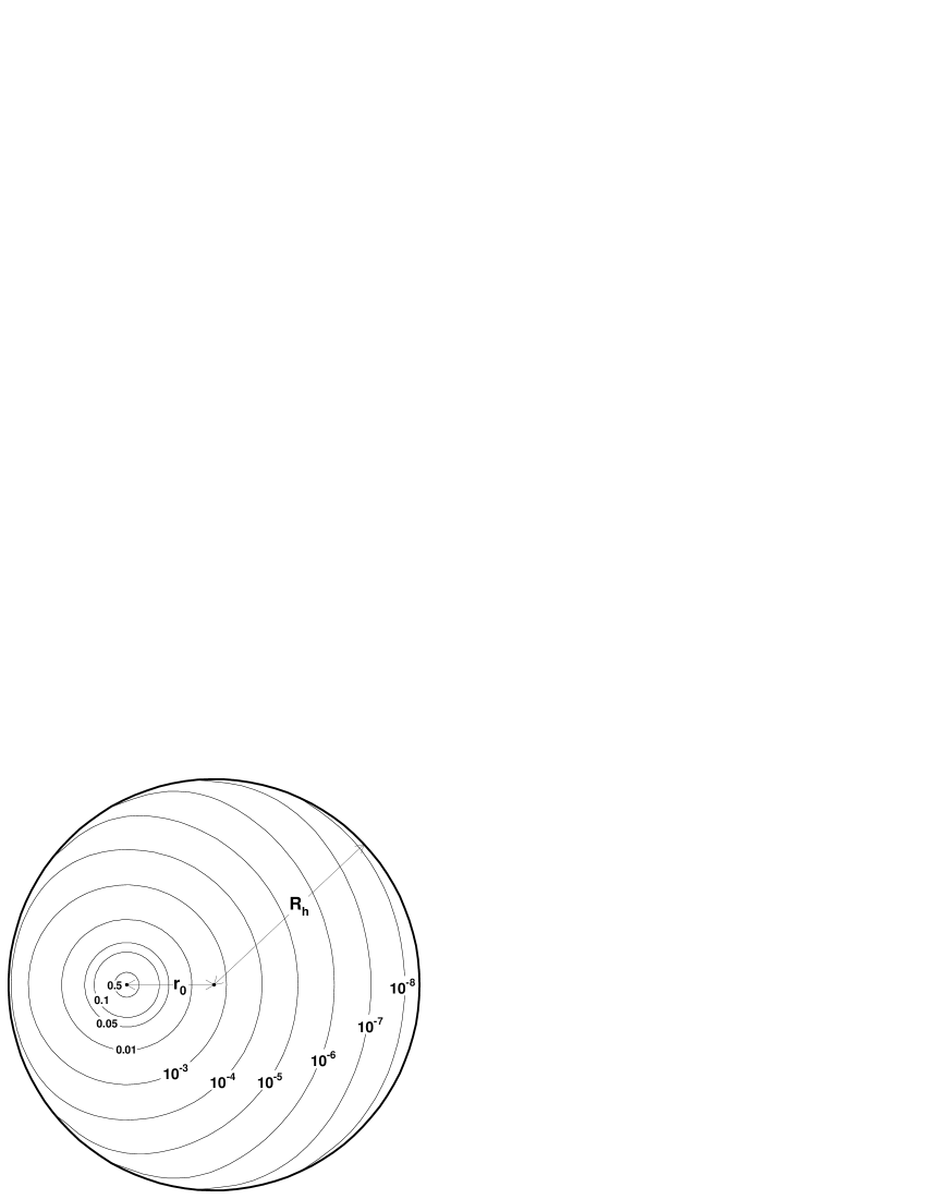
In Fig. 1 we plot $C_{\rm prop}^{cl}$ as a function of the distance $L$, choosing T=1 GeV and the set of canonical parameters for propagation model introduced in Paper I (diffusion zone height $h_{h}=3\,\rm{kpc}$, constant term in the diffusion coefficient $D^{0}=6\cdot 10^{27}\,\rm{cm}^{2}\rm{s}^{-1}$ and rigidity scale in the diffusion coefficient $R_{0}=3\,\rm{GV}$). The function we have drawn was computed fixing $z_{cl}$ and moving away from our position in the Galaxy in the direction of the galactic centre. As can be seen, we find at large distances a very accurate exponential scaling, while a sharp cusp appears below a distance of few kiloparsecs: the intuition that if the source happens to be close to us it gives a large contribution is confirmed. To show how accurate the assumption is that $C_{\rm prop}^{cl}$ is essentially just a function of $L$, we plot in Fig. 2 its isolevel curves in the plane $z_{cl}=1$ kpc. We have chosen to normalize $C_{\rm prop}^{cl}$ to 1 at 1 kpc above our position in the Galaxy. The isolevel curves are basically circumferences, which are just slightly deformed by our choice of fixing the antiproton number density to be zero at the border of the diffusion zone in the radial direction, i.e. $r=20$ kpc (thick solid line in the figure).

Figure 2: Isolevel curves for $C_{\rm prop}^{cl}$ in the plane $z_{cl}=1$ kpc. $C_{\rm prop}^{cl}$ has been normalized to 1 at 1 kpc above our position in the Galaxy. $r_{0}$ is our galactocentric distance.

We will not examine here the dependence of $C_{\rm prop}^{cl}$, and hence of the flux, on the parameters which define the propagation model: the results are analogous to what it was derived for $C_{\rm prop}$ in the smooth halo case. We just mention that introducing a galactic wind fixes a preferred direction of propagation and breaks therefore the scaling with distance.

As an example we consider the contribution to the antiproton flux given by a clump of neutralino dark matter defined by the same choice of parameters as in Bengtsson et al. (1990), where clumpiness was introduced in connection with the neutralino induced $\gamma$-ray signal with continuum energy spectrum. We fix hence $M_{cl}\sim 10^{8}M_{\odot}$ and $\delta\sim 10^{3}$; the prefactor $M_{cl}\delta$ is then about $1.3\cdot 10^{4}\rho_{0}\,\rm{kpc}^{3}$, where we assumed as local halo density $\rho_{0}=0.3\,\rm{GeV}\,\rm{cm}^{-3}$. Comparing the coefficient $C_{\rm prop}^{cl}$ with the analogous quantity in a smooth halo scenario (with the same choice of propagation model parameters $C_{\rm prop}(T=1\,\rm{GeV})\sim 10^{25}\,\rm{cm}\,\rm{sr}^{-1}$) we find that the antiproton flux from this single dark matter clump can be at the level (or much higher) than the sum of the contributions from the whole dark matter halo if this source is within about 4.5 kpc.

We might also consider an opposite approach. It is well established that a dark mass of at least $2\cdot 10^{6}M_{\odot}$ is concentrated within 0.015 pc at the galactic centre (Eckart & Genzel 1996), forming probably a massive black hole, possibly the astrophysical object which is called Sgr A^∗. Such accretion of matter might be associated to a region where the density of neutralino dark matter is enhanced as well. In an extreme scenario (Berezinsky et al. 1992) the potential well of a very steep dark matter halo profile ($\sim 1/r^{1.8}$) is the seed for the formation of the black hole itself. It is also intriguing that an excess in the high energy $\gamma$-ray flux from the galactic centre region, which has been found from the analysis of EGRET data (Mayer-Hasselwander et al. 1998), can be explained in terms of neutralino annihilations if an appropriate enhancement of the neutralino density is present there (Ullio 1999). Regardless of its possible origin, we can estimate how large the accretion of neutralinos at the galactic centre should be to give a measurable primary antiproton flux. Assuming that the galactocentric distance is 8.5 kpc, we find that the flux induced by a source at the galactic centre is proportional to $C_{\rm prop}^{cl}(8.5\,\rm{kpc})\sim 4.5\cdot 10^{19}\,\rm{cm}\,\rm{sr}^{-1}\,\rm{kpc}^{-3}$ (at T=1 GeV ). If we require for instance that its contribution should be at least one half of the total flux in a smooth halo scenario, we find that $M_{cl}\delta$ should be at least of the order of $10^{12}M_{\odot}$.

2.3 Collective effects of clumpiness

There is the possibility that a large fraction of the dark matter mass is in clumps, in the extreme case all of it. To avoid violating dynamical constraints, clumps should be light, with masses probably less than $M_{cl}\sim 10^{4}-10^{6}M_{\odot}$. If one could deal with a model that gives some accurate prediction for the masses of clumps and their distribution in the Galaxy, it would be possible to exploit the approach of the previous paragraph and estimate the antiproton flux by adding the contributions from individual sources. As very little is known about the inherently non linear problem of generating dark matter clumps, it seems more reasonable to follow a probabilistic approach.

Let $f$ be the fraction of dark matter in clumps and $N_{cl}$ the total number of clumps, all roughly of about the same mass and overdensity. We can define a probability density distribution of the clumps in the Galaxy which in the limit of large $f$, to fulfill dynamical constraints, has to follow the mass distribution in the halo. In a Cartesian coordinate system with origin at the galactic centre, the probability to find a given clump in the volume element $d^{\,3}x$ at position $\@vec{x}$ is:

$$p_{cl}(\@vec{x})\,d^{\,3}x=\frac{1}{M_{h}}\;\rho(\@vec{x})\,d^{\,3}x\;.$$ (5)

We introduced here $M_{h}$, the total mass of the halo, so that $p_{cl}$ has the correct normalization $\int p_{cl}(\@vec{x})d^{\,3}x=1$.

The antiproton source function in the volume element $d^{\,3}x$ at the galactic position $\@vec{x}$ is then:

$$Q_{\bar{p}}^{\chi\,\prime}(T,\@vec{x}\,)\,d^{\,3}x=(\sigma_{\rm ann}v)\frac{1}{{m_{\chi}}^{2}}\sum_{F}\frac{dN^{F}}{dT}B^{F}\cdot$$ (6)

$$\cdot N_{cl}\,p_{cl}(\@vec{x})\int d^{\,3}r_{cl}\,\left(\rho_{cl}(\@vec{r}_{cl})\right)^{2}\,d^{\,3}x$$

$$=f\,\delta\;\frac{\rho_{0}\;\rho(\@vec{x})}{{m_{\chi}}^{2}}(\sigma_{\rm ann}v)\sum_{F}\frac{dN^{F}}{dT}B^{F}\,d^{\,3}x\;,$$

while the antiproton flux is:

$$\Phi_{\bar{p}}^{\prime}(r_{0},T)=(\sigma_{\rm ann}v)\sum_{F}\frac{dN^{F}}{dT}B^{F}f\,\delta\;\frac{{\rho_{0}}^{2}}{{m_{\tilde{\chi}}}^{2}}\cdot$$ (7)

$$\cdot\,\int d^{\,3}x\,\frac{\rho(\@vec{x})}{\rho_{0}}C_{\rm prop}^{cl}(T,\@vec{x})$$

$$\equiv(\sigma_{\rm ann}v)\sum_{F}\frac{dN^{F}}{dT}B^{F}f\,\delta\;\frac{{\rho_{0}}^{2}}{{m_{\tilde{\chi}}}^{2}}C_{\rm prop}^{\prime}(T)\;.$$

In the equation above, $C_{\rm prop}^{\prime}(T)$ may actually be computed in the same way as the corresponding coefficient for a smooth halo $C_{\rm prop}(T)$, just by replacing in the former $(\rho(\@vec{x})/\rho_{0})^{2}$ with $\rho(\@vec{x})/\rho_{0}$. The two coefficients have similar behaviours; for our canonical diffusion parameters and an isothermal sphere as dark matter halo profile, $C_{\rm prop}^{\prime}\sim 0.75\cdot C_{\rm prop}$ for most of the kinetic energies of interest in our problem. The antiproton flux in the many small clump scenario can then be obtained by scaling the result in the smooth halo case by roughly $0.75\cdot f\,\delta$. There is quite a large freedom in the choice of $f\,\delta$, however one has to worry about not violating existing experimental bounds (Bergström et al. 1999a). In all the results in the next Section we have been careful to check that the models we propose do not induce an overproduction of both diffuse $\gamma$-rays and of cosmic positrons.

3 Signatures in the high energy antiproton spectrum

We have provided two schemes in which the antiproton flux can be sensibly enhanced with respect to the results in the smooth halo scenario. We propose here three cases in which the signal from neutralino dark matter annihilations in a clumpy halo can distort the high energy cosmic ray flux, giving a very clear signature of the presence of an exotic component.

Two experiments have measured the antiproton flux above a kinetic energy of few GeV (Golden et al. 1979; Hof et al. 1996) and their data are in contradiction with each other. A new set of experiments, the Caprice experiment (Boezio et al. 1997) and the space-based Ams (Ahlen et al. 1994) and Pamela (Adriani et al. 1995), should give much more abundant data in the near future. We will check that our predictions are consistent with the data in the low energy regime (below 3 GeV) from the Bess 97 (Orito 1998) and Bess 95 (Matsunaga et al. 1998) flights, which have given a first hint on the actual shape of the antiproton spectrum. The prediction for the background for our canonical set of parameters actually provides a very good fit of the data (see Paper I; our background prediction has been confirmed by Bieber et al. (1999) and is consistent in the high energy region with most the previous estimates in the literature). In the first two cases below we allow a little room for a neutralino-induced component by lowering the normalization of the primary proton flux by 1 $\sigma$.

For simplicity we will focus on the many small clumps scenario and quote in each case the value of the parameter $f\delta$ we are considering. The sample of supersymmetric models on which this analysis is based is the same as in Paper I. As in the smooth halo case we restrict to those MSSMs for which the neutralino has a cosmologically interesting relic density, e.g. $0.025<\Omega_{\chi}h^{2}<1$.

To compare with Bess data we have to take into account solar modulation. We relate the flux measured at the top of the atmosphere to the interstellar flux applying the force-field approximation by Gleeson & Axford (1967) with solar modulation parameter $\phi_{F}\sim 500$ MV (value suggested in the analysis of the Bess collaboration).

3.1 Broadening of the maximum in antiproton flux

Figure 3: Distorsion on the secondary antiproton flux (line $b$) induced by a signal from a heavy Higgsino-like neutralino.

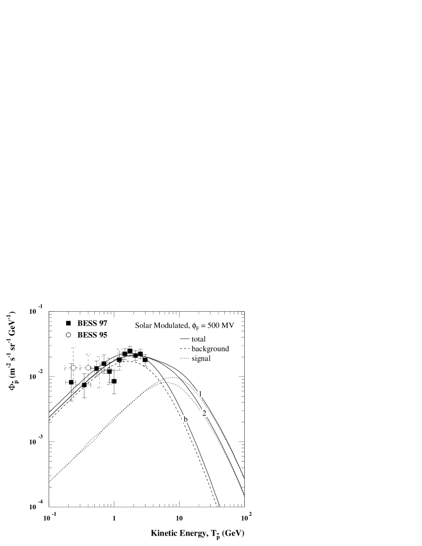
The prediction for the background secondary flux has a well defined maximum at about 2 GeV. We check if it is possible to introduce a distorsion in the spectrum by adding a component which widens the shape of the maximum. We will further require that this is not just some local distorsion which might be mimicked by introducing for instance reacceleration effects (Simon & Heinbach 1996). In our extreme case we impose that the antiproton flux from neutralino annihilations must exceed the estimate for the background by at least one order of magnitude at very high energies, say about 50 GeV. To obtain a wider maximum one has to add a neutralino signal rather sharply peaked at an energy higher than the maximum in the background; its spectrum should then decrease rapidly at low energies. The effect we are searching for might be produced by high mass neutralinos with negligible branching ratio into $b\bar{b}$ or $t\bar{t}$, which is the case e.g. for a very pure heavy Higgsino-like neutralino. In Fig. 3 we show two examples compared to our standard background estimate (solid line denoted with the letter $b$). Model 1 is a 964 GeV Higgsino ($Z_{g}=0.0027$) with flux rescaled by $f\,\delta=4180$; it is the model in our MSSM sample which gives the highest possible flux at 50 GeV compatibly with the background normalization we have chosen (dashed line in the figure) and with the requirement that added to the former it should give a good fit of the Bess data. Model 2 is instead the case in this class of examples which is associated with the lowest rescaling, $f\,\delta=1180$; it is at the same time the model with the smallest mass, an Higgsino-like neutralino ($Z_{g}=10^{-6}$) with $m_{\chi}=777$ GeV. A further reduction in the background or a less pronounced overproduction of antiprotons at high energies, allow lower values of both $m_{\chi}$ and $f\,\delta$.

Figure 4: Distorsion on the secondary antiproton flux (line $b$) induced by a neutralino signal with flat spectrum.

3.2 Break in the energy spectrum

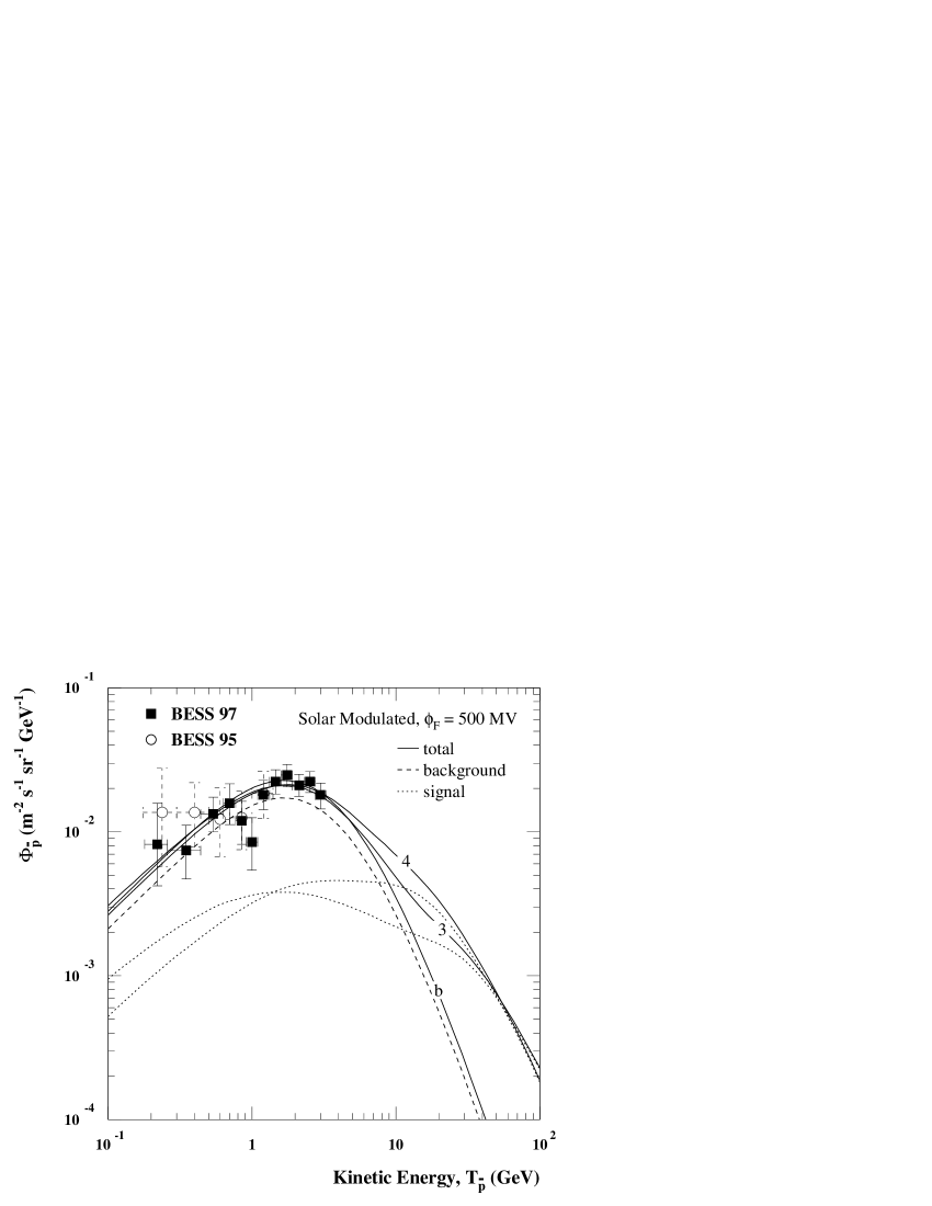
We focus in this case on rather flat neutralino-induced spectra. If one adds such a component to the background, the peak and the low energy tail in the antiproton flux are not sensibly affected, but a severe break may occur in the high energy region. A flat signal spectrum is generated overlapping a low contribution from a quark annihilation channel to a gauge boson contribution at higher energies. In Fig. 4 model 3 is the case in our MSSM sample which produces the flattest spectrum and therefore may induce the most severe break. It is a very heavy neutralino, $m_{\chi}=2730$ GeV, and the rescaling needed in this case may be uncomfortably high, $f\,\delta\sim 10^{5}$ (but still it does not violate any experimental constraint from other cosmic ray measurements). The second example, model 4, has a mass of 1400 GeV and $f\,\delta=7200$. Clearly these are extreme cases: in this category we may include a large fraction of models in our sample, which with a very mild rescaling give a distorsion of the flux at the highest energies. The chance of detecting less severe breaks in the energy spectrum clearly depends on how accurately the antiproton flux is measured.

3.3 Finite antiproton lifetime

Figure 5: Estimate of possible fluxes in case of finite antiproton lifetime $\tau_{\bar{p}}$, as compared with the standard background case when $\tau_{\bar{p}}=\infty$. The total flux is the sum of a neutralino induced component (not shown) and the secondary component (dashed lines) which, as plotted in the 3 examples, can be much suppressed compared to line $b$.

In exotic scenarios, the antiproton may have a finite lifetime $\tau_{\bar{p}}$. In the cosmic ray context this is an interesting ingredient in case $\tau_{\bar{p}}$ is lower than the characteristic escape time of antiprotons from the Galaxy. The escape time is determined by the parameters which define the propagation model; in our case it is about 10 Myr. This value is clearly much lower than the bound one can infer in CPT conserving theories from the experimental limit on the proton lifetime ($\tau_{\bar{p}}=\tau_{p}>10^{31}$ yr, see Caso et al. (1998)). On the other hand it is much larger than the most stringent direct experimental bound ($\tau_{\bar{p}}>0.05$ Myr from the $\bar{p}\rightarrow\mu^{-}\gamma$ decay mode, see Hu et al. (1998)).

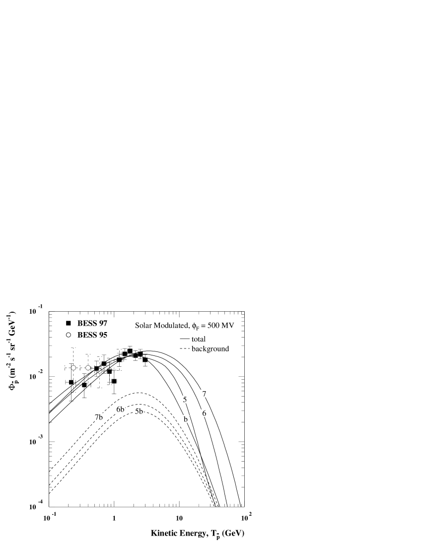
Geer & Kennedy (1998) have recently claimed that from cosmic ray measurement it is possible to infer a limit of $\tau_{\bar{p}}>0.8$ Myr (90% C.L.). In their analysis the secondary component only is included. Adding a neutralino signal obviously may change this result. Actually we show here that in a clumpy scenario, even in case of a finite antiproton lifetime, we can produce models which give at the same time a very good fit of the existing Bess data and whose spectral features are peculiar enough to be distinguished from the standard background once measurements at higher energies will be available. In Fig. 5 we compare three such models with the case of standard background and infinite $\tau_{\bar{p}}$. Model 5 is a 51 GeV gaugino-like neutralino whose antiproton flux has been scaled by $f\,\delta=49$ and for $\tau_{\bar{p}}=0.82$ Myr. Also shown in the figure is the reduction in the background flux induced by considering $\tau_{\bar{p}}=0.82$ Myr (dashed line labelled by $5b$). Model 7 is the heaviest model for which the predicted flux is still in excellent agreement with existing data (90% C.L. fit for $m_{\chi}=477$ GeV, $f\,\delta=1.2\cdot 10^{4}$ and $\tau_{\bar{p}}=2.92$ Myr), while model 6 is some intermediate case ($m_{\chi}=188$ GeV, $f\,\delta=78$ and $\tau_{\bar{p}}=1.32$ Myr). The trend is that for heavier neutralinos there is a larger overproduction of antiprotons in the high energy range.

Applying the largest possible rescalings consistent with $\gamma$-ray measurements we find that a 56 GeV neutralino model gives a flux which is consistent with Bess data at 90% C.L. in case the antiproton lifetime is as low as $\tau_{\bar{p}}=0.15$ Myr. The bound of Geer & Kennedy (1998) is clearly violated. Notice that we are comparing with a more aboundant data set than in that reference (Bess 97 data were not included there) and that we used our standard values for the parameters which define the diffusion model and solar modulation. If uncertainties were included the lower bound we would get with this method would probably be very close to the most stringent direct experimental bound $\tau_{\bar{p}}>0.05$ Myr or lower.

4 Conclusion

To conclude, we have shown that there is a chance of detecting neutralino dark matter in upcoming measurements of the cosmic antiproton flux at high energies. The signatures we propose here are alternative to the signature of an exotic component at low kinetic energies, which seems not to be required by present data. We have also discussed the possibility that antiprotons have a finite lifetime and shown that the limit on $\tau_{\bar{p}}$ which is possible to set on the basis of cosmic ray measurements is comparable to those in direct experiments.

Acknowlegements

I am grateful to Lars Bergström and Joakim Edsjö for many useful discussions. I thank Paolo Gondolo for collaboration on the numerical supersymmetry calculations.

References

- (1) Adriani, O., et al., 1995, in Proc. of 24th ICRC, Rome, 3, 591
- (2) Ahlen, S., et al., 1994, Nucl. Instrum. Meth. A350, 351
- (3) Bengtsson, H.-U., Salati, P., Silk, J., 1990, Nucl. Phys. B346, 129
- (4) Berezinsky, V.S., Gurevich, A.V., Zybin, K.P., 1992, Phys. Lett. B294, 221
- (5) Bergström, L., Edsjö, J., Gondolo, P., Ullio, P., 1999a, Phys. Rev. D59, 043506
- (6) Bergström, L., Edsjö, Ullio, P., 1999b, ApJ submitted (astro-ph/9902012)
- (7) Bergström, L., Gondolo, P., 1996, Astrop. Phys. 5, 263
- (8) Bieber, J.W., et al., 1999, submitted (astro-ph/9903163)
- (9) Bottino, A., Donato, F., Fornengo, N., Salati, P., 1998, Phys. Rev. D58, 123503
- (10) Boezio, M., et al., 1997, ApJ 487, 415
- (11) Buffington, A., et al., 1981, ApJ 248, 1179
- (12) Caso, C., et al., (Particle Data Group), 1998, European Phys. J. C3, 1
- (13) Eckart, A., Genzel, R., 1996, Nat 383, 415
- (14) Geer, S.H., Kennedy, D.C., 1998 submitted (astro-ph/9812025)
- (15) Gleeson, L.J., Axford, W.I., 1967, ApJ 149, L115
- (16) Golden, R.L., et al., 1979, Phys. Rev. Lett. 43, 1196
- (17) Hu. M., et al., (APEX Collab), 1998, Phys. Rev. D58, 111101
- (18) Kolb, E.W., Tkachev, I.I., 1994, Phys. Rev. D50, 769
- (19) Matsunaga, H., et al., 1998, Phys. Rev. Lett. 81, 4052
- (20) Mayer-Hasselwander, H.A., et al., 1998, A&A 335, 161
- (21) Orito, S., 1998, Talk given at The 29th International Conference on High-Energy Physics, Vancouver, 1998
- (22) Silk, J., Srednicki, M., 1984, Phys. Rev. Lett. 50, 624
- (23) Silk, J., Stebbins, A., 1993, ApJ 411, 439
- (24) Silk, J., Szalay, A.S., 1987, ApJ 323, L107
- (25) Simon, M., Heinbach, U., 1996, ApJ 456, 519
- (26) Sjöstrand, T., 1994, Comput. Phys. Commun. 82, 74
- (27) Stecker, F.W., Rudaz, S., Walsh, T.F., 1985, Phys. Rev. Lett. 55, 2622
- (28) Ullio, P., 1999, Indirect Detection of Neutralino Dark Matter, (Stockholm University Ph.D. thesis), to be published