Why Cosmologists Believe the Universe is Accelerating

Abstract

Theoretical cosmologists were quick to be convinced by the evidence presented in 1998 for the accelerating Universe. I explain how this remarkable discovery was the missing piece in the grand cosmological puzzle. When found, it fit perfectly. For cosmologists, this added extra weight to the strong evidence of the SN Ia measurements themselves, making the result all the more believable.

1 Introduction

If theoretical cosmologists are the flyboys of astrophysics, they were flying on fumes in the 1990s. Since the early 1980s inflation and cold dark matter (CDM) have been the dominant theoretical ideas in cosmology. However, a key prediction of inflation, a flat Universe (i.e., $\Omega_{0}\equiv\rho_{\rm total}/\rho_{\rm crit}=1$), was beginning to look untenable. By the late 1990s it was becoming increasingly clear that matter only accounted for 30% to 40% of the critical density (see e.g., Turner, 1999). Further, the $\Omega_{M}=1$, COBE-normalized CDM model was not a very good fit to the data without some embellishment (15% or so of the dark matter in neutrinos, significant deviation from from scale invariance – called tilt – or a very low value for the Hubble constant; see e.g., Dodelson et al., 1996).

Because of this and their strong belief in inflation, a number of inflationists (see e.g., Turner, Steigman & Krauss, 1984 and Peebles, 1984) were led to consider seriously the possibility that the missing 60% or so of the critical density exists in the form of vacuum energy (cosmological constant) or something even more interesting with similar properties (see Sec. 3 below). Since determinations of the matter density take advantage of its enhanced gravity when it clumps (in galaxies, clusters or superclusters), vacuum energy, which is by definition spatially smooth, would not have shown up in the matter inventory.

Not only did a cosmological constant solve the “$\Omega$ problem,” but $\Lambda$CDM, the flat CDM model with $\Omega_{M}\sim 0.4$ and $\Omega_{\Lambda}\sim 0.6$, became the best fit universe model (Turner, 1991 and 1997b; Krauss & Turner, 1995; Ostriker & Steinhardt, 1995; Liddle et al., 1996). In June 1996, at the Critical Dialogues in Cosmology Meeting at Princeton University, the only strike recorded against $\Lambda$CDM was the early SN Ia results of Perlmutter’s group (Perlmutter et al., 1997) which excluded $\Omega_{\Lambda}>0.5$ with 95% confidence.

The first indirect experimental hint for something like a cosmological constant came in 1997. Measurements of the anisotropy of the cosmic background radiation (CBR) began to show evidence for the signature of a flat Universe, a peak in the multipole power spectrum at $l=200$. Unless the estimates of the matter density were wildly wrong, this was evidence for a smooth, dark energy component. A universe with $\Omega_{\Lambda}\sim 0.6$ has a smoking gun signature: it is speeding up rather than slowing down. In 1998 came the SN Ia evidence that our Universe is speeding up; for some cosmologists this was a great surprise. For many theoretical cosmologists this was the missing piece of the grand puzzle and the confirmation of a prediction.

2 The theoretical case for accelerated expansion

The case for accelerated expansion that existed in January 1998 had three legs: growing evidence that $\Omega_{M}\sim 0.4$ and not 1; the inflationary prediction of a flat Universe and hints from CBR anisotropy that this was indeed true; and the failure of simple $\Omega_{M}=1$ CDM model and the success of $\Lambda$CDM. The tension between measurements of the Hubble constant and age determinations for the oldest stars was also suggestive, though because of the uncertainties, not as compelling. Taken together, they foreshadowed the presence of a cosmological constant (or something similar) and the discovery of accelerated expansion.

To be more precise, Sandage’s deceleration parameter is given by

$$q_{0}\equiv{(\ddot{R}/R)_{0}\over H_{0}^{2}}={1\over 2}\Omega_{0}+{3\over 2}\sum_{i}\Omega_{i}w_{i}\,,$$ (2.1)

where the pressure of component $i$, $p_{i}\equiv w_{i}\rho_{i}$; e.g., for baryons $w_{i}=0$, for radiation $w_{i}=1/3$, and for vacuum energy $w_{X}=-1$. For $\Omega_{0}=1$, $\Omega_{M}=0.4$ and $w_{X}<-{5\over 9}$, the deceleration parameter is negative. The kind of dark component needed to pull cosmology together implies accelerated expansion.

2.1 Matter/energy inventory: $\Omega_{0}=1\pm 0.2$, $\Omega_{M}=0.4\pm 0.1$

There is a growing consensus that the anisotropy of the CBR offers the best means of determining the curvature of the Universe and thereby $\Omega_{0}$. This is because the method is intrinsically geometric – a standard ruler on the last-scattering surface – and involves straightforward physics at a simpler time (see e.g., Kamionkowski et al., 1994). It works like this.

At last scattering baryonic matter (ions and electrons) was still tightly coupled to photons; as the baryons fell into the dark-matter potential wells the pressure of photons acted as a restoring force, and gravity-driven acoustic oscillations resulted. These oscillations can be decomposed into their Fourier modes; Fourier modes with $k\sim lH_{0}/2$ determine the multipole amplitudes $a_{lm}$ of CBR anisotropy. Last scattering occurs over a short time, making the CBR is a snapshot of the Universe at $t_{\rm ls}\sim 300,000\,$yrs. Each mode is “seen” in a well defined phase of its oscillation. (For the density perturbations predicted by inflation, all modes the have same initial phase because all are growing-mode perturbations.) Modes caught at maximum compression or rarefaction lead to the largest temperature anisotropy; this results in a series of acoustic peaks beginning at $l\sim 200$ (see Fig. 1). The wavelength of the lowest frequency acoustic mode that has reached maximum compression, $\lambda_{\rm max}\sim v_{s}t_{\rm ls}$, is the standard ruler on the last-scattering surface. Both $\lambda_{\rm max}$ and the distance to the last-scattering surface depend upon $\Omega_{0}$, and the position of the first peak $l\simeq 200/\sqrt{\Omega_{0}}$. This relationship is insensitive to the composition of matter and energy in the Universe.

CBR anisotropy measurements, shown in Fig. 1, now cover three orders of magnitude in multipole and are from more than twenty experiments. COBE is the most precise and covers multipoles $l=2-20$; the other measurements come from balloon-borne, Antarctica-based and ground-based experiments using both low-frequency ($f<100\,$GHz) HEMT receivers and high-frequency ($f>100\,$GHz) bolometers. Taken together, all the measurements are beginning to define the position of the first acoustic peak, at a value that is consistent with a flat Universe. Various analyses of the extant data have been carried out, indicating $\Omega_{0}\sim 1\pm 0.2$ (see e.g., Lineweaver, 1998). It is certainly too early to draw definite conclusions or put too much weigh in the error estimate. However, a strong case is developing for a flat Universe and more data is on the way (Python V, Viper, MAT, Maxima, Boomerang, CBI, DASI, and others). Ultimately, the issue will be settled by NASA’s MAP (launch late 2000) and ESA’s Planck (launch 2007) satellites which will map the entire CBR sky with 30 times the resolution of COBE (around $0.1^{\circ}$) (see Page and Wilkinson, 1999).

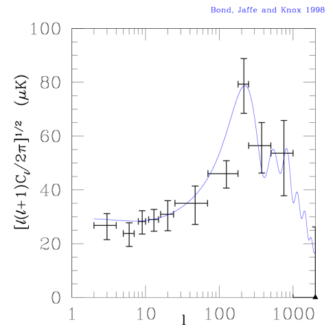
Figure 1: Current CBR anisotropy data, averaged and binned to reduce error bars and visual confusion. The theoretical curve is for the $\Lambda$CDM model with $H_{0}=65\,{\rm km\,s^{-1}\,Mpc^{-1}}$ and $\Omega_{M}=0.4$; note the goodness of fit (Figure courtesy of L. Knox).

Since the pioneering work of Fritz Zwicky and Vera Rubin, it has been known that there is far too little material in the form of stars (and related material) to hold galaxies and clusters together, and thus, that most of the matter in the Universe is dark (see e.g. Trimble, 1987). Weighing the dark matter has been the challenge. At present, I believe that clusters provide the most reliable means of estimating the total matter density.

Rich clusters are relatively rare objects – only about 1 in 10 galaxies is found in a rich cluster – which formed from density perturbations of (comoving) size around 10 Mpc. However, because they gather together material from such a large region of space, they can provide a “fair sample” of matter in the Universe. Using clusters as such, the precise BBN baryon density can be used to infer the total matter density (White et al., 1993). (Baryons and dark matter need not be well mixed for this method to work provided that the baryonic and total mass are determined over a large enough portion of the cluster.)

Most of the baryons in clusters reside in the hot, x-ray emitting intracluster gas and not in the galaxies themselves, and so the problem essentially reduces to determining the gas-to-total mass ratio. The gas mass can be determined by two methods: 1) measuring the x-ray flux from the intracluster gas and 2) mapping the Sunyaev - Zel’dovich CBR distortion caused by CBR photons scattering off hot electrons in the intracluster gas. The total cluster mass can be determined three independent ways: 1) using the motions of clusters galaxies and the virial theorem; 2) assuming that the gas is in hydrostatic equilibrium and using it to infer the underlying mass distribution; and 3) mapping the cluster mass directly by gravitational lensing (Tyson, 1999). Within their uncertainties, and where comparisons can be made, the three methods for determining the total mass agree (see e.g., Tyson, 1999); likewise, the two methods for determining the gas mass are consistent.

Mohr et al. (1998) have compiled the gas to total mass ratios determined from x-ray measurements for a sample of 45 clusters; they find $f_{\rm gas}=(0.075\pm 0.002)h^{-3/2}$ (see Fig. 2). Carlstrom (1999), using his S-Z gas measurements and x-ray measurements for the total mass for 27 clusters, finds $f_{\rm gas}=(0.06\pm 0.006)h^{-1}$. (The agreement of these two numbers means that clumping of the gas, which could lead to an overestimate of the gas fraction based upon the x-ray flux, is not a problem.) Invoking the “fair-sample assumption,” the mean matter density in the Universe can be inferred:

$$\Omega_{M}=\Omega_{B}/f_{\rm gas} = (0.3\pm 0.05)h^{-1/2}\ ({\rm Xray})$$ (2.2)

$$= (0.25\pm 0.04)h^{-1}\ ({\rm S-Z})$$

$$= 0.4\pm 0.1\ ({\rm my\ summary})\,.$$

I believe this to be the most reliable and precise determination of the matter density. It involves few assumptions, most of which have now been tested. For example, the agreement of S-Z and x-ray gas masses implies that gas clumping is not significant; the agreement of x-ray and lensing estimates for the total mass implies that hydrostatic equilibrium is a good assumption; the gas fraction does not vary significantly with cluster mass.

Figure 2: Cluster gas fraction as a function of cluster gas temperature for a sample of 45 galaxy clusters (Mohr et al., 1998). While there is some indication that the gas fraction decreases with temperature for $T<5\,$keV, perhaps because these lower-mass clusters lose some of their hot gas, the data indicate that the gas fraction reaches a plateau at high temperatures, $f_{\rm gas}=0.212\pm 0.006$ for $h=0.5$ (Figure courtesy of Joe Mohr).

2.2 Dark energy

The apparently contradictory results, $\Omega_{0}=1\pm 0.2$ and $\Omega_{M}=0.4\pm 0.1$, can be reconciled by the presence of a dark-energy component that is nearly smoothly distributed. The cosmological constant is the simplest possibility and it has $p_{X}=-\rho_{X}$. There are other possibilities for the smooth, dark energy. As I now discuss, other constraints imply that such a component must have very negative pressure ($w_{X}\mathrel{\mathchoice{\lower 3.6pt\vbox{\halign{$\mathsurround=0pt\displaystyle\hfil#\hfil$\cr<\crcr\sim\crcr}}}{\lower 3.6pt\vbox{\halign{$\mathsurround=0pt\textstyle\hfil#\hfil$\cr<\crcr\sim\crcr}}}{\lower 3.6pt\vbox{\halign{$\mathsurround=0pt\scriptstyle\hfil#\hfil$\cr<\crcr\sim\crcr}}}{\lower 3.6pt\vbox{\halign{$\mathsurround=0pt\scriptscriptstyle\hfil#\hfil$\cr<\crcr\sim\crcr}}}}-{1\over 2}$) leading to the prediction of accelerated expansion.

To begin, parameterize the bulk equation of state of this unknown component: $w\equiv p_{X}/\rho_{X}$ (Turner & White, 1997). This implies that its energy density evolves as $\rho_{X}\propto R^{-n}$ where $n=3(1+w)$. The development of the structure observed today from density perturbations of the size inferred from measurements of the anisotropy of the CBR requires that the Universe be matter dominated from the epoch of matter – radiation equality until very recently. Thus, to avoid interfering with structure formation, the dark-energy component must be less important in the past than it is today. This implies that $n$ must be less than $3$ or $w<0$; the more negative $w$ is, the faster this component gets out of the way (see Fig. 3). More careful consideration of the growth of structure implies that $w$ must be less than about $-{1\over 3}$ (Turner & White, 1997).

Next, consider the constraint provided by the age of the Universe and the Hubble constant. Their product, $H_{0}t_{0}$, depends the equation of state of the Universe; in particular, $H_{0}t_{0}$ increases with decreasing $w$ (see Fig. 4). To be definite, I will take $t_{0}=14\pm 1.5\,$Gyr and $H_{0}=65\pm 5\,{\rm km\,s^{-1}\,Mpc^{-1}}$ (see e.g., Chaboyer et al., 1998 and Freedman, 1999); this implies that $H_{0}t_{0}=0.93\pm 0.13$. Fig. 4 shows that $w<-{1\over 2}$ is preferred by age/Hubble constant considerations.

Figure 3: Evolution of the energy density in matter, radiation (heavy lines), and different possibilities for the dark-energy component ($w=-1,-{1\over 3},{1\over 3}$) vs. scale factor. The matter-dominated era begins when the scale factor was $\sim 10^{-4}$ of its present size (off the figure) and ends when the dark-energy component begins to dominate, which depends upon the value of $w$: the more negative $w$ is, the longer the matter-dominated era in which density perturbations can go into the large-scale structure seen today. These considerations require $w<-{1\over 3}$ (Turner & White, 1997).

Figure 4: $H_{0}t_{0}$ vs. the equation of state for the dark-energy component. As can be seen, an added benefit of a component with negative pressure is an older Universe for a given Hubble constant. The broken horizontal lines denote the $1\sigma$ range for $H_{0}=65\pm 5\,{\rm km\,s^{-1}\,Mpc^{-1}}$ and $t_{0}=14\pm 1.5\,$Gyr, and indicate that $w<-{1\over 2}$ is preferred.

To summarize, consistency between $\Omega_{M}\sim 0.4$ and $\Omega_{0}\sim 1$ along with other cosmological considerations implies the existence of a dark-energy component with bulk pressure more negative than about $-\rho_{X}/2$. The simplest example of such is vacuum energy (Einstein’s cosmological constant), for which $w=-1$. The smoking-gun signature of a smooth, dark-energy component is accelerated expansion since $q_{0}=0.5+1.5w_{X}\Omega_{X}\simeq 0.5+0.9w<0$ for $w<-{5\over 9}$.

2.3 $\Lambda$CDM

The cold dark matter scenario for structure formation is the most quantitative and most successful model ever proposed. Two of its key features are inspired by inflation: almost scale invariant, adiabatic density perturbations with Gaussian statistical properties and a critical density Universe. The third, nonbaryonic dark matter is a logical consequence of the inflationary prediction of a flat universe and the BBN-determination of the baryon density at 5% of the critical density.

There is a very large body of data that is consistent with it: the formation epoch of galaxies and distribution of galaxy masses, galaxy correlation function and its evolution, abundance of clusters and its evolution, large-scale structure, and on and on. In the early 1980s attention was focused on a “standard CDM model”: $\Omega_{0}=\Omega_{M}=1$, $\Omega_{B}=0.05$, $h=0.50$, and exactly scale invariant density perturbations (the cosmological equivalent of DOS 1.0). The detection of CBR anisotropy by COBE DMR in 1992 changed everything.

First and most importantly, the COBE DMR detection validated the gravitational instability picture for the growth of large-scale structure: The level of matter inhomogeneity implied at last scattering, after 14 billion years of gravitational amplification, was consistent with the structure seen in the Universe today. Second, the anisotropy, which was detected on the $10^{\circ}$ angular scale, permitted an accurate normalization of the CDM power spectrum. For “standard cold dark matter”, this meant that the level of inhomogeneity on all scales could be accurately predicted. It turned out to be about a factor of two too large on galactic scales. Not bad for an ab initio theory.

With the COBE detection came the realization that the quantity and quality of data that bear on CDM was increasing and that the theoretical predictions would have to match their precision. Almost overnight, CDM became a ten (or so) parameter theory. For astrophysicists, and especially cosmologists, this is daunting, as it may seem that a ten-parameter theory can be made to fit any set of observations. This is not the case when one has the quality and quantity of data that will soon be available.

In fact, the ten parameters of CDM + Inflation are an opportunity rather than a curse: Because the parameters depend upon the underlying inflationary model and fundamental aspects of the Universe, we have the very real possibility of learning much about the Universe and inflation. The ten parameters can be organized into two groups: cosmological and dark-matter (Dodelson et al., 1996).

Cosmological Parameters

1. $h$, the Hubble constant in units of $100\,{\rm km\,s^{-1}}\,{\rm Mpc}^{-1}$.

2. $\Omega_{B}h^{2}$, the baryon density. Primeval deuterium measurements and together with the theory of BBN imply: $\Omega_{B}h^{2}=0.02\pm 0.002$.

3. $n$, the power-law index of the scalar density perturbations. CBR measurements indicate $n=1.1\pm 0.2$; $n=1$ corresponds to scale-invariant density perturbations. Many inflationary models predict $n\simeq 0.95$; range of predictions runs from $0.7$ to $1.2$.

4. $dn/d\ln k$, “running” of the scalar index with comoving scale ($k=$ wavenumber). Inflationary models predict a value of ${\cal O}(\pm 10^{-3})$ or smaller.

5. $S$, the overall amplitude squared of density perturbations, quantified by their contribution to the variance of the CBR quadrupole anisotropy.

6. $T$, the overall amplitude squared of gravity waves, quantified by their contribution to the variance of the CBR quadrupole anisotropy. Note, the COBE normalization determines $T+S$ (see below).

7. $n_{T}$, the power-law index of the gravity wave spectrum. Scale-invariance corresponds to $n_{T}=0$; for inflation, $n_{T}$ is given by $-{1\over 7}{T\over S}$.

Dark-matter Parameters

1. $\Omega_{\nu}$, the fraction of critical density in neutrinos ($=\sum_{i}m_{\nu_{i}}/90h^{2}$). While the hot dark matter theory of structure formation is not viable, we now know that neutrinos contribute at least 0.3% of the critical density (Fukuda et al., 1998).

2. $\Omega_{X}$ and $w_{X}$, the fraction of critical density in a smooth dark-energy component and its equation of state. The simplest example is a cosmological constant ($w_{X}=-1$).

3. $g_{*}$, the quantity that counts the number of ultra-relativistic degrees of freedom. The standard cosmology/standard model of particle physics predicts $g_{*}=3.3626$. The amount of radiation controls when the Universe became matter dominated and thus affects the present spectrum of density inhomogeneity.

A useful way to organize the different CDM models is by their dark-matter content; within each CDM family, the cosmological parameters vary. One list of models is:

1. sCDM (for simple): Only CDM and baryons; no additional radiation ($g_{*}=3.36$). The original standard CDM is a member of this family ($h=0.50$, $n=1.00$, $\Omega_{B}=0.05$), but is now ruled out (see Fig. 5).

2. $\tau$CDM: This model has extra radiation, e.g., produced by the decay of an unstable massive tau neutrino (hence the name); here we take $g_{*}=7.45$.

3. $\nu$CDM (for neutrinos): This model has a dash of hot dark matter; here we take $\Omega_{\nu}=0.2$ (about 5 eV worth of neutrinos).

4. $\Lambda$CDM (for cosmological constant) or more generally xCDM: This model has a smooth dark-energy component; here, we take $\Omega_{X}=\Omega_{\Lambda}=0.6$.

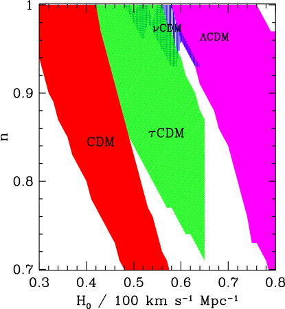
Figure 5: Summary of viable CDM models, based upon CBR anisotropy and determinations of the present power spectrum of inhomogeneity (Dodelson et al., 1996).

Figure 5 summarizes the viability of these different CDM models, based upon CBR measurements and current determinations of the present power spectrum of inhomogeneity (derived from redshift surveys). sCDM is only viable for low values of the Hubble constant (less than $55\,{\rm km\,s^{-1}}\,{\rm Mpc}^{-1}$) and/or significant tilt (deviation from scale invariance); the region of viability for $\tau$CDM is similar to sCDM, but shifted to larger values of the Hubble constant (as large as $65\,{\rm km\,s^{-1}}\,{\rm Mpc}^{-1}$). $\nu$CDM has an island of viability around $H_{0}\sim 60\,{\rm km\,s^{-1}}\,{\rm Mpc}^{-1}$ and $n\sim 0.95$. $\Lambda$CDM can tolerate the largest values of the Hubble constant. While the COBE DMR detection ruled out “standard CDM,” a host of attractive variants were still viable.

However, when other very relevant data are considered too – e.g., age of the Universe, determinations of the cluster baryon fraction, measurements of the Hubble constant, and limits to $\Omega_{\Lambda}$ – $\Lambda$CDM emerges as the hands-down-winner of “best-fit CDM model” (Krauss & Turner, 1995; Ostriker & Steinhardt, 1995; Liddle et al., 1996; Turner, 1997b). At the time of the Critical Dialogues in Cosmology meeting in 1996, the only strike against $\Lambda$CDM was the absence of evidence for its smoking gun signature, accelerated expansion.

Figure 6: Constraints used to determine the best-fit CDM model: PS = large-scale structure + CBR anisotropy; AGE = age of the Universe; CBF = cluster-baryon fraction; and $H_{0}$= Hubble constant measurements. The best-fit model, indicated by the darkest region, has $H_{0}\simeq 60-65\,{\rm km\,s^{-1}\,Mpc^{-1}}$ and $\Omega_{\Lambda}\simeq 0.55-0.65$. Evidence for its smoking-gun signature – accelerated expansion – was presented in 1998 (adapted from Krauss & Turner, 1995 and Turner, 1997).

2.4 Missing energy found!

In 1998 evidence for the accelerated expansion anticipated by theorists was presented in the form of the magnitude – redshift (Hubble) diagram for fifty-some type Ia supernovae (SNe Ia) out to redshifts of nearly 1. Two groups, the Supernova Cosmology Project (Perlmutter et al., 1998) and the High-z Supernova Search Team (Riess et al., 1998), working independently and using different methods of analysis, each found evidence for accelerated expansion. Perlmutter et al. (1998) summarize their results as a constraint to a cosmological constant (see Fig. 7),

$$\Omega_{\Lambda}={4\over 3}\Omega_{M}+{1\over 3}\pm{1\over 6}\,.$$ (2.3)

For $\Omega_{M}\sim 0.4\pm 0.1$, this implies $\Omega_{\Lambda}=0.85\pm 0.2$, or just what is needed to account for the missing energy! As I have tried to explain, cosmologists were quick than most to believe, as accelerated expansion was the missing piece of the puzzle found.

Recently, two other studies, one based upon the x-ray properties of rich clusters of galaxies (Mohr et al., 1999) and the other based upon the properties of double-lobe radio galaxies (Guerra et al., 1998), have reported evidence for a cosmological constant (or similar dark-energy component) that is consistent with the SN Ia results (i.e., $\Omega_{\Lambda}\sim 0.7$).

There is another test of an accelerating Universe whose results are more ambiguous. It is based upon the fact that the frequency of multiply lensed QSOs is expected to be significantly higher in an accelerating universe (Turner, 1990). Kochanek (1996) has used gravitational lensing of QSOs to place a 95% cl upper limit, $\Omega_{\Lambda}<0.66$; and Waga and Miceli (1998) have generalized it to a dark-energy component with negative pressure: $\Omega_{X}<1.3+0.55w$ (95% cl), both results for a flat Universe. On the other hand, Chiba and Yoshii (1998) claim evidence for a cosmological constant, $\Omega_{\Lambda}=0.7^{+0.1}_{-0.2}$, based upon the same data. From this I conclude: 1) Lensing excludes $\Omega_{\Lambda}$ larger than 0.8; 2) Because of the modeling uncertainties and lack of sensitivity for $\Omega_{\Lambda}<0.55$, lensing has little power in strictly constraining $\Lambda$ or a dark component; and 3) When larger objective surveys of gravitational-lensed QSOs are carried out (e.g., the Sloan Digital Sky Survey), there is the possibility of uncovering another smoking-gun for accelerated expansion.

2.5 Cosmic concordance

With the SN Ia results we have for the first time a complete and self-consistent accounting of mass and energy in the Universe. The consistency of the matter/energy accounting is illustrated in Fig. 7. Let me explain this exciting figure. The SN Ia results are sensitive to the acceleration (or deceleration) of the expansion and constrain the combination ${4\over 3}\Omega_{M}-\Omega_{\Lambda}$. (Note, $q_{0}={1\over 2}\Omega_{M}-\Omega_{\Lambda}$; ${4\over 3}\Omega_{M}-\Omega_{\Lambda}$ corresponds to the deceleration parameter at redshift $z\sim 0.4$, the median redshift of these samples). The (approximately) orthogonal combination, $\Omega_{0}=\Omega_{M}+\Omega_{\Lambda}$ is constrained by CBR anisotropy. Together, they define a concordance region around $\Omega_{0}\sim 1$, $\Omega_{M}\sim 1/3$, and $\Omega_{\Lambda}\sim 2/3$. The constraint to the matter density alone, $\Omega_{M}=0.4\pm 0.1$, provides a cross check, and it is consistent with these numbers. Further, these numbers point to $\Lambda$CDM (or something similar) as the cold dark matter model. Another body of observations already support this as the best fit model. Cosmic concordance indeed!

Figure 7: Two-$\sigma$ constraints to $\Omega_{M}$ and $\Omega_{\Lambda}$ from CBR anisotropy, SNe Ia, and measurements of clustered matter. Lines of constant $\Omega_{0}$ are diagonal, with a flat Universe shown by the broken line. The concordance region is shown in bold: $\Omega_{M}\sim 1/3$, $\Omega_{\Lambda}\sim 2/3$, and $\Omega_{0}\sim 1$. (Particle physicists who rotate the figure by $90^{\circ}$ will recognize the similarity to the convergence of the gauge coupling constants.)

3 What is the dark energy?

I have often used the term exotic to refer to particle dark matter. That term will now have to be reserved for the dark energy that is causing the accelerated expansion of the Universe – by any standard, it is more exotic and more poorly understood. Here is what we do know: it contributes about 60% of the critical density; it has pressure more negative than about $-\rho/2$; and it does not clump (otherwise it would have contributed to estimates of the mass density). The simplest possibility is the energy associated with the virtual particles that populate the quantum vacuum; in this case $p=-\rho$ and the dark energy is absolutely spatially and temporally uniform.

This “simple” interpretation has its difficulties. Einstein “invented” the cosmological constant to make a static model of the Universe and then he discarded it; we now know that the concept is not optional. The cosmological constant corresponds to the energy associated with the vacuum. However, there is no sensible calculation of that energy (see e.g., Zel’dovich, 1967; Bludman and Ruderman, 1977; and Weinberg, 1989), with estimates ranging from $10^{122}$ to $10^{55}$ times the critical density. Some particle physicists believe that when the problem is understood, the answer will be zero. Spurred in part by the possibility that cosmologists may have actually weighed the vacuum (!), particle theorists are taking a fresh look at the problem (see e.g., Harvey, 1998; Sundrum, 1997). Sundrum’s proposal, that the gravitational energy of the vacuum is close to the present critical density because the graviton is a composite particle with size of order 1 cm, is indicative of the profound consequences that a cosmological constant has for fundamental physics.

Because of the theoretical problems mentioned above, as well as the checkered history of the cosmological constant, theorists have explored other possibilities for a smooth, component to the dark energy (see e.g., Turner & White, 1997). Wilczek and I pointed out that even if the energy of the true vacuum is zero, as the Universe as cooled and went through a series of phase transitions, it could have become hung up in a metastable vacuum with nonzero vacuum energy (Turner & Wilczek, 1982). In the context of string theory, where there are a very large number of energy-equivalent vacua, this becomes a more interesting possibility: perhaps the degeneracy of vacuum states is broken by very small effects, so small that we were not steered into the lowest energy vacuum during the earliest moments.

Vilenkin (1984) has suggested a tangled network of very light cosmic strings (also see, Spergel & Pen, 1997) produced at the electroweak phase transition; networks of other frustrated defects (e.g., walls) are also possible. In general, the bulk equation-of-state of frustrated defects is characterized by $w=-N/3$ where $N$ is the dimension of the defect ($N=1$ for strings, $=2$ for walls, etc.). The SN Ia data almost exclude strings, but still allow walls.

An alternative that has received a lot of attention is the idea of a “decaying cosmological constant”, a termed coined by the Soviet cosmologist Matvei Petrovich Bronstein in 1933 (Bronstein, 1933). (Bronstein was executed on Stalin’s orders in 1938, presumably for reasons not directly related to the cosmological constant; see Kragh, 1996.) The term is, of course, an oxymoron; what people have in mind is making vacuum energy dynamical. The simplest realization is a dynamical, evolving scalar field. If it is spatially homogeneous, then its energy density and pressure are given by

$$\rho = {1\over 2}{\dot{\phi}}^{2}+V(\phi)$$

$$p = {1\over 2}{\dot{\phi}}^{2}-V(\phi)$$ (3.4)

and its equation of motion by (see e.g., Turner, 1983)

$$\ddot{\phi}+3H\dot{\phi}+V^{\prime}(\phi)=0$$ (3.5)

The basic idea is that energy of the true vacuum is zero, but not all fields have evolved to their state of minimum energy. This is qualitatively different from that of a metastable vacuum, which is a local minimum of the potential and is classically stable. Here, the field is classically unstable and is rolling toward its lowest energy state.

Two features of the “rolling-scalar-field scenario” are worth noting. First, the effective equation of state, $w=({1\over 2}\dot{\phi}^{2}-V)/({1\over 2}\dot{\phi}^{2}+V)$, can take on any value from 1 to $-1$. Second, $w$ can vary with time. These are key features that may allow it to be distinguished from the other possibilities. The combination of SN Ia, CBR and large-scale structure data are already beginning to significantly constrain models (Perlmutter, Turner & White, 1999), and interestingly enough, the cosmological constant is still the best fit (see Fig. 8).

The rolling scalar field scenario (aka mini-inflation or quintessence) has received a lot of attention over the past decade (Freese et al., 1987; Ozer & Taha, 1987; Ratra & Peebles, 1988; Frieman et al., 1995; Coble et al., 1996; Turner & White, 1997; Caldwell et al., 1998; Steinhardt, 1999). It is an interesting idea, but not without its own difficulties. First, one must assume that the energy of the true vacuum state ($\phi$ at the minimum of its potential) is zero; i.e., it does not address the cosmological constant problem. Second, as Carroll (1998) has emphasized, the scalar field is very light and can mediate long-range forces. This places severe constraints on it. Finally, with the possible exception of one model (Frieman et al., 1995), none of the scalar-field models address how $\phi$ fits into the grander scheme of things and why it is so light ($m\sim 10^{-33}\,$eV).

Figure 8: Contours of likelihood, from $0.5\sigma$ to $2\sigma$, in the $\Omega_{M}$–$w_{\rm eff}$ plane. Left: The thin solid lines are the constraints from LSS and the CMB. The heavy lines are the SN Ia constraints for constant $w$ models (solid curves) and for a scalar-field model with an exponential potential (broken curves). Right: The likelihood contours from all of our cosmological constraints for constant $w$ models (solid) and dynamical scalar-field models (broken). Note: at 95% cl $w_{\rm eff}$ must be less $-0.6$, and the cosmological constant is the most likely solution (from Perlmutter, Turner & White, 1999).

4 Looking ahead

Theorists often require new results to pass Eddington’s test: No experimental result should be believed until confirmed by theory. While provocative (as Eddington had apparently intended it to be), it embodies the wisdom of mature science. Results that bring down the entire conceptual framework are very rare indeed.

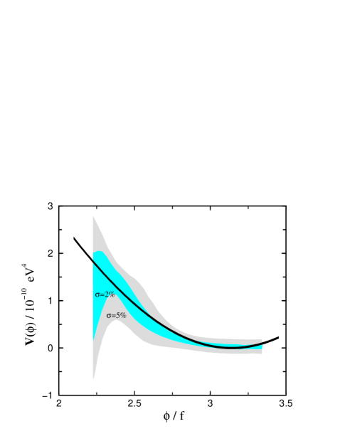
Figure 9: The 95% confidence interval for the reconstructed potential assuming luminosity distance errors of 5% and 2% (shaded areas) and the original potential (heavy line). For this reconstruction, $\Omega_{M}=0.3$ and $V(\phi)=V_{0}[1+\cos(\phi/f)]$ (from Huterer & Turner, 1998).

Both cosmologists and supernova theorists seem to use Eddington’s test to some degree. It seems to me that the summary of the SN Ia part of the meeting goes like this: We don’t know what SN Ia are; we don’t know how they work; but we believe SN Ia are very good standardizeable candles. I think what they mean is they have a general framework for understanding a SN Ia, the thermonuclear detonation of a Chandrasekhar mass white dwarf, and have failed in their models to find a second (significant) parameter that is consistent with the data at hand. Cosmologists are persuaded that the Universe is accelerating both because of the SN Ia results and because this was the missing piece to a grander puzzle.

Not only have SN Ia led us to the acceleration of the Universe, but also I believe they will play a major role in unraveling the mystery of the dark energy. The reason is simple: we can be confident that the dark energy was an insignificant component in the past; it has just recently become important. While, the anisotropy of the CBR is indeed a cosmic Rosetta Stone, it is most sensitive to physics around the time of decoupling. (To be very specific, the CBR power spectrum is almost identical for all flat cosmological models with the same conformal age today.) SNe Ia probe the Universe just around the time dark energy was becoming dominant (redshifts of a few). My student Dragan Huterer and I (Huterer & Turner, 1998) have been so bold as to suggest that with 500 or so SN Ia with redshifts between 0 and 1, one might be able to discriminate between the different possibilities and even reconstruct the scalar potential for the quintessence field (see Fig. 9).