Diffusion and scaling in escapes from two-degree-of-freedom Hamiltonian systems

Abstract

This paper summarises an investigation of the statistical properties of orbits escaping from three different two-degree-of-freedom Hamiltonian systems which exhibit global stochasticity. Each time-independent $H=H_{0}+{\epsilon}H^{\prime}$, with $H_{0}$ an integrable Hamiltonian and ${\epsilon}H^{\prime}$ a nonintegrable correction, not necessarily small. Despite possessing very different symmetries, ensembles of orbits in all three potentials exhibit similar behaviour. For ${\epsilon}$ below a critical ${\epsilon}_{0}$, escapes are impossible energetically. For somewhat higher values, escape is allowed energetically but still many orbits never escape. The escape probability $P$ computed for an arbitrary orbit ensemble decays towards zero exponentially. At or near a critical value ${\epsilon}_{1}>{\epsilon}_{0}$ there is a rather abrupt qualitative change in behaviour. Above ${\epsilon}_{1}$, $P$ typically exhibits (1) an initial rapid evolution towards a nonzero $P_{0}({\epsilon})$, the value of which is independent of the detailed choice of initial conditions, followed by (2) a much slower subsequent decay towards zero which, in at least one case, is well fit by a power law $P(t){\;}{\propto}{\;}t^{-\mu}$, with ${\mu}{\;}{\approx}{\;}0.35-0.40$. In all three cases, $P_{0}$ and the time $T$ required to converge towards $P_{0}$ scale as powers of ${\epsilon}-{\epsilon}_{1}$, i.e., $P_{0}{\;}{\propto}{\;}({\epsilon}-{\epsilon}_{1})^{\alpha}$ and $T{\;}{\propto}{\;}({\epsilon}-{\epsilon}_{1})^{\beta}$, and $T$ also scales in the linear size $r$ of the region sampled for initial conditions, i.e., $T{\;}{\propto}{\;}r^{-\delta}$. To within statistical uncertainties, the best fit values of the critical exponents ${\alpha}$, ${\beta}$, and ${\delta}$ appear to be the same for all three potentials, namely ${\alpha}{\;}{\approx}{\;}0.5$, ${\beta}{\;}{\approx}{\;}0.4$, and ${\delta}{\;}{\approx}{\;}0.1$, and satisfy ${\alpha}-{\beta}-{\delta}{\;}{\approx}{\;}0$. The transitional behaviour observed near ${\epsilon}_{1}$ is attributed to the breakdown of some especially significant KAM tori or cantori. The power law behaviour at late times is interpreted as reflecting intrinsic diffusion of chaotic orbits through cantori surrounding islands of regular orbits.

]

I INTRODUCTION

This paper summarises a study of the problem of escapes of energetically unbound orbits in strongly non-integrable two-degree-of-freedom Hamiltonian systems as an example of phase space transport in complex systems. This work has led to two significant conclusions: (1) When evolved into the future, ensembles of orbits of fixed energy often exhibit a rapid approach towards a constant escape probability $P_{0}$, the value of which is independent of the details of the ensemble and exhibits interesting scaling behaviour. Moreover, the values of the critical exponents appear to be relatively insensitive to the choice of Hamiltonian. (2) At later times, the escape probability decreases in a fashion which, for at least one model system, is well fit by a power law $P(t){\;}{\propto}{\;}t^{-\mu}$ with ${\mu}{\;}{\approx}{\;}0.35-0.40$. This nontrivial time-dependence is attributed to the fact that the possibility of escape to infinity is controlled by cantori, which can trap chaotic orbits near regular regions for extremely long times.

The first three papers in this series[1, 2, 3] (hereafter Papers $1$ - $3$) described a numerical investigation of the statistical properties of orbit ensembles evolving in nonintegrable two-degree-of-freedom Hamiltonian systems where it is possible energetically for trajectories to escape to infinity. Earlier investigations of individual orbits in these systems had led to two significant conclusions[4, 5]: (1) Just because escape is possible energetically does not mean that escape will inevitably occur; and, even if escape does occur, the time required for a trajectory to cross a Lyapunov curve[6] and hence escape to infinity may be very long compared with the natural crossing time. (2) In some phase space regions, the time and direction of escape vary smoothly as a function of initial conditions, but in other cases one discovers instead an apparent near-fractal dependence on the specific choice of initial data (cf.[7]).

This problem of escapes is an example of phase space transport in complex two-degree-of-freedom Hamiltonian systems, a subject which has been explored in detail over the past two decades (cf. [8, 9, 10, 11] and references cited therein). The passage of orbits through Lyapunov curves and their subsequent escape to infinity is the most conspicuous aspect of the transport, but crucial features of the bulk flow, especially at late times, appear to be controlled by diffusion through cantori[12, 13, 14, 15], which can trap orbits for very long times (cf. [9]). The chaotic behaviour of late escapers indicates that this problem is closely related to chaotic scattering (cf. [16, 17]), where an incident trajectory scatters to infinity at a time and in a direction that can exhibit a fractal dependence on the value of the impact parameter. However, the problem of escapes is also related to a variety of other physical problems, including, e.g., the dissociation of molecules (cf. [18]) or the evaporation of stars from a cluster (cf. [19]). Indeed, the phase space interpretation of the escape problem suggested in Section IV is completely consistent with the detailed phase space description deduced recently for escapes in the planar isoceles three-body problem.[20]

Paper I showed that, for at least one particular Hamiltonian system (the $H_{1}$ of eq. [1]), the microscopic chaos exhibited by individual orbits leads macroscopically to bulk regularities: (1) For sufficiently large deviations from integrability, localised ensembles of initial conditions evolve so as to exhibit a rapid approach towards a near-constant escape probability $P_{0}$, which is independent of the specific choice of initial conditions and which, if at all, only changes on a significantly longer time scale. (2) The value of $P_{0}$ scales in terms of an “order parameter” ${\epsilon}-{\epsilon}_{1}$. (3) For ensembles that probe a phase space region of specified size $r$, the time $T$ required to converge towards $P_{0}$ also scales in ${\epsilon}-{\epsilon}_{1}$. (4) For fixed values of ${\epsilon}-{\epsilon}_{1}$, $T$ also scales in the size $r$ of the phase space region sampled by the initial ensemble.

Subsequent work, summarised and extended here, has addressed several questions not considered in Paper 1:

(1) Do other potentials exhibit similar behaviour and, if so, are the scaling exponents the same? In other words, could this behaviour be universal?

(2) What happens at much later times? Does $P$ remain constant or is there a different asymptotic behaviour for larger values of $t$?

(3) Is there any obvious correlation between the time of escape for individual orbits in the ensemble and the exponential instability of those orbits, as probed, e.g., by short time Lyapunov exponents (cf.[21, 22, 23, 24])?

(4) Can one identify a simple, physically well motivated model to explain the observed behaviour?

This work is based on a detailed investigation of orbits in three different Hamiltonians, namely:

$$H_{1}={1\over 2}({\dot{x}}^{2}+{\dot{y}}^{2}+x^{2}+y^{2})-{\epsilon}x^{2}y^{2},$$

$$H_{2}={1\over 2}({\dot{x}}^{2}+{\dot{y}}^{2}+x^{2}+y^{2})-{\epsilon}xy^{2},$$

and

$$H_{3}={1\over 2}{\Biggl{(}}{\dot{x}}^{2}+{\dot{y}}^{2}+x^{2}+y^{2}-{2\over 3}y^{3}{\Biggr{)}}+{\epsilon}x^{2}y,$$

where ${\dot{x}}$ and ${\dot{y}}$ denote canonical momenta. In each case, the Hamiltonian is of the form

$$H=H_{0}+{\epsilon}H^{\prime},$$

with $H_{0}$ integrable and ${\epsilon}H^{\prime}$ a nonintegrable correction. ${\epsilon}$ is taken to be non-negative but is not assumed to be small. These Hamiltonians exhibit very different symmetries. $H_{1}$ is invariant under $x\to-x$ and/or $y\to-y$ and has four identical escape channels. $H_{2}$ is only symmetric with respect to $y\to-y$, and has two channels of escape. For ${\epsilon}=1$, $H_{3}$ reduces to motion in the Hénon-Heiles potential, which manifests a $2{\pi}/3$ rotation symmetry, but for ${\epsilon}>1$ this discrete symmetry is broken. Representative equipotential surfaces are exhibited in Fig. 1.

This research has led to four principal conclusions:

(1) For all three systems, there exists a critical ${\epsilon}_{1}$, larger than ${\epsilon}_{0}$, the smallest ${\epsilon}$ for which escapes can occur, which signals a qualitative change in short time behaviour: Below ${\epsilon}_{1}$ the escape probability $P$ decays towards zero exponentially, but for larger values of ${\epsilon}$ one observes instead an initial approach towards a near-constant nonzero $P_{0}$, the value of which is independent of the detailed choice of initial conditions.

2) For all three systems, $P_{0}$ scales in ${\epsilon}-{\epsilon}_{1}$, i.e., $P_{0}{\;}{\propto}{\;}({\epsilon}-{\epsilon}_{1})^{\alpha}$ with ${\alpha}>0$. For a uniform sampling of a given phase space region of fixed size $r$, the time $T$ required to converge towards $P_{0}$ also scales, i.e., $T{\;}{\propto}{\;}({\epsilon}-{\epsilon}_{1})^{-\beta}$, with ${\beta}>0$. For fixed ${\epsilon}$, $T$ also scales in the linear size $r$ of the phase space region initially sampled, i.e., $T{\;}{\propto}{\;}r^{-\delta}$ with ${\delta}>0$. Finally, the data are at least consistent with the possibility that the numerical values of ${\alpha}$, ${\beta}$, and ${\delta}$ are the same for all three potentials; and that ${\alpha}-{\beta}-{\delta}=0$.

(3) At later times, $P$ deviates from $P_{0}$ by exhibiting a slow decrease towards zero. For at least one Hamiltonian, namely $H_{3}$, this later time evolution is well fit by a power law $P{\;}{\propto}{\;}t^{-\mu}$, with a positive constant ${\mu}<1$.

(4) At least for $H_{3}$, and possibly for $H_{1}$ and $H_{2}$, orbits that escape early on tend to be more unstable than orbits which only escape at much later times, in that they have a larger short time Lyapunov exponent. Computed distributions of short time Lyapunov exponents and surfaces of section both support the hypothesis that the chaotic orbits divide, at least approximately, into relatively distinct subclasses, presumably separated by cantori.

The last two points suggest strongly that the late time evolution of $P(t)$ is controlled by cantori, which can trap chaotic orbits near regular islands for very long times. It is well known (cf. [9]) that cantori typically constitute the principal impediment for efficient phase space transport in two-degree-of-freedom systems and that diffusion through cantori is usually not characterised by a constant escape probability.

Section II describes the observed short time behaviour, summarising results presented in Papers 1 - 3 and discussing the evidence for universality. Section III focuses on longer time evolution, using surfaces of section and short time Lyapunov exponents to provide insights into flows associated with initially localised orbit ensembles. Section IV suggests a tentative physical interpretation of the numerical results in terms of flows in a chaotic phase space partitioned by cantori. Phase space is presumed to be dominated by “unconfined” chaotic orbits which, in the absence of any cantori or Lyapunov curves, would evolve towards a statistical equilibrium (cf. [11]). The constant $P_{0}$ observed at relatively early times is attributed to the fact that orbits sampling this near-equilibrium will escape at a near-constant rate. The decaying $P(t)$ later on reflects the fact that the phase space also includes an appreciable measure of temporarily “confined” or “sticky” (cf. [15, 26]) chaotic orbits which, albeit not trapped within the system forever, can only escape much later once they have breached one or more cantori to become unconfined.

II SHORT TIME BEHAVIOUR

A Description of the experiments

The experiments described here entailed a study of orbit ensembles with fixed energy $h$ evolving in $H_{1}$, $H_{2}$, and $H_{3}$ with variable ${\epsilon}$. Attention focused exclusively on ${\epsilon}>{\epsilon}_{0}(h)$, the smallest value of ${\epsilon}$ for which escape to infinity is possible energetically. The values of $h$ and ${\epsilon}_{0}$ for all three cases are given in Table 1.

Ensembles of initial conditions were generated by uniformly sampling a square cell of linear dimension $r$ in the $(x,{\dot{x}})$ plane, setting $y=0$, and then computing ${\dot{y}}={\dot{y}}(x,{\dot{x}},h)>0$. The cells were chosen to sample “interesting” phase space regions where most of the orbits do not escape at very early times. This implied that the time of escape for any given orbit typically manifested a sensitive dependence on initial conditions. Most of the computations involved a fiducial cell size $r=0.05$. However, when exploring the effects of varying cell size, cells as small as $r=1.0\times 10^{-4}$ were also used.

Each initial condition was integrated into the future and the location of the orbit on a Poincaré section noted at successive consequents, i.e., successive crossings of the $x=0$ phase space hyperplane with ${\dot{x}}<0$. If after consequent $t-1$ but before consequent $t$ the orbit crossed one of the Lyapunov curves, the orbit was recorded as having escaped at $t$. The experiments with $H_{1}$ [1, 4, 5] used a time series integrator. However, the experiments involving $H_{2}$ and $H_{3}$ [2, 3] exploited a more efficient Lie integrator truncated at twelfth order[27], which facilitated integrations of significantly larger ensembles typically containing $2000\times 2000$ initial conditions or more.

The fundamental object of interest is $P({\epsilon},t)$, the probability that a randomly chosen orbit is an escaping orbit with escape occuring between consequents $t-1$ and $t$. This escape probability, along with an estimated uncertainty ${\Delta}P({\epsilon},t)$, was defined by the obvious relation

$$P({\epsilon},t){\pm}{\Delta}P({\epsilon},t)={N_{esc}{\pm}\sqrt{N_{esc}}\over N_{tot}},$$

where $N_{esc}$ denotes the number of trajectories that escape between $t-1$ and $t$ and $N_{tot}$ the total number present at $t-1$.

B Results from the experiments

At early times, the escape probability can exhibit a complex, highly irregular behaviour, the details of which depend sensitively on the size and location of the initial cell. However, at somewhat later times, $P$ tends instead to exhibit a more systematic behaviour that is seemingly independent of the initial cell and depends only on the value of ${\epsilon}$. The qualitative form of this behaviour depends crucially on whether ${\epsilon}$ is above or below a critical ${\epsilon}_{1}>{\epsilon}_{0}$.

Below ${\epsilon}_{1}$, the escape probability $P({\epsilon},t)$ decays towards zero in a fashion that is well fit by an exponential. This is, e.g., illustrated in Figs. 2 a and b, which exhibit $P(t)$ and ${\rm ln}\,P(t)$ for one value of ${\epsilon}<{\epsilon}_{1}$ in $H_{2}$, namely ${\epsilon}=1.04$. The solid curve superimposes a best fit exponential $P{\;}{\propto}{\;}\exp(-t/{\tau})$, with ${\tau}=62.0$.

For ${\epsilon}>{\epsilon}_{1}$, $P({\epsilon},t)$ appears instead to converge towards a nonzero $P_{0}({\epsilon})$, the value of which depends on ${\epsilon}$ but is independent of the cell of initial conditions. The evidence is particularly compelling for $H_{1}$ and $H_{3}$, but somewhat weaker for $H_{2}$ where, especially for small ${\epsilon}-{\epsilon}_{1}$, the convergence is relatively slow and can merge into the later time evolution described in Section III. Examples of this behaviour are provided in Figs. 3 a-c, which exhibit $P(t)$ for representative values ${\epsilon}>{\epsilon}_{1}$ in $H_{1}$, $H_{2}$, and $H_{3}$. (Other examples are provided in Papers 1 - 3.) The transition at or near ${\epsilon}_{1}$ is quite abrupt and, for ${\epsilon}>{\epsilon}_{1}$, $P_{0}({\epsilon})$ is a monotonically increasing function of ${\epsilon}$. Moreover, for all three Hamiltonians one finds that, at least for relatively small values of the order parameter ${\epsilon}-{\epsilon}_{1}$, the escape probability $P_{0}({\epsilon})$ exhibits a simple scaling, namely [1, 2, 3]

$$P_{0}({\epsilon}){\;}{\propto}{\;}({\epsilon}-{\epsilon}_{1})^{\alpha},$$

with a constant ${\alpha}>0$. Illustrations of the goodness of fit of this scaling relation for the Hamiltonians $H_{1}$ and $H_{3}$ are provided, respectively, by Figs. 7 in Paper 1 and Figs. 4 in Paper 3, which exhibit plots of $P$ vs. ${\epsilon}$ and ${\rm ln}\,P$ vs. ${\rm ln}\,({\epsilon}-{\epsilon}_{1})$. The values of ${\epsilon}_{1}$ are again given in Table 1. That the escape probability approaches a roughly time-independent value can be interpreted by supposing that the cell of initial conditions has dispersed to fill certain large regions inside the Lyapunov curves in a nearly uniform fashion, and that trajectories are escaping near-randomly at a constant rate.

Using operational prescriptions described in Paper 1, one can also estimate the time $T$ required for an ensemble with ${\epsilon}>{\epsilon}_{1}$ to approach $P_{0}$. For cells of fixed size $r$, this $T$ appears to be roughly independent of initial conditions, depending only on ${\epsilon}$. Moreover, one finds that, for all three Hamiltonians, $T$ also scales in ${\epsilon}$ [1, 2, 3], i.e.,

$$T({\epsilon}){\;}{\propto}{\;}({\epsilon}-{\epsilon}_{1})^{-{\beta}},$$

with ${\beta}>0$. Illustrations of the goodness of fit of this scaling relation for the Hamiltonians $H_{1}$ and $H_{3}$ are provided, respectively, by Figs. 8 in Paper 1 and Figs. 5 in Paper 3, which exhibit plots of $T$ vs. ${\epsilon}$ and ${\rm ln}\,T$ vs. ${\rm ln}\,({\epsilon}-{\epsilon}_{1})$.

To the extent that a constant $P_{0}$ reflects a population that has dispersed throughout the regions inside the Lyapunov curves, one might anticipate that the convergence time $T$ would depend on the size $r$ of the initial cell, smaller cells approaching $P_{0}({\epsilon})$ more slowly. This too was confirmed numerically, Indeed, for all three Hamiltonians one finds that, for a fixed value of ${\epsilon}$, the convergence time $T(r)$ also scales in $r$ [1, 2, 3], i.e.,

$$T(r){\;}{\propto}{\;}r^{-\delta},$$

with ${\delta}>0$. This is illustrated in Figs. 9 and 10 of Paper 1 for two different values of ${\epsilon}$ for the Hamiltonian $H_{1}$.

It is obviously important to determine how abrupt the transition at ${\epsilon}{\;}{\approx}{\;}{\epsilon}_{1}$ actually is. However, this is difficult numerically. Eq. (7) implies that $T({\epsilon})$ diverges for ${\epsilon}\to{\epsilon}_{1}$, but this critical slowing down implies an intrinsic limitation in one’s ability to probe the details near the transition point.

C Possible evidence for universality

That the scaling relations (6) - (8) hold for all three Hamiltonians is clearly interesting. Even more striking, however, is the fact that, as is evident from Table 1, the values of the exponents ${\alpha}$, ${\beta}$, and ${\delta}$ are very similar for all three systems. In each case,

$${\alpha}{\;}{\sim}{\;}0.5,\hskip 14.45377pt{\beta}{\;}{\sim}{\;}0.4,\hskip 14.45377pt{\rm and}\hskip 14.45377pt{\delta}{\;}{\sim}{\;}0.1.$$

The uncertainties in ${\alpha}$ are dominated by uncertainties in the correct value of ${\epsilon}_{1}$. As discussed in Paper 1, because of the aforementioned critical slowing down ${\epsilon}_{1}$ is best estimated by looking at somewhat higher values of ${\epsilon}$ and extrapolating to smaller ${\epsilon}$. The uncertainties in ${\beta}$ are dominated by the precise prescription used to identify a convergence time. In particular, even though it is usually easy to determine a lower bound on the convergence time, the determination of an upper bound proves more difficult. It follows that the quoted error bars in Table 1 can be asymmetric. As regards the best fit ${\delta}$, there are two principal sources of uncertainty, namely (1) that the effect is relatively small (so that the fractional error is large) and (2) that, especially for very small values of $r$, different ensembles can exhibit significant variability.

Given these uncertainties, one cannot conclude unambiguously that ${\alpha}$, ${\beta}$, and ${\delta}$ are strictly equal for all three Hamiltonians. However, one can conclude that they are all comparable in size for all three systems and that, consistent with the uncertainties, they may in fact be equal.

It is also true that, to within statistical uncertainties,

$${\alpha}-{\beta}-{\delta}{\;}{\approx}{\;}0.$$

For $H_{1}$ and $H_{3}$ the evidence for this assertion is relatively strong. For $H_{2}$ the case is somewhat weaker, largely because the best fit ${\beta}$ is somewhat larger than for the other two systems. However, it should be noted that the error bars on the ${\beta}$ for $H_{2}$ are especially big. This reflects the fact that, for this system, the short time behaviour described in this Section merges relatively quickly into the later time evolution described in Section III, where $P(t)$ begins to decay to values below $P_{0}$. For $H_{1}$ and $H_{3}$ this subsequent decay only become significant at somewhat later times, at least for larger values of ${\epsilon}-{\epsilon}_{1}$.

The evidence for universality summarised here is certainly much weaker than for the universality first identified by Feigenbaum[28] for one-dimensional maps or by Escande and Doveil[29] and MacKay[30] in their renormalisation group analyses of tori, but it is, nevertheless, intriguing. Moreover, certain points are seemingly unambiguous. (1) For all three Hamiltonians, there is clear evidence for an abrupt change in behaviour at or near some critical value ${\epsilon}_{1}$. (2) For ${\epsilon}>{\epsilon}_{1}$, orbit ensembles evolve towards an escape probability $P(t)$ which is (a) largely independent of the choice of initial ensemble and (b) nearly time-independent, at least for relatively short times. (3) The convergence time $T$ depends both on cell size $r$ and ${\epsilon}-{\epsilon}_{1}$, larger cells and larger ${\epsilon}-{\epsilon}_{1}$ leading to a more rapid convergence. (4) Because $T({\epsilon},r)$ increases with decreasing ${\epsilon}-{\epsilon}_{1}$, pinning down the precise value of ${\epsilon}_{1}$ is quite hard. (5) The resulting uncertainties in ${\epsilon}_{1}$ do not impact the apparent fact that $P$ and $T$ scale in ${\epsilon}-{\epsilon}_{1}$. However, they do impact estimates of the precise values of ${\alpha}$, ${\beta}$, and ${\delta}$, thus making it difficult to determine whether these exponents are the same for all three potentials. What is clear is that, for all three potentials, the values of the exponents are comparable in magnitude.

III PHASE SPACE FLOW AT LATER TIMES

A Late time evolution of $P(t)$

Section II summarised experiments indicating that, on a relatively short time scale, the escape probability $P(t)$ evolves towards a near-constant value $P_{0}({\epsilon})$. However, there is no reason to expect that $P$ will remain approximately constant if the orbit ensembles are evolved for much longer times. If, e.g., the initial ensembles contain a few regular orbits that cannot escape, these will eventually dominate the orbits that remain in the system and $P(t)$ must decay towards zero exponentially. Even if the initial ensembles contain no regular orbits that never escape, one might anticipate more complicated behaviour at late times. If, e.g., some small subset of the chaotic escape orbits are stuck by cantori near some regular island for relatively long times, the escape probability should decrease below the initial near-constant $P_{0}$ once the other chaotic orbits have almost all escaped.

Such a decrease was first noted for orbit ensembles in $H_{2}$ and subsequently studied more systematically for ensembles in $H_{3}$ [3]. The principal conclusion is that, at least for ${\epsilon}>{\epsilon}_{1}$, when orbit ensembles are evolved for somewhat longer times the probability $P(t)$ begins to exhibit a slow, monotonic decrease. This is illustrated in Fig. 4 which, for one ensemble evolved in $H_{3}$, exhibits $P(t)$ for an ensemble with ${\sim}{\;}1.1\times 10^{9}$ orbits carefully chosen from a tiny region of size $r=1\times 10^{-5}$ to be dominated by “slow escapers,” so that $P(t)$ can be tracked for a comparatively long interval. Visually, $P(t)$ decays too slowly, and has the wrong curvature, to be well fit by an exponential. However, as is illustrated in Fig. 4b, which plots ${\rm ln}\,P$ as a function of ${\rm ln}\,t$, the data for $5<t<180$ or so can be fit quite well by a power law,

$$P(t){\;}{\propto}{\;}t^{-{\mu}},$$

with ${\mu}=0.39{\pm}0.02.$

This algebraic decay seems very robust, with ${\mu}$ apparently independent of the initial cell and, at least within a limited range, the value of ${\epsilon}$. The best fit value for several different values of ${\epsilon}$ (most of which were sampled for shorter times with far fewer orbits) is ${\mu}=0.35{\pm}0.07$.

B Tools of analysis

To ascertain why $P(t)$ changes in time and to better understand the qualitative character of the flow, orbit ensembles evolved in $H_{3}$ were also analysed in two other ways.

The first involved computing surfaces of section for an evolving ensemble. Each orbit in the ensemble was integrated into the future and, provided that it had not yet escaped, its values of $y$ and ${\dot{y}}$ were recorded at successive consequents and sorted to generate sequences of surfaces of section exhibiting $(y,{\dot{y}})$ pairs.

Such surfaces of section allow one to determine the extent to which the ensemble has evolved to cover a large portion of the allowed phase space. Moreover, they can facilitate the detection of “zones of avoidance” associated with regular islands and/or with orbits that have immediately escaped, as well as phase space regions with excess concentrations of orbits, corresponding presumably to regions from which escape is especially difficult.

The second involved computing short time Lyapunov exponents (cf. [21, 22, 23, 24]), which probe the average exponential instability of chaotic orbits over finite time intervals. By analogy with ordinary Lyapunov exponents, a finite time ${\chi}(t)$ can be defined by the obvious prescription

$${\chi}(t)=\lim_{{\delta}Z(0)\to 0}{1\over t}\ln{|{\delta}Z(t)|\over|{\delta}Z(0)|}$$

where $|{\delta}Z|^{2}=({\delta}x)^{2}+({\delta}y)^{2}+({\delta}{\dot{x}})^{2}+({\delta}{\dot{y}})^{2}$ denotes the magnitude of the initial phase space perturbation, defined with respect to the natural Euclidean norm. These exponents were determined computationally in the usual way [25] by introducing a small initial perturbation ${\delta}x(0)=1\times 10^{-12}$ in the $x$-direction and evolving simultaneously both the perturbed and unperturbed orbits, periodically renormalising the amplitude of the perturbation to assure that $|{\delta}Z(t)|$ remains smaller than $1\times 10^{-8}$.

At early times, the ${\chi}(t)$ computed in this way will depend strongly on the initial perturbation. However, if the orbit segment is chaotic, ${\chi}(t)$ will quickly become dominated by the component of the perturbation in the most unstable direction and become relatively insensitive to the initial ${\delta}Z(0)$. Note also that, given ${\chi}(t)$ for two different times, $t_{1}$ and $t_{2}$, one can identify the average exponential instability for the interval $t_{1}<t<t_{2}$ as

$${\chi}(t_{2}-t_{1})={t_{2}{\chi}(t_{2})-t_{1}{\chi}(t_{1})\over t_{2}-t_{1}}.$$

Short time Lyapunov exponents were used to confirm that, for the values of $h$ and ${\epsilon}$ under consideration, most, if not all, of the computed orbits in $H_{3}$ are chaotic. Distributions of short time Lyapunov exponents were also used to show (1) that the chaotic orbits which have not escaped often appear to divide into distinct populations and (2) that there are correlations between the magnitude of ${\chi}$ and the time at which the orbit escapes.

C Surfaces of section

Figures 5 a-f exhibit a sequence of sections, generated for one ensemble at six different consequents, $t=2$, $6$, $10$, $15$, $20$, and $25$. This ensemble was comprised of $160,000$ orbits evolved with ${\epsilon}=1.13$, a value only marginally above the critical ${\epsilon}_{1}$. The cell of initial conditions, with $0<x<0.05$, $0.04<{\dot{x}}<0.09$, $y=0$, $h=1/6$, and hence $0.5681<{\dot{y}}<0.5780$ is located near the top of the energetically accessible portion of the surface of section. The first escapes occured at $t=4$, and the largest number of escapes was at $t=7$. $P(t)$ first settled down towards a smoothly varying form around $t=10-12$.

Inspection of these, and other intermediate, sections indicates that the orbits remaining inside the Lyapunov curves tend systematically to spread over a relatively large fraction of the energetically allowed phase space. Indeed, the elongated striae associated with the specific choice of initial conditions, so conspicuous at consequents $t=2$ and $6$, have been significantly blurred by $t=10$ and have nearly disappeared by $t=25$.

For $t<6-8$, the form of the sections is strongly time-dependent. However, by $t=10$ the ensemble has evolved to yield sections characterised by three seemingly distinct regions which persist to later times, namely: (1) two large holes accompanied by smaller surrounding whorls, (2) several overdense regions at positive values of $y$, and (3) a larger region characterised by a substantially lower density. As time passes, the occupied regions all decrease in density, but the overdense regions remain overdense.

The two holes and their surrounding whorls are associated with escapes through Lyapunov curves: any orbit with values of $y$ and ${\dot{y}}$ in these regions would already have escaped before intersecting the $x$-axis. For larger values of ${\epsilon}$ it is apparent that the visible whorls are part of an elaborate set of structures that penetrate throughout large portions of the lower density regions, and that this lower density region, which appears macroscopically to be populated in a near-uniform fashion, is really laced with tiny zones of avoidance.

Assuming that essentially all the orbits in the ensemble are chaotic, the overdense regions can be interpreted as reflecting trapping near regular islands: Even though these islands may be so small as to be almost unobservable, cantori can significantly impact relatively large portions of the chaotic phase space[9, 11]. The idea then is that orbits in the overdense regions are trapped by cantori and can only escape once they have diffused through the cantori and can travel unimpeded throughout the remainder of the chaotic sea.

The existence of this three-part structure – holes, less dense regions, and more dense regions – is independent of the choice of initial conditions. Moreover, the general locations of the holes and the higher density regions are insensitive to the precise value of ${\epsilon}$. This latter fact is manifested in Fig. 6, which shows the analogue of Fig. 5 c, now generated for an ensemble with ${\epsilon}=1.06$. This reinforces the interpretation that one is seeing the effects of basic phase space structures, rather than transient streaming motions reflecting the choice of ensemble.

D Short time Lyapunov exponents

Perhaps the most obvious way to search for correlations between the degree of exponential instability exhibited by a chaotic orbit and the time at which it escapes is to compute the mean short time Lyapunov exponent, ${\langle}{\chi}(t_{E}){\rangle}$, for all the orbits in an ensemble that escape between successive consequents $t_{E}$ and $t_{E}+1$. The results of one such computation are presented in Fig. 7, which was generated from an ensemble of $1\times 10^{\,6}$ orbits evolved in $H_{3}$ with ${\epsilon}=1.30$. ${\langle}{\chi}(t_{E}){\rangle}$ clearly exhibits an initial relatively rapid decrease for $t_{E}<5-10$, followed by a more extended period during which ${\langle}{\chi}(t_{E}){\rangle}$ decreases more slowly. (The initial point in Fig. 7 at $t_{E}=5$ is statistically significant.)

As described above, interpreting the computed ${\langle}{\chi}(t_{E}){\rangle}$ at very early times as an accurate probe of the average maximum short time exponent is suspect. Given, however, that the typical values of ${\chi}$ are greater than or of order unity, the computed ${\langle}{\chi}(t_{E}){\rangle}$ should be relatively reliable for $t_{E}>5$ or so, which means that the initial rapid decrease is most likely real. It is not completely clear whether ${\langle}{\chi}(t_{E}){\rangle}$ will continue to decrease at late times, or whether it asymptotes towards a nonzero value. However, the existence of a continued decrease out to at least $t=70$ or so is unquestionably significant statistically.

The observed decrease in ${\langle}{\chi}(t_{E}){\rangle}$ can be easily interpreted by assuming that the chaotic phase space inside the Lyapunov curves divides into two different regions, namely (1) a region where orbit segments are less unstable exponentially and from which direct escape to infinity is difficult, if not impossible, and (2) a region where orbit segments are more unstable and from which escape to infinity can proceed on a relatively short time scale. The idea is that orbits which remain inside the Lyapunov curves for a long time will typically spend most of their time in the less unstable region before entering the more unstable region and subsequently escaping to infinity. It follows that, for orbits that only escape at late times, the short time exponent ${\chi}(t_{E})$, which probes the average instability for $0<t<t_{E}$, will typically be smaller than for early escapers.

Suppose, oversimplistically, that orbit segments in the less and more unstable regions can be characterised respectively by unique short time exponents ${\chi}_{L}$ and ${\chi}_{H}$, and that any orbit that enters the high ${\chi}$ region will escape after exactly a time $t_{e}$. It then follows from eq. (13) that the total ${\chi}(t_{E})$ for an orbit escaping at time $t_{E}$ satisfies

$${\chi}(t_{E})={1\over t_{E}}{\Bigl{[}}t_{e}\,{\chi}_{H}+(t_{E}-t_{e})\,{\chi}_{L}{\Bigr{]}}.$$

Consistent with Fig. 7, this implies that ${\chi}(t_{E})$ decreases monotonically, but eventually asymptotes towards a nonzero ${\chi}_{L}$. For $t_{E}>15$ or so the computed ${\langle}{\chi}(t_{E}){\rangle}$ exhibited in Fig. 7 is in fact well fit by eq. (14) with ${\chi}_{L}=0.92$ and $t_{e}({\chi}_{H}-{\chi}_{L})=7.80$.

To confirm that the observed decrease in ${\langle}{\chi}(t_{E}){\rangle}$ reflects transitions between relatively distinct orbit populations, it is also instructive to determine how short time Lyapunov exponents computed for the same set of orbits change as a function of time. One way to do this is to consider all the orbits in an initial ensemble that escape at a given time $T_{E}$ and, given expressions for ${\chi}(t)$ for times $t<T_{E}$, computed using eq. (12), extract short time exponents for different intervals $t_{1}<t<t_{2}$.

Figure 8, generated from the same ensemble as Fig. 7, focuses on all $832$ orbits that escaped at $t=50$, computing distributions of short time exponents for the intervals $15<t<20$ (solid curve) and $45<t<50$ (dashed curve). Both distributions are bimodal, seemingly comprised of two different populations with peaks at or near the same values of ${\chi}$, but it is clear that the relative height of the two peaks changes significantly in time. For the earlier interval, the lower ${\chi}$ population dominates whereas for the later interval the low and high ${\chi}$ populations are of more nearly equal importance. For $10<t<15$ the mean ${\langle}{\chi}{\rangle}=0.70$; for $45<t<50$ the mean ${\langle}{\chi}{\rangle}=1.11$. This is consistent with the interpretation that most of the orbits that escaped at $t=50$ were members of a low ${\chi}$ population at early times but shifted to the higher ${\chi}$ population shortly before escaping from the system.

IV PHYSICAL INTERPRETATION

A General considerations

This section suggests a simple model for the behaviour observed in Sections II and III which is based on the assumption that, over finite intervals, orbits divide at least approximately into three distinct classes, namely (1) regular orbits, (2) sticky, or temporarily confined, orbits, and (3) unconfined chaotic orbits, even though the distinction between confined and unconfined chaos disappears entirely in the $t\to\infty$ limit.

Conventional wisdom would suggest that the presence of stable periodic orbits, which one expects for generic Hamiltonians, implies that there must exist a finite measure of regular orbits, even at very high energies $h$ and/or large values of ${\epsilon}$. However, the existence of such regular regions, separated from the remaining chaotic orbits by invariant KAM tori, suggests in turn that the surrounding chaotic sea should contain cantori which, albeit not impenetrable barriers, can trap chaotic orbits near the regular islands for relatively long intervals of time. Even if there is no absolute distinction between different types of orbits in the chaotic sea, there may exist short time de facto distinctions which can have significant implications for the Hamiltonian flow. (Strictly speaking, in general there will also exist a finite measure of chaotic orbits inside the KAM tori. However, these can never breach the invariant tori and, as such, will never be able to escape to enter the surrounding stochastic sea. For this reason, they may be lumped together with the regular orbits in the following discussion.)

If a localised ensemble of phase space points, each corresponding to a chaotic orbit with energy $h$, is evolved in a time-independent potential which, as for the Hamiltonians (1) - (3) for ${\epsilon}<{\epsilon}_{0}$, has a compact constant energy hypersurface, one anticipates a coarse-grained evolution towards an invariant distribution corresponding to a uniform population of the accessible phase space[11]. Numerical experiments suggest (cf. [31]) that, if the chaotic phase space is not significantly impacted by cantori, so that a single chaotic orbit can easily access the entire region without having to diffuse through any barriers (cf. [32, 33]), this approach will proceed exponentially in time on a time scale of order the natural crossing time, $t_{cr}$. If, however, cantori play an important role in partitioning the chaotic phase space regions over relatively short time scales, one can instead observe a more complex, seemingly two stage process [32, 33, 34]. Sets of orbits in different nearly disjoint regions will rapidly approach near-invariant distributions, corresponding to near-uniform populations of the separate regions; but only later, on a significantly longer time scale, will orbits from different regions “mix” to yield an approach towards a true invariant distribution.

Suppose now that ${\epsilon}>{\epsilon}_{0}$, so that orbits are no longer bound energetically. It then seems reasonable to interpret the observed behaviour of orbits in terms of two distinct sorts of “escape,” namely (1) unconfined chaotic orbits which pass through Lyapunov curves to escape to infinity and (2) confined chaotic orbits, originally stuck near the regular regions, which pass through one or more cantori to become unconfined, after which they too can escape to infinity. To the extent that the escape channels – both the simple gaps breached by Lyapunov curves and the more complex cantor sets of holes in cantori – are small, or that one is considering phase space regions relatively far from the escape channels, it should be reasonable to visualise what is happening in terms of ensembles that have evolved towards a near-invariant distribution.

Suppose, in particular, that one selects an initial ensemble where most of the orbits are unconfined chaotic, but that there are also a significant number of confined chaotic orbits and, perhaps, a few regular orbits. It is then easy to explain the qualitative evolution.

On a relatively short time scale, the unconfined chaotic orbits should evolve towards a near-uniform population of the phase space regions far from the Lyapunov curves and outside any cantori which significantly impede phase space transport. (The fact that, in the late time sections of Fig. 5, different parts of the lower density region seem to have the same relative density at different times supports this idea.) However, once this near-invariant distribution has been achieved, escapes to infinity should proceed “at random” at a near-constant rate, so that the unconfined chaotic orbits will be characterised by a constant escape probability. To the extent that the total orbit population is dominated by the initially unconfined orbits, and that appreciable numbers of confined orbits have not yet become unconfined, the total escape probability $P$ should be approximately constant.

Eventually, however, most of the unconfined chaotic orbits will have escaped, so that, assuming that unconfined orbits cross the Lyapunov curves more quickly than confined orbits diffuse through cantori, the total escape probability is impacted significantly, and ultimately dominated, by the remaining orbits. If all these orbits were regular and unable to escape, one would expect $P$ to decay exponentially in time (cf. [1]). Given, however, that most of the remaining orbits are chaotic orbits originally trapped by cantori, as seems true for ${\epsilon}>{\epsilon}_{1}$, one expects a slower decay in $P$ reflecting transitions from confined to unconfined chaos: The idea here is that confined orbits will only diffuse through cantori to become unconfined very slowly, but that, once unconfined, they will quickly escape to infinity. The observed $P{\;}{\propto}{\;}t^{-\mu}$ is thus driven by the diffusion of orbits through cantori rather than their escape through Lyapunov curves. That diffusion through cantori need not characterised by a constant escape probability is in fact well known (cf. [9]).

The same qualitative picture should remain valid even if the initial orbit ensemble is carefully selected to contain no chaotic orbits trapped near the regular regions. Even if most of the original unconfined orbits quickly escape to infinity through one of the Lyapunov curves, a small fraction of those orbits could become trapped by cantori. However, once trapped most of these orbits will only leak out at significantly later times, when the population of unconfined orbits inside the Lyapunov curves has become significantly reduced.

B A simple model

Consider an ensemble of initial conditions of energy $h$, located inside the Lyapunov curves, which may be divided into three different classes – unconfined chaotic, temporarily confined chaotic, and regular – characterised by numbers $N_{u}(0){\;}{\gg}{\;}{\hat{N}}_{c}(0){\;}{\gg}{\;}N_{r}(0)$. Now implement a probabilistic description, treating the regular orbits as a separate population that can never escape, but allowing for three sorts of transitions, namely escapes of unconfined orbits through Lyapunov curves, trapping of unconfined orbits by cantori, and leakage of confined orbits to become unconfined orbits inside the Lyapunov curves.

Calculating the total escape rate $R$, the continuum limit of the discrete probability $P$ computed in the numerical experiments summarised above, is straightforward if one makes two basic assumptions, each implicit in the preceding and seemingly consistent with the numerical experiments. (1) The rate at which unconfined orbits escape to infinity assumes a constant value ${\lambda}$, independent of time. (2) ${\lambda}$ is much larger than the rates at which unconfined orbits become temporarily confined and temporarily confined orbits become unconfined.

These assumptions imply that, at early times, the total escape rate is dominated by the escape of initially unconfined orbits, and that the details of any early trapping of unconfined orbits are irrelevant. This means that, when computing the total escape rate, the confined population may be approximated by an expression of the form

$$N_{c}(t)=N_{c}(0)f(t),$$

where $N_{c}(0)$ allows for a possible early time trapping of some small fraction of the originally unconfined orbits and $f(t)$ is a monotonically decreasing function of time, assumed to satisfy an initial condition $f(0)=1$. The rate $R_{cu}$ at which temporarily confined orbits become unconfined is thus

$$R_{cu}(t)=-{1\over f}{df\over dt}$$

Similarly, $N_{u}(t)$ must satisfy a simple rate equation

$$\hskip-28.90755pt{dN_{u}(t)\over dt}={dN_{u}(t)\over dt}{\Biggl{|}}_{out}+{dN_{u}(t)\over dt}{\Biggl{|}}_{in}$$

$$=-{\lambda}N_{u}(t)-N_{c}(0){df(t)\over dt}.$$

This latter equation is easily solved to yield

$$N_{u}(t)=N_{u}(0)e^{-{\lambda}t}-N_{c}(0)\,\int_{0}^{t}\,d{\tau}e^{{\lambda}({\tau}-t)}\;{df({\tau})\over d{\tau}}\;.$$

However, this implies that the total escape rate

$$R(t){\;}{\equiv}{\;}{-1\over(N_{r}+N_{c}+N_{u})}{\;}{d\over dt}(N_{r}+N_{c}+N_{u})$$

$$={{\lambda}{\Bigl{[}}1-{\nu}_{c}\,\int_{0}^{t}\,d{\tau}e^{{\lambda}{\tau}}df({\tau})/d{\tau}{\Bigr{]}}\over{\Bigl{[}}1-{\nu}_{c}\,\int_{0}^{t}\,d{\tau}e^{{\lambda}{\tau}}df({\tau})/d{\tau}+{\nu}_{c}f(t)e^{{\lambda}t}+{\nu}_{r}e^{{\lambda}t}{\Bigr{]}}}\;,$$

where ${\nu}_{c}=N_{c}(0)/N_{u}(0)$ and ${\nu}_{r}=N_{r}/N_{u}(0)$ reflect original relative abundances.

That the escape rate through the Lyapunov curves in much larger than the rate at which confined orbits become unconfined means that ${\lambda}{\;}{\gg}{\;}|(1/f)(df/dt)|.$ This implies, however, that the integrals in the preceding equation can be evaluated perturbatively, expanding $df({\tau})/d{\tau}$ about its value at time ${\tau}=t$. Recognising that the second term in the denominator is small compared with the third, one thus concludes that

$$R(t){\;}{\approx}{\;}{{\lambda}-{\nu}_{c}e^{{\lambda}t}df(t)/dt\over 1+{\nu}_{c}e^{{\lambda}t}f(t)+{\nu}_{r}e^{{\lambda}t}}\;.$$

Granted that ${\nu}_{r}{\;}{\ll}{\;}{\nu}_{c}{\;}{\ll}{\;}1$, $R(t)$ typically admits three different, asymptotic regimes, namely

(1) an early time regime where $R{\;}{\approx}{\;}{\lambda}$;

(2) an intermediate regime where $R\to-(1/f)df/dt$; and

(3) a late time regime where $R\to-({\nu}_{c}/{\nu}_{r})df/dt$.

At early times, the total escape rate is fixed by the rate at which initially unconfined orbits cross the Lyapunov curves. Later, once most of these original unconfined orbits have escaped, $R(t)$ is set by the rate at which confined chaotic orbits become unconfined. Finally, once most of the initially confined orbits have escaped, there is a more rapid decrease in $R$ towards zero, reflecting the fact that the now dominant regular population can never escape.

It is natural to interpret the probability $P{\;}{\propto}{\;}t^{-{\mu}}$ described in Section III as reflecting the intermediate regime. If ${\mu}$ were equal to unity, one would then infer a population

$$N_{c}(t){\;}{\propto}{\;}t^{-q},$$

for some constant $q>0$, i.e., an eventual power law decay in the number of confined orbits. Given, however, that the best fit ${\mu}<1$, one infers instead a population

$$N_{c}(t){\;}{\propto}{\;}\exp(-qt^{1-\mu}),$$

which decays faster than an a power law but slower than the exponential decrease associated with a constant escape rate.

That $P(t)$ is not constant is hardly surprising. Indeed, diffusion through cantori, interpreted as orbits wending their way through a self-similar collection of turnstiles,[32, 33] would suggest that $P(t)$ decay in time (cf. [36, 37, 38]). Rather, what is interesting is that ${\mu}{\;}{\neq}{\;}1$. In the context of chaotic scattering, one seems to see a sharp distinction between hyperbolic scattering (cf. [17, 35]), where the number of incident particles remaining within the scattering region at time $t$ decays exponentially, i.e., $N(t){\;}{\propto}{\;}\exp(-{\lambda}t)$, and nonhyperbolic scattering (cf. [39]), where the number remaining decays as a power law, i.e., $N(t){\;}{\propto}{\;}t^{-q}$. The origin of the intermediate behaviour observed here is, at the present, unclear.

This picture presupposes that ${\nu}_{r}{\;}{\ll}{\;}{\nu}_{c}{\;}{\ll}{\;}1$. Indeed, if these inequalities fail, the qualitative evolution can change significantly. Suppose, for instance, that temporarily confined chaotic orbits are unimportant compared with regular orbits, so that one need consider only two orbit classes – regular and unconfined –, and that, even early on, there are many more regular than unconfined orbits. It then follows immediately that, already at early times, $R(t)$ should decay towards zero exponentially:

$$R(t){\;}{\approx}{\;}{{\lambda}\over 1+(N_{r}/N_{c}){\exp}(-{\lambda}t)}{\;}\to{\;}{N_{c}\over N_{r}}{\,}{\exp}(-{\lambda}t).$$

This is consistent with the observed behaviour for ${\epsilon}_{0}<{\epsilon}<{\epsilon}_{1}$ where, as noted already, $P(t)$ decays towards zero without first asymptoting towards a near constant nonzero value.

C Discussion

To place the preceding in an appropriate context, three important points should be noted.

1. Extracting a near-constant $P_{0}({\epsilon})$ is necessarily a somewhat imprecise operation. The algorithm described in Paper 1, or any obvious alternative, depends crucially on the idea that $P(t)$ will evolve towards a form that is largely independent of the initial conditions on a time scale sufficiently short that appreciable numbers of sticky chaotic orbits do not escape and the total escape probability is dominated by the near-constant rate at which unconfined orbits escape. If the ensemble “forgets” its initial conditions sufficiently quickly, it is possible operationally to identify a reasonable estimate of $P_{0}({\epsilon})$. Strictly speaking, however, the ensemble is really evolving towards a characteristic $P({\epsilon},t)$ which manifests a slow, but nontrivial, time-dependence. This leads to an inherent inaccuracy in the determination of the values of the critical ${\epsilon}_{1}$ and, especially, the exponents ${\alpha}$, ${\beta}$, and ${\delta}$.

2. The calculations described in Section III were restricted to relatively short times, $t<200$ or so; and, for this reason, one cannot preclude the possibility that, on a significantly longer time scale, $P(t)$ could assume a form very different from what was suggested in Section IV. For example, one cannot preclude the possibility that, for much later times, $P(t){\;}{\propto}{\;}t^{-1}$, in agreement with Karney’s [37] experiments. Ideally one might like to integrate for much longer times, but this quickly becomes very expensive computationally: because the overwhelming majority of the orbits in an initial ensemble escape relatively early on, one would need to start with an absolutely enormous collection of initial conditions in order to derive statistically significant conclusions about behaviour at much later times. Nevertheless, even though one cannot exclude the possibility of different later time behaviour, it is significant that the observed scaling $P(t){\;}{\propto}{\;}t^{-\mu}$ for $t<180$ or so appears to be robust

It should also be noted that one cannot completely exclude the possibility that the long time integrations described in Section III are contaminated by accumulating errors which, e.g., make the system slightly dissipative. Numerical tests described in Paper I allow one to be confident that the early time computations ($t<20$ or so) are reliable, but there is less hard evidence to justify accepting long time integrations at face value. All that can be said definitively is that, even for the longest time integrations, the relative energy error for an orbit was never larger than $2\times 10^{-8}$ and usually orders of magnitude smaller.

3. This simple three-component model, based on two, and only two, nearly distinct classes of chaotic orbits, may well be oversimplistic. Indeed, lumping together every chaotic orbit that is not unconfined into a single population assumed to have reached a statistical near-equilibrium seems less justified than assuming that, at least away from the Lyapunov curves, the unconfined phase space is characterised by a near-invariant distribution. Furthermore, the entire analysis assumes an abrupt transition occuring at or near some critical ${\epsilon}_{1}$. However, one can argue that these limitations are not completely unreasonable. Detailed examinations of orbit ensembles on a compact phase space hypersurface indicate that, oftentimes, many of the qualitative features of a flow can be interpreted by allowing only for two classes of chaotic orbits, named sticky and unconfined (cf. [34, 32, 33]). Moreover, investigations of the effects of increasing deviations from integrability suggest that, as the control parameter ${\epsilon}$ becomes larger, holes in cantori can abruptly increase in size, so that what was initially a barrier that could only be penetrated on a very long time scale ceases to play a significant role in impeding phase space transport [40].

TABLE I.: Critical escape parameters

	$H_{1}$	$H_{2}$	$H_{3}$
$h$	$0.12$	$0.125$	$1/6{\;}{\approx}{\;}0.167$
${\epsilon}_{0}$	$1/(4h){\;}{\approx}{\;}2.08$	$1/\sqrt{8h}=1.00$	$1.00$
${\epsilon}_{1}$	$4.90\pm 0.01$	$1.15^{+0.02}_{-0.05}$	$1.10{\pm}0.05$
${\alpha}$	$0.46{\pm}0.05$	$0.46{\pm}0.05$	$0.45{\pm}0.05$
${\beta}$	$0.39^{+0.14}_{-0.06}$	$0.50^{+0.15}_{-0.10}$	$0.37^{+0.10}_{-0.07}$
${\delta}$	$0.08{\pm}0.03$	$0.11{\pm}0.03$	$0.12{\pm}0.03$

FIG. 1.: Equipotential surfaces of the potential for (a) $H_{1}$ with ${\epsilon}=5.26$, (b) $H_{2}$ with ${\epsilon}=3.0$, and (c) $H_{3}$ with ${\epsilon}=1.0$. $O_{1}$, $O_{2}$, $O_{3}$ and $O_{4}$ represent Lyapunov unstable periodic orbits.

FIG. 2.: (a) The escape probability, $P(t)$, computed for five different cells of initial conditions evolved in $H_{2}$ with ${\epsilon}=1.04<{\epsilon}_{1}$. The solid curve is an exponential fitted to the interval $20<t<100$. The error bars reflect uncertainties computed as in eq. (5). (b) The same data on a log-log plot. Here the orbits from the different cells have been combined to yield a single $P$ and ${\Delta}P$, again computed as in eq. (5).

FIG. 3.: (a) The escape probability, $P(t)$, computed for several different cells of initial conditions in $H_{1}$ with ${\epsilon}=5.05>{\epsilon}_{1}$. The dashed line indicates the best fit $P_{0}$. (b) The same for $H_{2}$ with ${\epsilon}=1.20$. (c) The same for $H_{3}$ with ${\epsilon}=1.30$

FIG. 4.: (a) The escape probability, $P(t)$, computed for the same initial conditions as in Fig. 3 (c), now allowing for much longer times. The solid curve exhibits a power law fit, $P{\;}{\propto}{\;}t^{-\mu}$, with ${\mu}=0.39.$ (b) The same data on a semilog plot, analysed as for Fig. 2b.

.

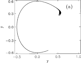
FIG. 5.: (a) Surface of section at $t=2$ for an ensemble of initial conditions evolved in $H_{3}$ with ${\epsilon}=1.13$, exhibiting $y$ and $\dot{y}$ for every orbit still inside the Lyapunov curves that crosses the $x=0$ axis with ${\dot{x}}<0$ between consequents $t$ and $t+1$.

(b) The same for $t=6$.

(c) The same for $t=10$.

(d) The same for $t=15$.

(e) The same for $t=20$.

(f) The same for $t=25$.

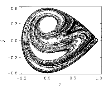
FIG. 6.: A surface of section analogous to Fig 5 c, generated at $t=10$ for an ensemble of orbits with ${\epsilon}=1.06$.

FIG. 7.: (a) The escape probability, $P(t)$, computed for the same initial conditions as in Fig. 3 (c), now allowing for much longer times. The solid curve exhibits a power law fit, $P{\;}{\propto}{\;}t^{-\mu}$, with ${\mu}=0.37.$ (b) The same data on a semilog plot, analysed as for Fig. 2b.

FIG. 8.: Distributions of short time Lyapunov exponents for the intervals $15<t<20$ (solid curve) and $45<t<50$ (dashed curve) for orbits that escape through the Lyapunov curves at consequent $t=50$.