A New Shear Estimator for Weak Lensing Observations

Abstract

We present a new shear estimator for weak lensing observations which properly accounts for the effects of a realistic point spread function (PSF). Images of faint galaxies are subject to gravitational shearing followed by smearing with the instrumental and/or atmospheric PSF. We construct a ‘finite resolution shear operator’ which when applied to an observed image has the same effect as a gravitational shear applied prior to smearing. This operator allows one to calibrate essentially any shear estimator. We then specialize to the case of weighted second moment shear estimators. We compute the shear polarizability which gives the response of an individual galaxy’s polarization to a gravitational shear. We then compute the response of the population of galaxies, and thereby construct an optimal weighting scheme for combining shear estimates from galaxies of various shapes, luminosities and sizes. We define a figure of merit — an inverse shear variance per unit solid angle — which characterizes the quality of image data for shear measurement. The new method is tested with simulated image data. We discuss the correction for anisotropy of the PSF and propose a new technique involving measuring shapes from images which have been convolved with a re-circularizing PSF. We draw attention to a hitherto ignored noise related bias and show how this can be analyzed and corrected for. The analysis here draws heavily on the properties of real PSF’s and we include as an appendix a brief review, highlighting those aspects which are relevant for weak lensing.

1 Introduction

Weak lensing provides a probe of the dark matter distribution on a range of scales from galaxy halos, through clusters of galaxies, to large-scale-structure (see e.g. the recent review of ?), and references therein). In the weak lensing or thin lens approximation, the effect of gravitational lensing on the image of a distant object is a mapping of the surface brightness:

$$f^{\prime}(r_{i})=f((\delta_{ij}-\psi_{ij})r_{j})$$ (1)

where the 2-vector $r_{i}$ is the angular position on the sky measured relative to the center of the image, $f$ is the intrinsic surface brightness that would be seen in the absence of lensing, and the symmetric ‘distortion tensor’ $\psi_{ij}$ is an integral along the line of sight of the transverse second derivatives of the gravitational potential $\Phi$ Gunn (1967). In an open cosmology, for instance, the distortion for an object at conformal distance $\omega_{s}$ can be written as

$$\psi_{lm}=2\int d\omega{\sinh\omega\sinh(\omega_{s}-\omega)\over\sinh\omega_{s}}\partial_{l}\partial_{m}\Phi$$ (2)

(Bar-Kana (1996); Kaiser (1998)) where $\partial_{i}\equiv\partial/\partial x_{i}$ and $x_{i}=\theta_{i}\sinh\omega$ with $\theta_{i}$ being a 2-component Cartesian vector in the plane of the sky and where the potential is related to the density contrast by $\nabla^{2}\Phi=4\pi G\delta\rho$, the Laplacian here being take with respect to proper spatial coordinates. Equation (2) can be generalized to deal with sources at a range of distances, and with either accurately known redshifts or partial redshift information from broadband colors.

The distortion will, in general, change both the shapes and sizes, and hence luminosities, of distant objects. Any component of the distortion which is coherent over large scales — larger than the typical angular separation of background galaxies — is therefore potentially observable as a relative modulation of the counts of objects or as a statistical anisotropy of the galaxy shapes, and this allows one to constrain the fluctuations in the total density $\delta\rho$ on the corresponding scales. Here we will focus on analysis of shape anisotropy, or ‘image shear’, though the methodology is readily extendible to include the effects of magnification.

While the effect of a shear on the sky surface brightness (1) is rather simply stated, no completely satisfactory method for estimating the distortion has yet emerged. Perhaps ideally one would attack this problem using likelihood; that is, one would ask: what is the probability to observe a given set of background galaxy images given that they are drawn from some statistically isotropic unlensed parent distribution, as a function of the parameters $\psi_{lm}$. Unfortunately, this does not seem to be a particularly tractable problem. Also, the problem is further complicated by the finite resolution of real observations, and by noise in the images. Instead, what has been done is to adopt some plausible shape statistic — typically some kind of central second moment — and then compute how this responds to a gravitational shear. We will now review the various different shear estimators that have been proposed, how they relate to one another, and what their limitations are.

1.1 Projection Matrices and the Shear Operator

As a preliminary, we now introduce some mathematical formalism which will simplify the analysis. Symmetric $2\times 2$ tensors like $\psi_{lm}$ feature prominently in what follows. Such tensors have 3 real degrees of freedom. For instance, it is conventional to parameterize the three real degrees of freedom of $\psi_{lm}$ by the triplet comprising the convergence $\kappa$ and the shear $\gamma_{\alpha}$, $\alpha=1,\;2$ with

$$\psi_{ij}=\left[\matrix{\kappa+\gamma_{1}&\gamma_{2}\cr\gamma_{2}&\kappa-\gamma_{1}}\right]$$ (3)

A simple way to convert between triplet and tensor components is to use the three constant $2\times 2$ ‘projection matrices’:

$$M_{0ij}=\left[\matrix{1&0\cr 0&1}\right]\quad\quad\quad\quad M_{1ij}=\left[\matrix{1&0\cr 0&-1}\right]\quad\quad\quad\quad M_{2ij}=\left[\matrix{0&1\cr 1&0}\right]$$ (4)

The symmetrized products of pairs of these matrices $[M_{A}M_{B}]\equiv{1\over 2}(M_{Alm}M_{Bmn}+M_{Anm}M_{Bml})$ have multiplication table

$$[M_{A}M_{B}]=\left[\matrix{M_{0}&M_{1}&M_{2}\cr M_{1}&M_{0}&0\cr M_{2}&0&M_{0}}\right]=\delta_{AB}M_{0}+(\delta_{A0}\delta_{B\alpha}+\delta_{A\alpha}\delta_{B0})M_{\alpha}$$ (5)

from which follow the useful identities that the contractions of products and triple products are

$$M_{Alm}M_{Bml} = 2\delta_{AB}$$ (6)

$$M_{Alm}M_{Bmn}M_{Cnl} = 2(\delta_{BC}\delta_{A0}+\delta_{AC}\delta_{B0}+\delta_{AB}\delta_{C0}).$$ (7)

Any symmetric tensor $t_{lm}$ can be written as a linear combination of projection matrices with coefficients $t_{A}$, that is, $t_{lm}=t_{A}M_{Alm}$, and using (6) we have $M_{Blm}t_{lm}=M_{Blm}M_{Alm}t_{A}=2\delta_{AB}t_{A}$, so $t_{A}={1\over 2}M_{Alm}t_{lm}$. In this language the convergence and the shear are the three components of the triplet representation of the distortion tensor: $\kappa={1\over 2}M_{0lm}\psi_{lm}=\psi_{0}$ and $\gamma_{\alpha}={1\over 2}M_{\alpha lm}\psi_{lm}=\psi_{\alpha}$, $\alpha=1,2$. We will adopt the convention that upper case Roman indices range over $0,1,2$ while lower case Greek symbols range over $1,2$ and that repeated indices are to be summed over. A two component ‘polar’ $t_{\alpha}$ transforms under rotations as $t_{\alpha}\rightarrow R_{\alpha\beta}(2\theta)t_{\beta}$ while $t_{0}$ transforms as a scalar under rotations. An alternative and widely used formalism Schneider et al. (1992) is to regard $\gamma_{1},\;\gamma_{2}$ as the real and imaginary parts of a complex shear, but we shall not adopt that approach here.

It is also convenient to define a ‘shear operator’ $S_{\gamma}$, which generates the mapping (1).

$$f^{\prime}=S_{\gamma}f$$ (8)

At linear order in $\gamma$, which will be valid for sufficiently weak shear, one can perform a first order Taylor expansion of the RHS of (1) and $S_{\gamma}$ becomes the differential operator

$$S_{\gamma}=1-\gamma_{\alpha}M_{\alpha ij}r_{i}\partial_{j}$$ (9)

where $\partial_{j}\equiv\partial/\partial r_{j}$. This operator is rather similar to a rotation operator. An important question is what is the domain of validity of (9). The answer depends on the content of the image to which it is applied. For an image containing information only at spatial frequencies below some upper limit $k_{\rm max}$ this will be a good approximation provided $r\ll 1/(\gamma k_{\rm max})$, so for finite shear (9) will not apply for spatial frequencies $\mathrel{\raise 1.29167pt\hbox{$>$}\mkern-14.0mu\lower 2.58334pt\hbox{$\sim$}}1/(\gamma r)$. The limit here is that combination of frequency and distance from the origin that a shear of strength $\gamma$ corresponds to a local translation of about an inverse wavenumber. We would however expect (9) to correctly describe the effect of shear on the low frequency behavior of an image, in the sense that if applied to an image which has had the high frequency information removed, then the result will be essentially identical to the low-frequency content of an exactly sheared image.

1.2 Second Moment Shear Estimators for Perfect Seeing

A pure shear will cause a circular object to become elliptical, and will change the ellipticities of non-circular objects. Following ?) a natural choice of statistic to measure such a distortion is the second central moment or quadrupole moment

$$q_{lm}=\int d^{2}r\;r_{l}r_{m}f(r)$$ (10)

where we will assume that the total flux, which is unaffected by a pure shear, has been normalized such that $\int d^{2}r\;f(r)=1$, and where the origin of coordinates has been taken such that the dipole moment $d_{l}=\int d^{2}r\;r_{l}f(r)$ vanishes. The triplet coefficients of the symmetric matrix $q_{lm}$ are

$$q_{A}={1\over 2}M_{Aij}q_{ij}=\left[\matrix{(q_{xx}+q_{yy})/2\cr(q_{xx}-q_{yy})/2\cr q_{xy}}\right]$$ (11)

The first component $q_{0}$ is a measure of the size, or area, of the object, while the latter two $q_{\alpha}$ are a measure of the eccentricity of the object — they vanish for a circular object — which we will refer to as the ‘polarization’. We can compute how the quadrupole moment is affected by a shear by applying (9) to $f$ in (10) to find

$$q^{\prime}_{lm}=q_{lm}-\gamma_{\alpha}M_{\alpha ij}\int d^{2}r\;r_{l}r_{m}r_{i}\partial_{j}f=q_{lm}+2\gamma_{\alpha}M_{\alpha li}q_{im}$$ (12)

where we have integrated by parts and invoked the symmetry ($M_{\alpha ij}=M_{\alpha ji}$) and tracelessness ($M_{\alpha ii}=0$) of the matrices $M_{1}$, $M_{2}$. With $q_{im}=M_{Bim}q_{B}$ etc., and using(7), we find

$$\delta q_{A}={1\over 2}M_{\alpha lm}(q^{\prime}_{lm}-q_{lm})=\gamma_{\alpha}M_{Alm}M_{\alpha li}M_{Bim}q_{B}=2\gamma_{\beta}(\delta_{A0}q_{\beta}+\delta_{A\beta}q_{0})$$ (13)

or equivalently

$$\matrix{q^{\prime}_{\alpha}=q_{\alpha}+2\gamma_{\alpha}q_{0}\cr q^{\prime}_{0}=q_{0}+2\gamma_{\alpha}q_{\alpha}}$$ (14)

A weak gravitational shear therefore causes a change in the the polarization $\delta q_{\alpha}=2q_{0}\gamma_{\alpha}$, which is proportional to the area $q_{0}$, and it also induces a change in the area $\delta q_{0}$ which is proportional to the eccentricity. For intrinsically randomly oriented galaxies the average intrinsic polarization $\langle q_{\alpha}\rangle$ vanishes by symmetry, so $\langle q^{\prime}_{\alpha}\rangle=2\langle q_{0}\rangle\gamma_{\alpha}$ and $\langle q^{\prime}_{0}\rangle=\langle q_{0}\rangle$ and therefore

$$\gamma_{\alpha}=\langle q^{\prime}_{\alpha}\rangle/2\langle q^{\prime}_{0}\rangle$$ (15)

which which one can use to estimate the shear on a patch of the sky by replacing the averaging operator $\langle\ldots\rangle$ by a summation: $\sum\ldots/N$.

This type of shear estimator was first introduced and used by ?) in their search for large scale shear. The averages of $q_{\alpha}$ and $q_{0}$ here are heavily weighted towards larger galaxies, which is not ideal. More commonly, what has been done (e.g. Tyson et al. (1984)) is to normalize the polarization by the trace of the second moments and define the ‘ellipticity vector’

$$e_{\alpha}=q_{\alpha}/q_{0}$$ (16)

which depends only on the galaxy shape, and whose expectation value is

$$\langle e^{\prime}_{\alpha}\rangle=\left\langle{q_{\alpha}+2\gamma_{\alpha}q_{0}\over q_{0}+\gamma_{\beta}q_{\beta}}\right\rangle\simeq 2\gamma_{\alpha}-2\gamma_{\beta}\langle q_{\alpha}q_{\beta}/q_{0}^{2}\rangle=2\gamma_{\alpha}(1-\langle e^{2}\rangle/2)$$ (17)

and where we have kept only terms up to linear order in the shear (Kaiser et al. (1995), hereafter KSB).

An alternative Bonnet & Mellier (1995) is to normalize the second moments by the square-root of the determinant of $q_{lm}$ rather than by the trace:

$$e^{\rm BM}_{\alpha}={q_{\alpha}\over\sqrt{|q_{lm}|}}={q_{\alpha}\over\sqrt{q_{0}^{2}-q_{\alpha}q_{\alpha}}}$$ (18)

which, again at first order in $\gamma$, has expectation value

$$\langle e^{\rm BM}_{\alpha}\rangle=2\gamma_{\alpha}\left\langle\sqrt{1+(e^{\rm BM}_{\alpha})^{2}}\right\rangle.$$ (19)

Yet another possibility is to use only the information in the position angle $\theta=(\tan^{-1}q_{2}/q_{1})/2$ Kochanek (1990), or equivalently in the unit shear vector $|e_{\alpha}|$, and there are numerous other similar statistics one could use.

These formulae for the response of the polarization statistics should be used with caution. While formally correct, the averages here must be taken in an unweighted manner over all galaxies. This is generally neither possible nor particularly desirable, as there are detection limits, and one would ideally like to estimate the shear as some optimally weighted combination of polarizations of galaxies of different fluxes and sizes, and these simple relations no longer hold. We will return to this later. First, however, let us consider the effect on these estimators of a finite point spread function, which is well illustrated by the simple estimator (15).

1.3 Second Moment Shear Estimators for Finite Seeing

In real observations, some or all of atmospheric turbulence, optical aberrations; aperture size; guiding or registration errors; atmospheric dispersion; finite pixel size; scattering etc. will combine to give an observed surface brightness

$$f_{\rm o}(r)=\int d^{2}r^{\prime}\;g(r^{\prime})f(r-r^{\prime})\equiv g\otimes f$$ (20)

where $g(r)$ is the point spread function (PSF). The combined effect of gravitational shearing followed by instrumental and atmospheric seeing is the transformation

$$f_{\rm o}^{\prime}=g\otimes S_{\gamma}f$$ (21)

Circular seeing will tend to reduce the ellipticity while departures from circularity will introduce an artificial polarization. To make accurate shear measurements we need to correct for the latter and calibrate the former. For estimators like (15), which are computed from moments $q_{lm}$ as defined in (10), the effect of the PSF is rather simple since, as noted by ?), the second central moment of a convolution of two normalized functions is just the sum of the second central moments:

$$q_{lm}(f_{\rm o})=q_{lm}(f)+q_{lm}(g)$$ (22)

and this additive property is shared by the independent components $q_{A}$. Thus one can recover the second moments $q_{A}(f)$ that would be measured by a large perfect telescope in space from the observed moments $q_{A}(f_{\rm o})$ simply by subtracting the moments of the PSF $q_{A}(f)=q_{A}(f_{\rm o})-q_{A}(g)$. These may be measured from shapes of foreground stars in the image, or, in the case of diffraction limited seeing, computed from the telescope design. In terms of observed moments, the shear estimator (15) becomes

$$\hat{\gamma}_{\alpha}={\langle q_{\alpha}-q^{\ast}_{\alpha}\rangle\over 2\langle q_{0}-q_{0}^{\ast}\rangle}$$ (23)

where superscript $\ast$ denotes the value for a stellar object. This procedure — using (22) to correct the measured moments of the PSF — simply and rather elegantly compensates for both the circularizing and distorting effects of realistic seeing.

1.4 Weighted Moment Shear Estimators

Unfortunately, while very simple to analyze, the shear estimator constructed from the second moments as defined in (10) is not at all useful when applied to real data. For one thing, photon counting noise introduces an uncertainty in the moments which diverges as the square of the radius out to which one integrates, and the effect of neighboring objects will similarly grossly corrupt the signal. There is also the problem that for the kinds of PSFs that arise in real telescopes, the second moment is not well defined. To obtain a practical estimator, it is necessary to truncate the integral in (10). This can be done in various ways; the approach implemented in the FOCAS software package Jarvis & Tyson (1981) and also the Sextractor package Bertin & Arnouts (1996) is to truncate the integral at some isophotal threshold $f_{\rm crit}$ and compute moments of the non-linear function $F(f_{\rm o})=\Theta(f_{\rm crit}-f_{\rm o})f_{\rm o}$, where $\Theta(f)$ is the Heaviside function. In fact, isophotal moments are most commonly computed from an image which has been smoothed with some kernel — usually an approximate model of the PSF itself — in order that the isophotal boundary be well defined. An alternative, as advocated by ?) and by KSB, is to limit the range of integration with a user supplied weight function $w(r)$ and define

$$q_{lm}\propto\int d^{2}r\;w(r)r_{l}r_{m}f_{\rm o}(r).$$ (24)

Another possibility is to define a polarization vector in terms of the second derivatives of a smoothed image $f_{s}=w\otimes f$ as

$$q_{lm}\propto\partial_{l}\partial_{m}\int f_{s}$$ (25)

evaluated at the peak of $f_{s}$. For a Gaussian weight function $w(r)$, however, this is essentially equivalent to the weighted second moment (24). As we shall see, the weighted moment statistics, being linear in the surface brightness, offer significant advantages over the isophotal threshold method, but in either case, the simple relation (22) between observed and intrinsic second moments no longer holds, and compensating for the effects of the PSF becomes considerably more complicated than equation (23).

A partial solution to this problem has been offered by KSB, who computed the response of shear estimators like (16) to an anisotropy of the PSF under that assumption that this can be modeled as the convolution of a circular PSF $g_{\rm circ}(r)$ with some compact but possibly highly anisotropic function $k(r)$. This would be a reasonable approximation for example for the case of atmospheric seeing in the presence of small amplitude guiding errors. They found that such a PSF anisotropy would introduce an artificial ellipticity $\delta e_{\alpha}=P^{\rm sm}_{\alpha\beta}(f_{\rm o})p_{\beta}$ where $p_{\beta}\equiv M_{\beta lm}\int d^{2}r\;r_{l}r_{m}k(r)$ is the unweighted polarization of $k(r)$ (though see ?) who corrected a minor error in the analysis). The ‘smear polarizability’ $P_{\alpha\beta}^{\rm sm}$ is a combination of weighted moments of $f_{\rm o}$, and is essentially a measure of the inverse area of the object. An interesting feature of this analysis is that only the second moment of the convolving kernel appears here; all other details of $k(r)$ are irrelevant, and it is relatively straightforward to determine $p_{\alpha}$ from observed stars, set up a model for how this two-vector field $p_{\alpha}(r)$ varies across the field, and then correct, at linear order at least, the ellipticities to what would have been measured by a telescope with a perfectly circular PSF.

KSB also computed the response of the ellipticity to a shear applied to $f_{\rm o}$ after smearing with the PSF and found $\delta e_{\alpha}=P^{\gamma}_{\alpha\beta}(f_{\rm o})\gamma_{\beta}(q)$ where $P^{\gamma}_{\alpha\beta}$ is another combination of moments of $f_{\rm o}$ . This of course is not what one wants, as one really needs the response to a shear applied before smearing with the PSF, and they suggested that one use deep images from the Hubble Space Telescope to empirically deduce a correction for finite seeing. A related approach, suggested by ?) is to iteratively deconvolve the images, apply a shear and then re-convolve and again use the change in the polarization with applied shear to calibrate the relation between $\gamma$ and the polarization measured from the original images.

?) have used a somewhat different approach. They noted that the real operation (21) can be written as $g\otimes S_{\gamma}f=S_{\gamma}((S_{\gamma}^{-1}g)\otimes f)$ i.e. applying a shear before smearing is equivalent to smearing with an anti-sheared PSF $S_{\gamma}^{-1}g$ and then shearing. Now if the PSF is Gaussian, applying a weak shear to it is precisely equivalent to smearing it with another small but anisotropic Gaussian, so the effect of this can therefore be computed using the smear polarizability of KSB, and it then follows that for a nearly circular Gaussian PSF, the operation (21) will cause a response

$$e_{\alpha}\rightarrow e_{\alpha}^{\prime}=e_{\alpha}+\delta e_{\alpha}=e_{\alpha}+P^{\gamma}_{\alpha\beta}\gamma_{\beta}+P^{\rm sm}_{\alpha\beta}p_{\beta}(S_{\gamma}^{-1}g)$$ (26)

where $p_{\beta}(S_{\gamma}^{-1}g)$ is the unweighted polarization of the anti-sheared PSF and is of first order in $\gamma$. One can most easily infer the value of $p_{\beta}(S_{\gamma}^{-1}g)$ from the values of the shear and smear polarizabilities for a stellar object: shearing a point source has no effect, so for a star we must have $p_{\alpha}=-(P^{\gamma}(g)/P^{\rm sm}(g))\gamma_{\alpha}$ where we have suppressed the indices on the stellar polarizabilities — for a nearly circular PSF these are approximately diagonal — and hence the net effect of a real shear in this approximation is

$$\delta e_{\alpha}=(P_{\alpha\beta}^{\gamma}(f_{\rm o})-(P^{\gamma}(g)/P^{\rm sm}(g))P_{\alpha\beta}^{\rm sm}(f_{\rm o}))\gamma_{\beta}.$$ (27)

This is nice, as it expressed the linear response of the polarization $e_{\alpha}$ to a shear entirely in terms of the observables $f_{\rm o}$ and $g$, but it rests somewhat shakily on the assumption that shearing a realistic PSF can indeed be modeled as smearing it with some compact kernel. For a Gaussian PSF this is exact, but this is a rather special, and unfortunately unrealistic, case.

One indication that (27) cannot apply for a general PSF comes from considering the factor $(P^{\gamma}(g)/P^{\rm sm}(g))$. At no point have we specified the scale of the weighting function $w(r)$, so this factor must be invariant to choice of scale length. For a Gaussian PSF this is indeed the case, but for a PSF generated by atmospheric turbulence for instance this is not the case, and (27) is then inconsistent. Similarly, the factor $q_{\alpha}(g)/P^{\rm sm}(g)$ appearing in the KSB correction for PSF anisotropy is, in general, dependent on the scale of the window used to measure the PSF properties. ?) have found from analysis of simulated images that for the HST WFPC2 instrument one can adjust the scale of the weight function for the stars to render the calibration (27) and the KSB anisotropy correction reasonably accurate, but it is not clear that this will apply in general. Indeed, for diffraction limited seeing, the inadequacy of the KSB formalism has a deeper root. While the assumption that the real PSF can be modeled as a convolution of a circular PSF with some compact kernel $k(r)$ may be a good approximation for atmospheric turbulence seeing with small amplitude guiding errors and such-like, as we shall see, this is not the case in general.

The current situation is therefore somewhat unsatisfactory. In this paper we will develop an improved method of shear estimation which does not suffer from the inadequacies noted above and works for a PSF of essentially arbitrary form. The layout of the paper is as follows: In §2 we construct an operator which generalizes (9) to finite size PSF and which generates the effect of a gravitational shear on the observed (i.e. post-seeing) surface brightness $f_{\rm o}$. We first show that, quite generally, the effect on $f_{\rm o}=g\otimes f$ of a shear applied to $f$ is equivalent to a shear applied directly to $f_{\rm o}$ plus a ‘commutator’ term which is a convolution of $f_{\rm o}$ with a kernel $\gamma_{\alpha}H_{\alpha}(r)$ where $H_{\alpha}(r)$ may be computed from the PSF $g$. We explore the properties of this kernel for various types and PSF. The kernel $H_{\alpha}$ involves $\ln\tilde{g}$ (where the tilde denotes the Fourier transform), which appears, particularly in the case of diffraction limited seeing, to be formally ill defined since $\tilde{g}$ vanishes at finite radius. We show however, that the operator which generates the effect of a shear on a filtered image which has had frequencies close to the diffraction limit attenuated does not suffer from this problem. In §3 we specialize to weighted second moments, and compute their response to shear, both for individual objects §3.1 and for the population of galaxies of a given flux, size and shape §3.2. In §3.3 we show how to optimally combine estimates of the shear from galaxies of various different types. The method is tested using simulated mock images. In §4 we discuss the correction for PSF anisotropy, and propose a new technique involving measuring shapes from images which have been convolved with a re-circularizing PSF. We draw attention to a hitherto ignored noise related bias and show how this can be analyzed and corrected for. In §5 we summarize the main results, and outline how they can be applied to real data. In the analysis here we will draw heavily on the properties of real physical PSFs, and we include as an appendix a brief review of basic PSF theory and discussion of PSF properties as they relate to weak lensing observations.

2 Finite Resolution Shear Operator

We now consider how the shear operator (9) is modified by finite resolution arising either in the atmosphere, telescope optics or detector. Let the unperturbed surface brightness (i.e. that which would have been observed in the absence of lensing) be

$$f_{\rm o}=g\otimes f$$ (28)

so the perturbed surface brightness is

$$f_{\rm o}^{\prime}=g\otimes S_{\gamma}f$$ (29)

Fourier transforming, and using the result that, at linear order in $\gamma$, applying a shear in real space is equivalent to applying a shear of the opposite sign in Fourier space (i.e. if $a=S_{\gamma}b$ then $\tilde{a}=S_{-\gamma}\tilde{b}$, where $\tilde{F}(k)\equiv\int d^{2}r\;F(r)e^{ik\cdot r}$), we have

$$\tilde{f}_{\rm o}^{\prime}=\tilde{g}S_{-\gamma}\tilde{f}=\tilde{f}_{\rm o}-\tilde{g}\delta S_{\gamma}(\tilde{f}_{\rm o}/\tilde{g})$$ (30)

where $\delta S_{\gamma}\equiv S_{\gamma}-1$. Since $\delta S_{\gamma}$ is a 1st order differential operator we have $\delta S_{\gamma}(\tilde{f}_{\rm o}/\tilde{g})=\tilde{g}^{-1}\delta S_{\gamma}f_{\rm o}-\tilde{g}^{-2}\tilde{f}_{\rm o}\delta S_{\gamma}\tilde{g}$, and $\tilde{g}^{-1}\delta S_{\gamma}\tilde{g}=\delta S_{\gamma}\ln\tilde{g}$. Consequently, to first order in $\gamma$

$$\tilde{f}_{\rm o}^{\prime}=\tilde{f}_{\rm o}-\delta S_{\gamma}\tilde{f}_{\rm o}+\tilde{f}_{\rm o}\delta S_{\gamma}\ln\tilde{g}$$ (31)

or, in real space,

$$f_{\rm o}^{\prime}=f_{\rm o}+\delta S_{\gamma}f_{\rm o}-(\delta S_{\gamma}h)\otimes f_{\rm o}$$ (32)

where $h$ is the inverse transform of $\tilde{h}\equiv\ln\tilde{g}$, i.e. the logarithm of the optical transfer function (OTF). Invoking the definition of the shear operator (9), we have

$$f_{\rm o}^{\prime}=f_{\rm o}-\gamma_{\alpha}M_{\alpha ij}(r_{i}\partial_{j}f_{\rm o}-(r_{i}\partial_{j}h)\otimes f_{\rm o}).$$ (33)

Note that the PSF is a real function so $\tilde{g}(-k)=\tilde{g}^{*}(k)$, and this symmetry is shared by $\ln\tilde{g}$, so $h$ is also real.

The finite resolution shear operator (33) is then $f_{\rm o}^{\prime}=S_{\gamma}f_{\rm o}-(\delta S_{\gamma}h)\otimes f_{\rm o}$, that is, it is the regular shear operator $S_{\gamma}$ applied to the post-seeing image $f_{\rm o}$ plus a ‘commutator term’ $g\otimes S_{\gamma}f-S_{\gamma}(g\otimes f)$ which is a correction for finite PSF size and which is a convolution of $f_{\rm o}$ with a kernel $\gamma_{\alpha}H_{\alpha}(r)=\gamma_{\alpha}M_{\alpha ij}r_{i}\partial_{j}h=\delta S_{\gamma}h$ which one can compute from the PSF $g$. This seems quite promising; the effect of the first term on the polarization of an object is just $\gamma_{\alpha}$ times the KSB post-seeing shear polarizability. The response of the polarization to the second term should also be calculable; if the kernel is very compact then the response will be given by the KSB linearized smear polarizability, but even if it is not, (33) should still allow one to compute the polarization response since it expresses the change in $f_{\rm o}$, and therefore in the polarization, or indeed any other statistic computable from $f_{\rm o}$, directly in terms of the observed surface brightness $f_{\rm o}$ itself. The finite resolution shear operator involves the function $h(r)$ which is the transform of the logarithm of the OTF. Since the OTF becomes exponentially small or may vanish, two questions immediately arise: Is the function $h(r)$ mathematically well defined? and can it be reliably computed from PSFs measured from real stellar images? To address these questions we now explore the form of this ‘commutator kernel’ $H_{\alpha}(r)$ for various types of PSF.

2.1 Gaussian Ellipsoid PSF

Consider first the simple though unrealistic case of a Gaussian ellipsoid PSF: $g(r)=(2\pi)^{-1}|m|^{-1/2}\exp(-r_{i}m_{ij}^{-1}r_{j}/2)$, where $m_{ij}=\langle r_{i}r_{j}\rangle$ is the matrix of central second moments. In this case, $\ln\tilde{g}(k)=-k_{i}m_{ij}k_{j}/2$, and so $\delta S_{\gamma}\ln\tilde{g}(k)=\gamma_{\alpha}M_{\alpha im}m_{mj}k_{i}k_{j}$ and on transforming this we find that the kernel is the operator $H_{\alpha}=M_{\alpha im}m_{mj}\partial_{i}\partial_{j}$ (in which case the function $H_{\alpha}(r)$ can be realized, for example, as the contraction of the constant matrix $\gamma_{\alpha}M_{\alpha im}m_{mj}$ with the limit as $\sigma\rightarrow 0$ of the matrix of second partial derivatives of a Gaussian ball $(2\pi\sigma^{2})^{-1}\exp(-r^{2}/2\sigma^{2})$), and therefore

$$f_{\rm o}^{\prime}=f_{\rm o}-\gamma_{\alpha}M_{\alpha ij}(r_{i}\partial_{j}f_{\rm o}+m_{il}\partial_{l}\partial_{j}f_{\rm o}).$$ (34)

So, for a Gaussian PSF, the finite resolution shear operator is well defined and is a purely local differential operator. Gaussian PSF’s are, however unphysical, and do not arise in real instruments.

2.2 Atmospheric Turbulence

Now consider atmospheric turbulence limited seeing. As reviewed in appendix A, in that case $\tilde{g}(k)=\exp(-S(kD\lambda/2\pi)/2)$ where for fully developed Kolmogorov turbulence the structure function is $S(r)=6.88(r/r_{0})^{5/3}$ with $r_{0}$ the Fried length, so in this case $\tilde{h}\propto\ln\tilde{g}\propto-k^{5/3}$. The commutator kernel therefore involves the transform of this power-law, which diverges strongly at high $k$, so how do we make sense of this? Dimensional analysis would suggest that $h(r)=\int d^{2}k\;k^{5/3}e^{ik\cdot r}$ be a power law with $h(r)\propto r^{-11/3}$. The same argument, however, applied to a Gaussian would suggest $h(r)\propto r^{-4}$, which we know to be false as we have just shown that in that case $h(r)$ is just the second derivative of a $\delta$-function and has no extended tail. To clarify the situation, and to verify the validity of the power-law form for $h(r)$ for atmospheric seeing, consider the function $h(r;R)$ which is the transform of $k^{5/3}$ times an exponential cut-off function $\exp(-kR)$, that is

$$h(r;R)\propto\int d^{2}kk^{5/3}e^{-kR}e^{ik\cdot r}$$ (35)

so $h(r)$ is the limit as $R\rightarrow 0$ of $h(r;R)$. If we write this as an integral with respect to rescaled wavenumber $y=kR$ it becomes clear that $h(r;R)$ obeys a self-similar scaling with respect to choice of $R$ and can be expressed in terms of some universal function $F(y)$ such that $h(r;R)=R^{-11/3}F(r/R)$. If we postulate that $h(r;R)$ tends to some $R$-independent limit for finite $r$ as $R\rightarrow 0$ then that limit must be a power law with $F(z)\propto z^{-11/3}$ so $h(r)$ must be proportional to $r^{-11/3}$. This argument does not indicate the coefficient multiplying the power law which, for a Gaussian, happens to vanish. The value of $h$ at the origin is $h(0;R)=2\pi R^{-11/3}\Gamma(8/3)$, i.e. on the order of the value of the $r\gg R$ power law asymptote extrapolated to $r\sim R$ (note that for the Gaussian the analogous gamma function is not defined). A numerical integration for various values of $R$ is shown in figure 1. This shows that as we decrease $R$, the function $h(r;R)$ does indeed tend to a $r^{-11/3}$ power law with finite non-zero $R$-independent amplitude, but that the power law breaks (with a change of sign) at $r\sim R$ and becomes asymptotically flat for $r\ll R$. For finite $R$ this function is well characterized as a positive ‘softened $\delta$-function’ core with width $\sim R$, central value $\sim R^{-11/3}$ and therefore with weight proportional to $R^{-5/3}$, surrounded by a negative power law halo with $h\propto r^{-11/3}$. In the limit $R\rightarrow 0$, the core shrinks and becomes negligible, leaving only the power law halo. This power law has the same slope as the well known large angle $g(r)\propto r^{-11/3}$ form of the PSF, but the PSF departs from this law at angular scale $r_{g}\sim\lambda/r_{0}$ corresponding to the Fried length, whereas $h(r)$ is a perfect power law and shows no features at the Fried scale.

Figure 1: Numerical calculation of $h(r;R)=\int d^{2}k\;k^{5/3}\exp(-kR+ik\cdot r)$ for a range of $R$ values increasing by factors of 2. Also shown is a pure $r^{-11/3}$ power law.

The function $h(r)$ diverges strongly at the origin and the same is true of the kernel $H_{\alpha}=M_{\alpha ij}r_{i}\partial_{j}h$, so $H_{\alpha}=-11/3r^{-11/3}\{\cos 2\varphi,\sin 2\varphi\}$. This does not give rise to any inconsistency with (33) however. The observed sky $f_{\rm o}$ is coherent on the scale of the PSF $r_{g}$, so in computing the contribution to the commutator term

$$\delta f_{\rm o}=\gamma_{\alpha}M_{\alpha ij}\int d^{2}r^{\prime}\;r^{\prime}_{i}r^{\prime}_{j}(r^{\prime})^{-17/3}f_{\rm o}(r-r^{\prime})$$ (36)

at small $r^{\prime}\ll r_{0}$, we can perform a Taylor expansion of $f_{\rm o}$, and we find that the first non-vanishing term is the second order term $\delta f_{\rm o}\sim(\partial_{i}\partial_{j}f_{\rm o})_{r}\int d^{2}r^{\prime}\;r^{\prime}_{i}r^{\prime}_{j}(r^{\prime})^{-11/3}$ which has no physical divergence at $r^{\prime}=0$. Somewhat unfortunately perhaps, the same line of argument shows that the commutator term cannot in this case be assumed to be a convolution with some compact function $k(r)$. A necessary condition for this to be valid is that the unweighted second moment of the kernel $p_{\alpha}=M_{\alpha lm}\gamma_{\beta}\int d^{2}r\;r_{l}r_{m}H_{\beta}(r)$ should be well defined and tend to a finite limit within some small radius $\ll r_{g}$, the characteristic width of the PSF. But this is the same integral as above, which does not tend to any well defined value, but rather diverges as the $1/3$ power of the upper limit on the integration radius. Thus while the $h(r)\propto r^{-11/3}$ asymptote is quite steep, it is not sufficiently steep to render the $p_{\alpha}$ value well defined. This strictly invalidates the approximation of ?) for turbulence limited seeing.

The Kolmogorov law is only expected to apply over a finite range of scales. The structure function will fall below the $r^{5/3}$ form at the ‘outer scale’, which recent measurements at La Silla suggest to be typically on the order of 20m (?), though see also the review of earlier results in ?)). Fast guiding (often referred to as ‘tip-tilt’ correction) would also effectively reduce the structure function at these frequencies, and such effects act in a similar manner to the simple exponential cut-off we have assumed. To compute the OFT properly, one should include the effect of the aperture. The detailed form of $h(r)$ at very small $r$ will be sensitive to the detailed form of the outer scale cut-off and/or aperture, but provided these lie at scales much greater than the Fried length (which is the case for large aperture telescopes at good sites) the effect on the commutator term should be almost independent of the cut-off because any signal at the relevant spatial frequencies will have been attenuated by a large factor. There will also be deviations from Kolmogorov structure function law at small separation; diffusion will damp out fine scale turbulence, and mirror roughness will add additional high spatial frequency phase errors. These effects will modify the $h\propto r^{-11/3}$ halo at large $r$, just as they modify the large-angle $g\propto r^{-11/3}$ form of the PSF. These effects may profoundly influence the behavior of $h$, $H_{\alpha}$ at large angle, but have little impact on the type of shape statistics considered here, where the large-angle contribution to the polarization is suppressed by the weight function or the isophotal cut-off.

2.3 Diffraction Limited Seeing

Let us now consider diffraction limited observations. In this case the OTF $\tilde{g}$ falls to zero at finite spatial frequency — the diffraction limit — and so $\ln\tilde{g}$ diverges as one approaches the diffraction limit from below and is not defined for higher frequencies. It is easy to understand how this divergence arises physically. As noted above, applying a weak shear in real space is equivalent to applying a shear of the opposite sign in Fourier space. Thus the information in some Fourier mode of the sheared image comes from a slightly displaced mode in the unsheared image. If the OTF $\tilde{g}$ is finite and continuous, as is the case for atmospheric turbulence limited seeing, then the image $f_{\rm o}$ contains all of the information required to predict $f_{\rm o}^{\prime}$. For diffraction limited seeing however, and for observations through a narrow band filter, the OTF has a well defined edge, so the information contained in $f_{\rm o}$ for spatial frequencies just inside the cut-off may lie outside the cut-off in $f_{\rm o}^{\prime}$ and so will be missing. For a finite band pass the form of the OTF will be modified, but must still fall to zero at the diffraction limit for the highest frequencies passed by the filter and $\ln\tilde{g}$ is still formally divergent.

Thus, in general, from knowledge of $f_{\rm o}=g\otimes f$, it is strictly speaking not possible to say how $f_{\rm o}$ would change in response to a small but finite shear applied before seeing; there are Fourier modes within a distance $\delta k\sim\gamma k_{\rm max}$ of the diffraction limit that one cannot predict. As an extreme example, imagine we have a pure sinusoidal ripple on the sky which lies just outside the diffraction limit and which is therefore invisible. Applying an appropriate shear can bring that mode inside the limit and the ripple will appear as if from nowhere. As applied to real signals, however, this formally divergent behavior does not present a serious problem. First, if we observe galaxies of overall extent $r_{G}$, which is typically not much larger than the seeing disk, then the transform must vary smoothly with coherence scale $\delta k\sim 1/r_{G}$ which, for sufficiently small $\gamma$ will greatly exceed $\gamma k_{\rm max}$; this rules out the possibility of isolated spikes lurking just beyond the diffraction limit as in the example. Also, for filled aperture optical telescopes the marginal modes are quite strongly attenuated, and, for any finite measurement error from e.g. photon counting statistics, will contain very little information. The situation here is similar to that encountered in analyzing atmospheric turbulence PSF; there, while the very small scale details of $h(r)$ are sensitive to the aperture or outer scale cut-off, when applied to real data they have essentially no effect. Similarly, if one can generate a function which accurately coincides with $\tilde{h}=\log\tilde{g}$ where $g(k)$ exceeds some small value, but which tapers off smoothly at larger frequencies (rather than diverging at $k_{\rm max}$), then this should have a well defined transform and should give what is, for all practical purposes, a good approximation to the true finite resolution shear operator.

One way to explicitly remove the divergence is to compute shapes from an image which has had the marginally detectable modes attenuated. If one re-convolves the observed field $f_{\rm o}$ with some filter function $g^{\dagger}(r)$ to make a smoothed image $f_{\rm s}=g^{\dagger}\otimes f_{\rm o}$ then in Fourier space we have

$$\tilde{f}_{\rm s}^{\prime}=\tilde{f}_{\rm s}-\tilde{g}^{\dagger}\delta S_{\gamma}\tilde{f}_{\rm o}+\tilde{f}_{\rm o}\tilde{g}^{\dagger}\tilde{g}^{-1}\delta S_{\gamma}\tilde{g}$$ (37)

so provided $\tilde{g}^{\dagger}$ falls off at least as fast as $\tilde{g}$ as one approaches the diffraction limit this operator is well defined. In real space the corresponding operator is

$$f_{\rm s}^{\prime}=f_{\rm s}-\gamma_{\alpha}M_{\alpha ij}(g^{\dagger}\otimes(r_{i}\partial_{j}f_{\rm o})-g^{\dagger}\otimes(r_{i}\partial_{j}h)\otimes f_{\rm o})$$ (38)

so now the commutator term is the convolution of $f_{\rm o}$ with $H_{\alpha}=M_{\alpha ij}g^{\dagger}\otimes(r_{i}\partial_{j}h)$. In principle one can design $g^{\dagger}$ such that $f_{\rm s}$ is essentially identical to $f_{\rm o}$; simply set $\tilde{g}^{\dagger}$ to unity for all modes within some tiny distance of the diffraction limit and zero otherwise. However, this may not be a very good idea; the sharp edge of such a filter function in $k$-space will result in ringing in real space, both in the filter $g^{\dagger}(r)$ and especially in $H_{\alpha}(r)$. These extended wings have no effect on real signal, but will couple to the incoherent noise in the images, whose spectrum does not fall to zero as one approaches the diffraction limit. To ameliorate these problems one can choose $\tilde{g}^{\dagger}$ to have a soft roll-off as one approaches $k_{\rm max}$ to counteract the divergence of $1/\tilde{g}$. One simple option is to set $g^{\dagger}=g$; i.e. to re-convolve with the PSF itself. In this case $H_{\alpha}(r)$ will be about as compact as the PSF, and we then have

$$f_{\rm s}^{\prime}=f_{\rm s}-\gamma_{\alpha}M_{\alpha ij}(g\otimes(r_{i}\partial_{j}f_{\rm o})-(f_{\rm o}\otimes(r_{i}\partial_{j}g))$$ (39)

or equivalently

$$f_{\rm s}^{\prime}=f_{\rm s}+\gamma_{\alpha}M_{\alpha ij}(2(r_{i}\partial_{j}g)\otimes f_{\rm o}-r_{i}(\partial_{j}g\otimes f_{\rm o}))$$ (40)

where we have integrated by parts to avoid explicitly differentiating the image $f_{\rm o}$.

To summarize, we have shown in (33) that the effect on the observed sky $f_{\rm o}$ of a weak shear applied before seeing can be written as a shear applied after seeing plus a convolution with some kernel which is the sheared transform of the logarithm of the OTF, which can be computed from the PSF. We have explored the form of this kernel for both Gaussian and more realistic models for the PSF. For atmospheric turbulence limited seeing the kernel is a power law $H\sim r^{-11/3}$. For diffraction limited seeing the shear operator appears formally ill-defined but this is not a serious problem when applied to real data and that one can, for example, compute the operator for a slightly smoothed sky $f_{s}=g^{\dagger}\otimes f_{\rm o}$ in a divergence free manner. We have presented the shear operator for the case where $g^{\dagger}=g$. This could potentially be used to compute the response of the shape statistics measured by the FOCAS and/or Sextractor packages, as these are measured from just such a re-convolved image, but we will not pursue this here.

3 Weighted Moment Shear Estimators

We now specialize to weighted quadrupole moments as defined in (24) and compute how these respond to shear. We first compute the response of the moments of an individual object, and we then compute the conditional mean response for a population of objects having given flux, size etc. This will allow us to compute an optimal weight function for combining shear estimates from galaxies of a different fluxes, sizes and shapes.

3.1 Response of Weighted Moments for Individual Objects

Consider again for illustration the case of a Gaussian ellipsoid PSF $g(r)\propto\exp(-r_{i}m^{-1}_{ij}r_{j}/2)$ and moments $q_{lm}=\int d^{2}r\;f_{\rm o}(r)w(r)r_{l}r_{m}$. From (34), (24) we have $q^{\prime}_{lm}=q_{lm}+\delta q_{lm}$ with

$$\delta q_{lm}=-\gamma_{\alpha}M_{\alpha ij}\int d^{2}r\;wr_{l}r_{m}(r_{i}\partial_{j}f_{\rm o}+m_{ip}\partial_{p}\partial_{j}f_{\rm o})$$ (41)

Integrating by parts to replace derivatives of $f_{\rm o}$ with derivatives of $wr_{l}r_{m}$ we find the linear response of $q_{A}\equiv{1\over 2}M_{Alm}q_{lm}$ to a shear can be written

$$\delta q_{A}=P_{A\beta}\gamma_{\beta}$$ (42)

with ‘shear polarizability’

$$P_{A\beta}=\int d^{2}r\;{\cal P}_{A\beta}(r)f_{\rm o}(r)$$ (43)

and where

$${\cal P}_{A\beta}(r)={1\over 2}M_{Alm}M_{\beta ij}[r_{i}\partial_{j}wr_{l}r_{m}-m_{ip}\partial_{p}\partial_{j}wr_{l}r_{m}]$$ (44)

For the special case of $w=1$, i.e. unweighted moments, we find ${\cal P}_{\alpha\beta}=\delta_{\alpha\beta}(r_{i}r_{i}-m_{ii})$ and hence $\delta q_{\alpha}=\gamma_{\alpha}(q_{ii}-m_{ii})=2\gamma_{\alpha}(q_{0}-m_{0})$ in accord with the result obtained in the Introduction. In this case, $P_{\alpha\beta}$ is a combination of zeroth and second moments of $f_{\rm o}$.

For a general PSF and for moments measured from a filtered field $f_{s}=g^{\dagger}\otimes f_{\rm o}$ as a weighted moment

$$q_{A}={1\over 2}M_{Alm}\int d^{2}r\;w(r)r_{l}r_{m}f_{s}(r)$$ (45)

we find using (33) that the response $\delta q_{A}$ can be cast in the same form, but now with

$${\cal P}_{A\beta}(r)={1\over 2}M_{Alm}M_{\beta ij}[r_{i}(g^{\dagger}\oplus(\partial_{j}\omega r_{l}r_{m}))-(r_{i}h)\oplus g^{\dagger}\oplus(\partial_{j}\omega r_{l}r_{m})]$$ (46)

where we have defined the correlation operator $\oplus$ such that $(a\oplus b)_{r}\equiv\int d^{2}r^{\prime}a(r^{\prime})b(r^{\prime}+r)$. If the moments are measured directly from the unfiltered images $f_{\rm o}$ then one can replace $g^{\dagger}(r)$ with a Dirac $\delta$-function to obtain

$${\cal P}_{A\beta}(r)={1\over 2}M_{Alm}M_{\beta ij}[r_{i}\partial_{j}wr_{l}r_{m}+(hr_{i})\oplus(\partial_{j}wr_{l}r_{m})]$$ (47)

whereas for the special case $g^{\dagger}=g$

$${\cal P}_{A\beta}(r)={1\over 2}M_{Alm}M_{\beta ij}[2r_{i}(g\oplus\partial_{j}(wr_{l}r_{m}))-g\oplus(r_{i}\partial_{j}(wr_{l}r_{m}))].$$ (48)

The function ${\cal P}_{\alpha\beta}(r)$ is shown in figure 2 for a turbulence limited PSF and for a Gaussian window function $w(r)$. Note that (46) and (48) are well defined continuous functions even in the limit that the weight function becomes arbitrarily small; i.e. $w(r)\rightarrow\delta(r)$.

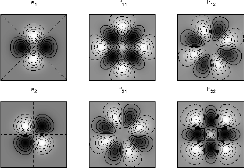
Figure 2: The panels on the left show the pair of functions $w_{1}$, $w_{2}$ with $w_{\alpha}(r)={1\over 2}M_{\alpha lm}w(r)r_{l}r_{m}$ which when multiplied by $f_{s}$ and integrated give the polarization statistic $q_{\alpha}$. The four panels on the right show the components of the polarizability kernel ${\cal P}_{\alpha\beta}(r)$ which when multiplied by $f_{\rm o}$ and integrated yields the polarizability $P_{\alpha\beta}$. The PSF was computed from a turbulence limited OTF $\tilde{g}=\exp(-0.5(kr_{*})^{5/3})$, and the smoothing kernel was $w(r)=\exp(-0.5(r/r_{*})^{2})$ with scale length $r_{*}$ equal to one eighth of the box side.

Equation (42), along with the appropriate expression for $P_{A\beta}(r)$ tells us how the polarization statistic for an individual object formed from weighted quadrupole moments responds to a gravitational shear. This is an essential ingredient in calibrating the shear-polarization relation for a population of galaxies. As we shall see in the next section, there are some subtleties involved, but for now we note that if we simply average (42) over all galaxies on a patch of sky we have

$$\langle q^{\prime}_{\alpha}\rangle-\langle q_{\alpha}\rangle=\langle P_{\alpha\beta}\rangle\gamma_{\beta}$$ (49)

so an estimate of the net shear is given by

$$\hat{\gamma}_{\alpha}=\langle P_{\alpha\beta}\rangle^{-1}(\langle q^{\prime}_{\beta}\rangle-\langle q_{\beta}\rangle)$$ (50)

Which is the generalization of (23) to weighted moments. The term $\langle q^{\prime}_{\beta}\rangle$ in (50) is the averaged observed polarization. The term $\langle q_{\alpha}\rangle$ is the mean polarization generated by anisotropy of the PSF, and we will show how this can be dealt with below.

Ideally, in averaging polarizations, one should apply weight proportional to the square of the signal to noise ratio, which one would expect to be a function of the flux, size, eccentricity etc. of the objects. If the shape is measured with some fairly compact window function $w(r)$, then the total flux, which may be dominated by the profile of the object at considerably larger radius, is probably not ideal and one will likely obtain better performance if one takes the weight function to be a function of $q_{0}$, $q^{2}\equiv q_{\alpha}q_{\alpha}$ and a weighted flux

$$F=\int d^{2}r\;w(r)f_{s}(r).$$ (51)

The response of $F$ can be computed in much the same way as $q_{A}$, and we find from (38) $\delta F=R_{\alpha}\gamma_{\alpha}$ with $R_{\alpha}=\int d^{2}r\;{\cal R}_{\alpha}f_{\rm o}(r)$ with

$${\cal R}_{\alpha}(r)=M_{\alpha ij}[r_{i}(g^{\dagger}\oplus\partial_{j}w)-(r_{i}h)\oplus g^{\dagger}\oplus\partial_{j}w)]$$ (52)

or, for the case $g^{\dagger}=g$,

$${\cal R}_{\alpha}(r)=M_{\alpha ij}[2r_{i}(g\oplus\partial_{j}w)-g\oplus\partial_{j}wr_{i})].$$ (53)

In the foregoing we have implicitly assumed that applying a shear does not affect the location of an object. This is not necessarily the case. If objects are detected as peaks of the surface brightness $f_{\rm o}$ smoothed with some detection filter $w_{d}$, that is as peaks of $f_{d}=w_{d}\otimes f_{\rm o}$, then for an object which in the absence of shear lies at the origin, we have $d_{i}(0)=\partial_{i}(w_{d}\otimes f_{\rm o})_{0}=\int d^{2}r\;\partial_{i}w_{d}(r)f_{\rm o}(r)=0$ while after applying a shear we have $d_{i}(0)=\gamma_{\alpha}M_{\alpha lm}\int d^{2}r\;\partial_{i}w_{d}[r_{l}\partial_{m}f_{\rm o}-(r_{l}\partial_{m}h)\otimes f_{\rm o}]$. This will not, in general, vanish, implying that the peak location will have shifted, and consequently the central second moments should be measured about the shifted peak location, whereas in the above formulae we have computed the change in the moments without taking the shift into account. One could incorporate this effect, but at the expense of considerable complication of the results. There is some reason to think that this effect is rather weak. In particular, if the galaxy is symmetric under rotation by 180 degrees, so $f_{\rm o}(r)=f_{\rm o}(-r)$, then the shift in the centroid vanishes. In general this is not the case, and the formulae above should be considered only an approximation.

3.2 Response of the Population

Equation (50) above gives a properly calibrated estimate of the gravitational shear. It is, however, less than ideal as the polarization average is taken over all galaxies with equal weight. This is neither desirable nor is it achievable in practice due to selection limits, and what one would rather have is an expression for the average induced polarization for all galaxies in some cell of flux, size and shape space, which we parameterize by $F$, $q_{0}$, and $q^{2}\equiv q_{\alpha}q_{\alpha}$. One can then average appropriately weighted combinations of the average shear estimate for each cell. The mean induced polarization for such a cell depends not only on the polarizabilities of the objects contained therein, but also on the gradient of the mean density of objects as a function of the photometric parameters $F$, $q_{0}$, $q_{\alpha}$. Consider a slice through this 4-space at constant $F$, $q_{0}$. A shear will induce a general flow of particles in this space in the direction $\hat{q}_{\alpha}=\hat{\gamma}_{\alpha}$. The mean polarisation for a cell in $F-q_{0}-q^{2}$ is the average around an annulus in $q_{\alpha}$ space, and depends quite sensitively on the local slope of the distribution of particles in $|q_{\alpha}$. These factors can have a profound influence on the weighting scheme; for a distribution which is flat near the origin in $q_{\alpha}$ space, like a Gaussian for example, nearly circular objects have no response and should therefore receive no weight. For a randomly oriented distribution of circular disk galaxies, in contrast, the distribution in $q_{\alpha}$-space has a cusp at the origin; the response becomes asymptotically infinite, and these objects dominate the optimally weighted combination. These examples are both idealized, but underline the importance of computing the population response in order to obtain optimal signal to noise.

Let us first compute the conditional mean polarization for galaxies of a given flux and size: $\langle q_{\alpha}\rangle_{F,q_{0}}$. The mapping of the photometric parameters $F$, $q_{0}$, $q_{\alpha}$ is

$$\matrix{F^{\prime}=F+R_{\beta}\gamma_{\beta}\cr q^{\prime}_{0}=q_{0}+P_{0\beta}\gamma_{\beta}\cr q^{\prime}_{\alpha}=q_{\alpha}+P_{\alpha\beta}\gamma_{\beta}}$$ (54)

so we need to consider the distribution of galaxies in $F,\;q_{0},\;q_{\alpha},\;R_{\alpha},\;P_{0\alpha},\;P_{\alpha\beta}$ with lensed and unlensed distribution functions related by

$$n^{\prime}(F^{\prime},q^{\prime}_{0},q^{\prime}_{\alpha},R^{\prime}_{\alpha},P^{\prime}_{0\alpha},P^{\prime}_{\alpha\beta})dF^{\prime}dq^{\prime}_{0}d^{2}q^{\prime}d^{2}Rd^{2}P^{\prime}_{0}d^{4}P^{\prime}=n(F,q_{0},q_{\alpha},R_{\alpha},P_{0\alpha},P_{\alpha\beta})dFdq_{0}d^{2}qd^{2}Rd^{2}P_{0}d^{4}P.$$ (55)

Multiplying by $W(F^{\prime},q^{\prime}_{0})q^{\prime}_{\alpha}$, where $W$ is some arbitrary function, and integrating over all variables we have

$$\int dF^{\prime}dq^{\prime}_{0}d^{2}q^{\prime}d^{2}Rd^{2}P^{\prime}_{0}d^{4}P^{\prime}n^{\prime}W(F^{\prime},q^{\prime}_{0})q^{\prime}_{\alpha}=\int dFdq_{0}d^{2}qd^{2}Rd^{2}P_{0}d^{4}PnW(F+\delta F,q_{0}+\delta q_{0})(q_{\alpha}+\delta q_{\alpha}).$$ (56)

Now to zeroth order in $\gamma$ this vanishes because of statistical anisotropy of the unlensed population, so using (54) for $\delta F$ etc. and performing a Taylor expansion of $W(F+\delta F,q_{0}+\delta q_{0})$ and integrating by parts we have

$$\int dF^{\prime}\ldots d^{4}P^{\prime}\;n^{\prime}W(F^{\prime},q^{\prime}_{0})q^{\prime}_{\alpha}=\gamma_{\beta}\int dF\ldots d^{4}P\;W(q_{0})\left(nP_{\alpha\beta}-P_{0\beta}q_{\alpha}{\partial n\over\partial q_{0}}-R_{\beta}q_{\alpha}{\partial n\over\partial F}\right).$$ (57)

To first order in $\gamma$ we can replace unprimed by primed quantities throughout the integral on the RHS since we need to compute this only to zeroth order accuracy. We now have a relation between the mean value of the observed polarization on the LHS and some other observable, again integrated over the distribution of observed galaxy properties (rather than of the unlensed parent distribution). Since $W(q_{0})$ is arbitrary, and dropping primes, this implies

$$\int d^{2}qd^{2}Rd^{2}P_{0}d^{4}Pnq_{\alpha}=\gamma_{\beta}\int\cdots\int d^{2}qd^{2}Rd^{2}P_{0}d^{4}P\left(nP_{\alpha\beta}-P_{0\beta}q_{\alpha}{\partial n\over\partial q_{0}}-R_{\beta}q_{\alpha}{\partial n\over\partial F}\right)$$ (58)

or equivalently, that the conditional average polarization is

$$\langle q_{\alpha}\rangle_{F,q_{0}}=\gamma_{\beta}\left[\langle P_{\alpha\beta}\rangle-{1\over n}{\partial n\langle P_{0\beta}q_{\alpha}\rangle\over\partial q_{0}}-{1\over n}{\partial n\langle R_{\beta}q_{\alpha}\rangle\over\partial F}\right]_{F,q_{0}}$$ (59)

where $n=n(F,q_{0})$. Thus, as expected, the shear induced shift in the mean polarization for galaxies of a given size and flux differs from the mean of the shift $\delta q_{\alpha}=P_{\alpha\beta}\gamma_{\beta}$ for an individual object. This is because a shear changes the weighted flux and size of an object in a way which is correlated with its shape. When we average the shear for galaxies in some cell in flux-size space we are averaging over galaxies which have been scattered in size and flux and we obtain a bias in the net polarization which depends on the gradients of the distribution function.

We can generalize this to compute the response for galaxies of given flux $F$, size $q_{0}$, and rotationally invariant shape parameter $q^{2}=q_{\alpha}q_{\alpha}$. To do this, we set $q_{\alpha}=q\hat{q}_{\alpha}$ with the unit polarization vector $\hat{q}_{\alpha}=\{\cos\varphi,\sin\varphi\}$, so $d^{2}q=qdqd\varphi$. We then have, now for some arbitrary function $W(F,q_{0},q^{2})$,

$$\int dF^{\prime}dq^{\prime}_{0}d{q^{2}}^{\prime}d\varphi^{\prime}d^{2}Rd^{2}P^{\prime}_{0}d^{4}P^{\prime}n^{\prime}W(F^{\prime},q^{\prime}_{0},{q^{2}}^{\prime})q^{\prime}_{\alpha}=\int dFdq_{0}dq^{2}d\varphi d^{2}Rd^{2}P_{0}d^{4}PnW(F+\delta F,q_{0}+\delta q_{0},q^{2}+\delta q^{2})(q_{\alpha}+\delta q_{\alpha})$$ (60)

where now $n=n(F,q_{0},q^{2},\varphi,R_{\alpha},P_{0\alpha},P_{\alpha\beta})$. Using $\delta F$ etc. from (54) and $\delta q^{2}=2q_{\eta}P_{\eta\beta}\gamma_{\beta}$ we have

$$\int d\varphi d^{2}Rd^{2}P_{0}d^{4}Pnq_{\alpha}=\gamma_{\beta}\int d\varphi d^{2}Rd^{2}P_{0}d^{4}P(nP_{\alpha\beta}-R_{\beta}q_{\alpha}\partial n/\partial F-P_{0\beta}q_{\alpha}\partial n/\partial q_{0}-2P_{\eta\beta}\partial nq_{\eta}q_{\alpha}/\partial q^{2})$$ (61)

or equivalently $\langle q_{\alpha}\rangle_{F,q_{0},q^{2}}={\overline{P}}_{\alpha\beta}\gamma_{\beta}$ with effective polarizability

$${\overline{P}}_{\alpha\beta}=\langle P_{\alpha\beta}\rangle-{2\over n}{\partial n\langle q_{\eta}P_{\eta\beta}q_{\alpha}\rangle\over\partial q^{2}}-{1\over n}{\partial n\langle P_{0\beta}q_{\alpha}\rangle\over\partial q_{0}}-{1\over n}{\partial n\langle R_{\beta}q_{\alpha}\rangle\over\partial F}$$ (62)

where now $n=n(F,q_{0},q^{2})$, and all averages are at fixed $F,\;q_{0},\;q^{2}$.

The photometric parameters $q_{0},q_{\alpha}$ appearing here are unnormalized. This is convenient for computing the linear response functions. It is, however, somewhat awkward here since the distribution function $n(F,q_{0},q^{2})$ is highly skewed since $q_{0}$ and $q^{2}$ correlate very strongly with the flux. In computing the effective polarizability it is more convenient to work with rescaled variables $q_{0}^{\prime}=q_{0}/F$, and ${q^{2}}^{\prime}=q^{2}/F^{2}$. The distribution function in rescaled variables is

$$n^{\prime}(F,q_{0}^{\prime},{q^{2}}^{\prime})=F^{3}n(F,q_{0},q^{2}).$$ (63)

If we also re-scale the polarizabilities $R_{\alpha}^{\prime}=R_{\alpha}/F$, $P_{A\beta}^{\prime}=P_{A\beta}/F$, ${\overline{P}}_{A\beta}^{\prime}={\overline{P}}_{A\beta}/F$, re-express (62) entirely in terms of primed quantities and then drop the primes we find

$${\overline{P}}_{\alpha\beta}=\langle P_{\alpha\beta}\rangle-{2\over n}{\partial n\langle q_{\eta}P_{\eta\beta}q_{\alpha}\rangle\over\partial q^{2}}-{1\over n}{\partial n\langle P_{0\beta}q_{\alpha}\rangle\over\partial q_{0}}+{1\over n}\left[1-{\partial\over\partial\ln F}+{\partial\over\partial\ln q_{0}}+2{\partial\over\partial\ln q^{2}}\right]n\langle R_{\beta}q_{\alpha}\rangle$$ (64)

where we have used the result that for any function $X(F,q_{0}^{\prime},{q^{2}}^{\prime})$ the partial derivative WRT $F$ at constant $q_{0}$, $q^{2}$ is $(\partial X(F,q_{0}^{\prime},{q^{2}}^{\prime})/\partial F)_{q_{0},q^{2}}=\partial X/\partial F-(q_{0}^{\prime}/F)\partial X/\partial q_{0}^{\prime}-(2{q^{2}}^{\prime}/F)\partial X/\partial{q^{2}}^{\prime}$ to compute the term involving $R_{\alpha}$. The rather cumbersome expression (64) calibrates the relation between the shear and the mean polarization for galaxies in a small cell in flux-size-shape space. To compute it we need to bin galaxies in this space to obtain the mean density $n$ and the various averages appearing here, and then perform the indicated partial differentiation. The form (64) is somewhat inconvenient as the density $n(F,q_{0},q^{2})$ is asymptotically constant as $q^{2}\rightarrow 0$ and one has to properly deal with the discontinuous derivative at this boundary. A computationally more convenient approach is to make one final transformation from $q^{2}\rightarrow q$; since $n(F,q_{0},q)=2qn(F,q_{0},q^{2})$ falls to zero as $q\rightarrow 0$, and there is then no need for any special treatment of the derivatives at the boundary. With this transformation we have

$${\overline{P}}_{\alpha\beta}=\langle P_{\alpha\beta}\rangle-{1\over n}{\partial n\langle q_{\eta}P_{\eta\beta}\hat{q}_{\alpha}\rangle\over\partial q}-{1\over n}{\partial n\langle P_{0\beta}q_{\alpha}\rangle\over\partial q_{0}}+{q\over n}\left[1-{\partial\over\partial\ln F}+{\partial\over\partial\ln q_{0}}+{\partial\over\partial\ln q}\right]n\langle R_{\beta}\hat{q}_{\alpha}\rangle$$ (65)

where now $n=n(F,q_{0},q)$.

What about measurement noise? Let us assume that one has been given an image containing signal and measurement noise, and that one has detected objects, and measured quantities like $F$, $q_{A}$. How would these photometric parameters change under the influence of a gravitational shear? The answer is given by (54), but with the understanding that $R_{\beta}$, $P_{0\beta}$ etc. be the response functions one would measure in the absence of noise. This means that (65) is also applicable with the same proviso. The major terms in (65) are however invariant of additive noise. The exceptions are the terms invoving $\langle P_{0\beta}q_{\alpha}\rangle$ and $\langle R_{\beta}q_{\alpha}\rangle$ which are quadratic in the sky surface brightness. The measured expectation values $\langle P_{0\beta}q_{\alpha}\rangle$ etc. therefore exceed the true values, but by an amount one can calculate from the known properties of the measurement noise. Another implicit assumption in the above analysis is that the objects are actually detected, which restricts applicability to objects which are detected at a reasonable level of significance. Aside from this, the results above should be applicable in the presence of measurement noise. To test these claims we have made extensive simulations with mock data, the details of which are described in appendix B. Figure 3 shows the results of one of these. The actual polarization agrees quite closely with the effective polarizability, even for very faint objects. While the differences between the effective polarizability and that for individual objects is not very large - typically on the order of 20% or so - the effective polarizability clearly describes the true response more faithfully. We shall now use (65) to construct a minimum variance weighting scheme for combining shear estimates.

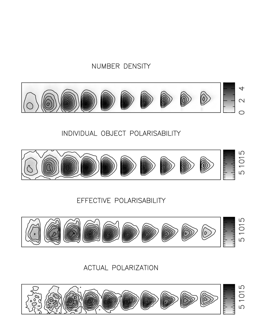
Figure 3: The top panel shows the density of galaxies detected in the simulations described in appendix B as a function of $F$, $q_{0}$, $|q|$. Each of the sub-plots shows the density at fixed $F$ with abscissa $|q|$ and ordinate $q_{0}$. These sub plots are arranged with flux increasing from left to right with flux $F$ increasing by a factor 1.43 at each step. All particles detected with significance level greater than 4-sigma are shown. The panel below this shows the density of particles weighted by the individual object polarizability, and the panel below that shows the density weighted by the effective polarizability given by (65). The lower plot shows the density of objects weighted by the actual polarization (divided by the shear applied in the simulation, or $\gamma=0.1$ in this case).

3.3 Optimal Weighting with Flux, Size and Shape

Armed with the conditional mean polarization $\langle q_{\alpha}\rangle_{F,q_{0},q^{2}}$ we can now compute an optimal weight (as a function of, for example, flux $F$, size $q_{0}$, and eccentricity $q^{2})$ for combining the estimates of the shear from galaxies of different types. Let us assume that one has measured fluxes etc. for a very large number of galaxies — from an entire survey say — and that from these data one has determined the mean number density of galaxies $n(F,q_{0},q^{2})$ and also the various conditional averages and gradients that appear in (65). Now consider a relatively small spatial subsample of these galaxies and bin these into cells in $F,q_{0},q^{2}$ space, and for each bin compute the occupation number $N$ and the summed polarization $\sum q_{\alpha}$.

A shear estimator for a cell which happens to have occupation number $N$ is

$$\hat{\gamma}_{\beta}={\overline{P}}^{-1}_{\alpha\beta}\sum q_{\alpha}/N.$$ (66)

To simplify matters, let us neglect for now any anisotropy of the point spread function, in which case we can write ${\overline{P}}_{\alpha\beta}={\overline{P}}\delta_{\alpha\beta}$ where ${\overline{P}}\equiv{\overline{P}}_{\eta\eta}/2$ and we then have

$$\hat{\gamma}_{\beta}={1\over N{\overline{P}}}\sum q_{\beta}.$$ (67)

The expectation value for the variance in $\hat{\gamma}$ (for a cell which happens to contain $N$ galaxies) is

$$\langle\hat{\gamma}^{2}\rangle=\langle\sum q^{2}\rangle/(N^{2}{\overline{P}}^{2})=q^{2}/N{\overline{P}}^{2}$$ (68)

where we have used $\langle(\sum q_{\alpha})(\sum q_{\alpha})\rangle=\langle\sum q^{2}\rangle$ since, in the limit of weak shear, the galaxy polarizations are uncorrelated. As different cells give shear estimates whose fluctuations are mutually uncorrelated, the optimal way to combine the shear estimates from all the cells is to average them with weight per cell $W_{\rm cell}\propto 1/\langle\hat{\gamma}^{2}\rangle=N{\overline{P}}^{2}/q^{2}$ to obtain a final optimized total shear estimate

$$\hat{\gamma}_{\alpha}^{\rm total}={\sum\limits_{\rm cells}(N{\overline{P}}^{2}/q^{2})({1\over N{\overline{P}}}\sum q_{\alpha})\over\sum\limits_{\rm cells}N{\overline{P}}^{2}/q^{2}}={\sum\limits_{\rm galaxies}{\overline{P}}q_{\alpha}/q^{2}\over\sum\limits_{\rm galaxies}{\overline{P}}^{2}/q^{2}}={\sum\limits_{\rm galaxies}Q\hat{q}_{\alpha}\over\sum\limits_{\rm galaxies}Q^{2}}$$ (69)

where $Q\equiv{\overline{P}}/q$. Thus the optimized cell weighting scheme corresponds to averaging the shear estimates from individual galaxies $\hat{\gamma}_{\alpha}^{\rm galaxy}=q_{\alpha}/{\overline{P}}$ (for galaxies of given $F,q_{0},q^{2}$) with weights $W_{\rm galaxy}={\overline{P}}^{2}/q^{2}$.

The variance in the total shear estimator is

$$\langle\gamma^{2}\rangle={\sum Q^{2}\langle\hat{q}^{2}\rangle\over(\sum Q^{2})^{2}}=(\sum Q^{2})^{-1}.$$ (70)

The quantity $\sum Q^{2}$ is extensive with the number of galaxies and its value, per unit solid angle of sky, provides a useful figure of merit for weak lensing data. From a 2.75hr I-band integrations of solid angle $d\Omega=0.165$ square degrees at CFHT taken in good seeing ($0^{\prime\prime}.60$ FWHM) we obtained $\sum Q^{2}\simeq 4.7\times 10^{4}$ Kaiser et al. (1998) or $\sum Q^{2}/d\Omega\simeq 2.85\times 10^{5}/{\rm sq\;degree}$, so with data of this quality, the statistical uncertainty in the net shear (per component) measured over one square degree would be around $\sigma_{\gamma}\simeq(2\times 2.85\times 10^{5})^{-1/2}=1.32\times 10^{-3}$.

This figure of merit allows one to tune the parameters of one’s shape measurement scheme, such as the weight function scale size, in an unbiased and objective manner. The weighting scheme derived above is appropriate if the shear is independent of the measured flux etc. This is the case for lensing by low redshift clusters where for all relevant values of source redshift the sources are effectively ‘at infinity’ and the shear has saturated at its value for an infinitely distant source $\gamma^{\infty}_{\alpha}$. For high redshift lenses the shear will vary with source redshift, and if one has some, perhaps probabilistic, distance information at one’s disposal, then the weighting scheme should be modified. Let us assume that the measured photometric properties $p_{i}$ of some object indicate it has a probability distribution to be at distance $z$ of $p(z|p_{i})$; with high resolution spectroscopy this would be a delta-function at the measured redshift whereas with only broadband colors the conditional probability would be smeared out and perhaps multimodal. The conditional mean shear for this object, for a given a foreground lens, is proportional to the mean inverse critical critical surface density, and the optimal estimate for the shear at infinity is

$$\hat{\gamma}_{\beta}^{\infty}={1\over\Sigma_{\rm crit}(\infty)}{\sum\limits_{\rm galaxies}\langle 1/\Sigma_{\rm crit}(z)\rangle Qq_{\alpha}\over\sum\limits_{\rm galaxies}\langle 1/\Sigma_{\rm crit}(z)\rangle^{2}Q^{2}}$$ (71)

4 Correction for PSF Anisotropy

In the foregoing we have computed how the shape polarization $q_{\alpha}$ responds to a shear. This allows us to correctly calibrate the circularizing effect of seeing. In general, asymmetry of the PSF will also introduce spurious systematic shape polarization $\langle q_{\alpha}\rangle$ in (50), and it is crucial that this be measured and corrected for. As discussed in §1, for unweighted second moments, the effect of PSF anisotropy is rather simple since the (flux normalized) final second moment $q_{lm}$ is the sum of the intrinsic second moment and that of the instrument, so the anisotropic parts of the instrumental second moment $q_{\alpha}=M_{\alpha lm}q_{lm}$ can be measured from stars, and subtracted from those observed. For weighted or isophotal moments things are more complicated, and depend on how the anisotropy is generated. KSB considered a simple model in which the final PSF is the convolution of some circularly symmetric PSF with a small, but highly asymmetric ‘anisotropizing kernel’ $k(r)$. In §4.1 we will further explore this ‘convolution model’, the attempts that have been made to implement this perturbative approach, and estimate the error in this method. In §4.2 we show that the convolution model is quite inappropriate when applied to diffraction limited seeing and we develop a more general technique for correcting PSF anisotropy. Finally, in §4.3 we draw attention to a type of noise related bias that affects shear estimators, but which has hitherto been overlooked, and we show how this can be dealt with.

The artificial polarization produced by PSF anisotropy is an effect which is present in the absence of any gravitational shear. Thus at leading order in $\gamma$ we can set $\gamma=0$. This effectively decouples the computation and correction of the PSF anisotropy from the shear-polarization calibration problem considered above. It also means that in this section we can assume that the intrinsic shapes of galaxies are statistically isotropic.

4.1 The Convolution Model

KSB computed the effect of a PSF anisotropy under the assumption that this can be modeled as the convolution of a perfect circular PSF with some compact kernel $k(r)$. This would be a good model, for instance, for observations primarily limited by atmospheric turbulence with seeing disk of radius $r_{g}$, but with very small guiding or registrations errors or optical aberrations with extent $\delta r\ll r_{g}$, and the KSB analysis gives a correction to lowest order in $\delta r$. In this model, the effect of ‘switching on’ the anisotropy is the transformation on the observed image, which is smooth on scale $\sim r_{g}$,

$$f_{\rm o}(r)\rightarrow f_{\rm o}^{\prime}(r)=\int d^{2}r^{\prime}\;k(r^{\prime})f_{\rm o}(r-r^{\prime})=f_{\rm o}(r)-k_{i}\partial_{i}f_{\rm o}(r)+{1\over 2}k_{ij}\partial_{i}\partial_{j}f_{\rm o}(r)-{1\over 6}k_{ijk}\partial_{i}\partial_{j}\partial_{k}f_{\rm o}(r)+\ldots$$ (72)

where we have Taylor expanded $f_{\rm o}(r-r^{\prime})$ and where $k_{i}\equiv\int d^{2}rr_{i}k(r)$, $k_{ij}\equiv\int d^{2}rr_{i}r_{j}k(r)$ etc. Taking the kernel to be centered, we have $k_{i}=0$, and to lowest non-vanishing order the effect on the polarization is

$$q_{\alpha}^{\prime}=\int d^{2}r\;w_{\alpha}(r)f_{\rm o}^{\prime}(r)=q_{\alpha}+{1\over 2}k_{ij}\int d^{2}r\;f_{\rm o}(r)\partial_{i}\partial_{j}w_{\alpha}(r)$$ (73)

where $w_{\alpha}\equiv M_{\alpha lm}w(r)r_{l}r_{m}$ and we have integrated by parts. The induced stellar polarization is linear in $k_{ij}$ and therefore scales as the square of the extent of the convolving kernel since $k_{ij}\sim\delta r^{2}$. Performing the decomposition $k_{ij}=k_{A}M_{Aij}$ we find that an individual galaxy’s polarization $q_{\alpha}$ will depend on both the trace $k_{0}$ and the trace-free parts $k_{\alpha}$ of $k_{ij}$. The average induced polarization, however, only depends on $k_{\alpha}$ and we have $\langle q_{\alpha}\rangle=k_{\beta}P^{\rm sm}_{\alpha\beta}$ with

$$P^{\rm sm}_{\alpha\beta}={1\over 2}M_{\alpha lm}M_{\beta ij}\int d^{2}r\;\langle f_{\rm o}\rangle\partial_{i}\partial_{j}(w(r)r_{l}r_{m}).$$ (74)

To lowest order in the PSF anisotropy we can use the KSB polarizability (74) to infer $k_{\alpha}$ from the shapes of stars, and then correct the weighted second moments or the galaxies. At the same level of precision one can convolve one’s image with a small kernel designed to nullify the anisotropy. ?) have presented a $3\times 3$ smoothing kernel which does this. In the typical situation, the shapes are measured from an average of numerous images taken with a pattern of shifts, and which are co-registered to fractional pixel precision, and a simpler but equally effective approach is then to average over pairs of images which have been deliberately displaced from the true solution by the small displacement vector $\pm\delta r=\sqrt{|k_{A}|}\{\cos(\theta),\sin(\theta)\}$ with $\theta=\tan^{-1}(k_{2}/k_{1})/2+\pi/2$.

What is the error in this linearized approximation? To answer this we must consider higher terms in the expansion (72). The next order correction to $q_{\alpha}$ involves $k_{ijk}$ which, unlike the centroid $k_{i}$ cannot be set to zero, so for a given object the fractional error in the KSB correction is on the order of $\delta r/r_{0}\sim\sqrt{e_{\alpha}}$. Galaxies, however, are randomly oriented on the sky, so the average change in $q_{\alpha}$ for a galaxy of some arbitrary morphology but averaged over all position angles at this order in $\delta r/r_{0}$ is

$$\langle\delta q_{\alpha}\rangle\sim k_{ijk}\int d^{2}r\;\langle f_{\rm o}(r)\rangle\partial_{i}\partial_{j}\partial_{k}w_{\alpha}(r).$$ (75)

This vanishes since $\langle f_{\rm o}(r)\rangle$ is an even function while $\partial_{i}\partial_{j}\partial_{k}w_{\alpha}(r)$ is odd, provided we take $w(r)$ to be circularly symmetric at least, which we will assume is the case. The effective net fractional error in the KSB approximation is therefore on the order of $(\delta r/r_{0})^{2}$, or typically on the order of the induced stellar ellipticity.

4.2 General PSF Anisotropy Correction

In principle, one can develop a higher order correction scheme within the context of this model, but this does not seem to be particularly promising; it is not clear that the result will be sufficiently robust and accurate for even for ground based observations — in very good seeing conditions the PSF anisotropy from aberrations becomes large, and the perturbative approach will break down. Moreover, for observations with telescopes in space, the model of the PSF as a convolution of a perfect circular PSF with a kernel, small or otherwise, is wholly unfounded. The instantaneous OTF is

$$\tilde{g}(k)=\int d^{2}r\;A(r)A(r+kD\lambda/2\pi)\exp(i[\varphi(r)-\varphi(r+kD\lambda/2\pi)])$$ (76)

where $A$ is the real transmission function of the telescope input pupil, $D$ is the focal length, and $\varphi(r)$ is the phase error due to mirror aberrations and the atmosphere. It is often said that the general OTF factorizes into a set of terms describing the atmosphere; the telescope aperture; and aberrations, and this would seem to justify the convolution model discussed above. For atmospheric turbulence, and for aberrations arising from random small scale mirror roughness this is correct. This is because the average of the complex exponential term in (76) depends only on $\delta r=kD\lambda/2\pi$ and is independent of $r$, and (76) then factorizes into two independent terms, and the PSF is then the convolution of two completely independent and non-negative functions, but this is not the case in general. To be sure, one can write the combined aperture and aberration OTF as a product of some ‘perfect’ OTF with some other function (the true OTF divided by the perfect one) but quite unlike the case for random turbulence and mirror roughness, this function is neither independent of the shape of the pupil, nor is it positive; if you compute this function for a telescope subject to a low order aberration from figure error, for instance, you will find that the this function is strongly oscillating and is just as extended as the true PSF. Consider the situation in WFPC2 observations, for example, where the PSF anisotropy has important contributions from both from asymmetry of the pupil $A(r)$ and from phase errors, though with the former tending to dominate (though not enormously so) for long wavelengths and far off axis with the WFPC2. The aperture function for the lower left corner of chip 2 computed from the Tiny-Tim model Krist (1995) is shown in figure 4. The off-axis pupil function is approximately that on-axis minus a disk of some radius $r_{1}$ at some distance $\Delta r$ off-axis. If we let the radius of the primary be $r_{0}$ and define a disk function $D_{r_{0}}(r)=\Theta(r/r_{0}-1)$ then on computing the electric field amplitude $a(x)$ and squaring we find that the on-axis PSF is of course given by the Airy disk: $g\simeq\tilde{D}_{r_{0}}^{2}$ while the off axis PSF $g^{\prime}$ is given by $g^{\prime}(x)\simeq g(x)-\tilde{D}_{r_{1}}\tilde{D}_{r_{0}}\cos(2\pi x\Delta r/D\lambda)$. For $r_{1}\ll r_{0}$, $\tilde{D}_{r_{1}}$ is relatively slowly varying and close to unity, in which case the extra off-axis obscuration introduces a perturbation which is proportional to the product of $D_{0}$ and a planar wave, or essentially an asymmetric modulation of the side lobes of the on-axis PSF (see LH panel of figure 5).

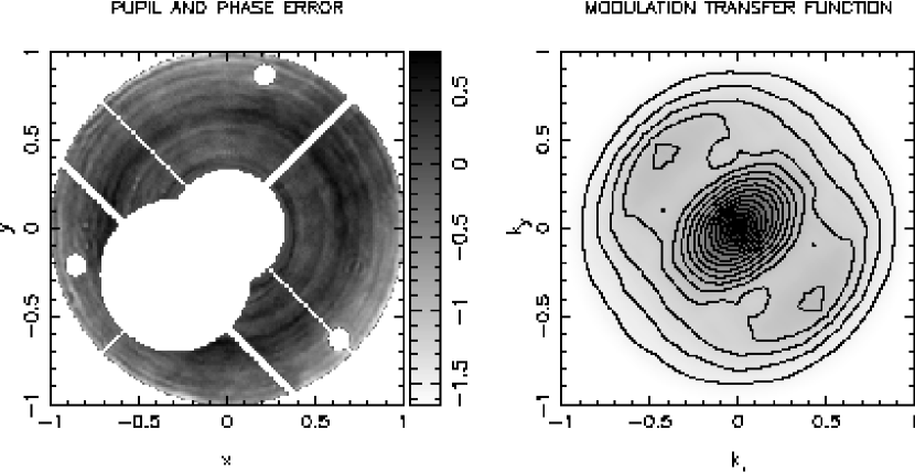
Figure 4: The panel on left shows the WFPC2 pupil function and phase error from Krist’s Tiny Tim model for an off-axis point on the focal plane. The phase is given in radians for a wavelength of 800 nm. The panel on the right shows the modulation transfer function (the real part of the OTF).

In general then, and especially for diffraction limited observations, the perturbative convolution model cannot be trusted. Luckily, at least in the context of the shear estimators discussed here, a simple solution clearly presents itself: Since to compute the polarizability requires that one generate a rather detailed model of the PSF, and that we probably want to apply some kind of re-convolution $f_{\rm o}\rightarrow f_{s}=g^{\dagger}\otimes f_{\rm o}$ to obtain a well behaved shear response, we might as well use the opportunity to choose $g^{\dagger}(r)$ in order to re-circularize the PSF exactly. For example, from the observed PSF, one can compute the OTF $\tilde{g}(k)$ and then form the circularly symmetric function $\tilde{g}_{\rm min}(k)$ being the greatest real function which lies everywhere below $|\tilde{g}(k)|$. The function $g^{\dagger}(r)$ with transform

$$\tilde{g}^{\dagger}(k)=\tilde{g}_{\rm min}(k)^{2}/\tilde{g}(k)$$ (77)

both guarantees a well defined shear polarizability and gives a perfectly circular resulting total PSF. This is illustrated in figure 5.

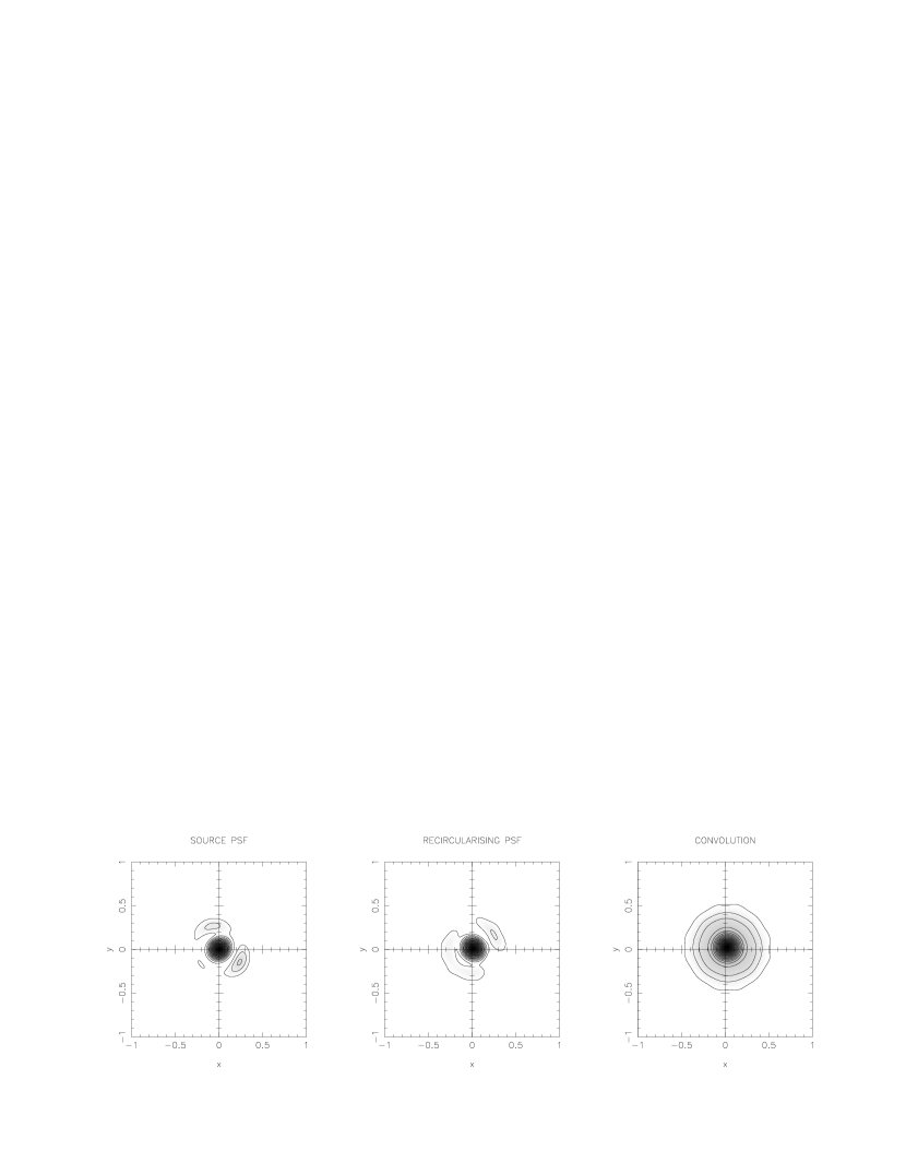
Figure 5: HST WFPC2 PSF from Tiny Tim and re-circularizing filter computed as described in the text.

In some situations the PSF may have near 180 degree symmetry, in which case a good approximation is to re-convolve with a PSF which has been rotated through 90 degrees. Since the PSF is real, the OTF must satisfy the symmetry $\tilde{g}(k)=\tilde{g}^{*}(-k)$. In the absence of aberrations, a diffraction limited telescope has OTF $\tilde{g}=A\oplus A$ which is real and so has exact symmetry under rotation by $\pi$, a property which is shared the PSF, so $R_{\pi}g=g$. If one convolves with $g^{\dagger}=R_{\pi/2}g$ then the resulting total PSF $g^{\dagger}\otimes g$ is symmetric under 90 degree rotations (proof: $R_{\pi/2}\tilde{g}_{\rm tot}=R_{\pi/2}(R_{\pi/2}\tilde{g}\tilde{g})=R_{\pi}\tilde{g}R_{\pi/2}\tilde{g}=\tilde{g}R_{\pi/2}\tilde{g}=\tilde{g}_{\rm tot}$). For a galaxy of given form, the average PSF induced polarization is

$$\langle q_{\alpha}\rangle=\int d^{2}r\;\langle g_{\rm tot}\otimes f\rangle w_{\alpha}=[\langle g_{\rm tot}\otimes f\rangle\otimes w_{\alpha}]_{r=0}=\int{d^{2}k\over(2\pi)^{2}}\langle\tilde{f}\rangle\tilde{g}_{\rm tot}\tilde{w}_{\alpha}$$ (78)

where $w_{\alpha}=M_{\alpha lm}w(r)r_{l}r_{m}$. But $\langle\tilde{f}\rangle$ is circularly symmetric and $\tilde{w}_{\alpha}$ is anti-symmetric under 90 degree rotations, so $\langle q_{\alpha}\rangle=0$. Other situations where this would work would be ground based observations but with large amplitude telescope oscillations, and in fast guiding. In general, however, aberrations from figure errors will introduce both real and imaginary contributions to the OTF and the latter will destroy the exact 180 degree symmetry of the PSF. This is certainly the case for the WFPC2 PSF at optical wavelengths.

In the linearized approximate schemes described earlier, the PSF anisotropy is entirely characterized by the two coefficients $k_{\alpha}$. In general, these will vary substantially with position on the image, but this can be treated by modeling $k_{\alpha}$ as some smoothly varying function of image position $R$ such as a low order polynomial. In the scheme proposed here we need to be able to generate not just these two coefficients, but the full two dimensional PSF $g(r,R)$ (being the intensity at distance $r$ from the centroid of a star at position $R$). A simple practical approach is to solve for a model $g(r,R)=\sum_{I}g_{I}(r)f_{I}(R)$, with $f_{I}(R)$ being some set of polynomial or other basis functions. A least squares fit for the image valued mode coefficients is $g_{I}(r)=m_{IJ}^{-1}G_{J}(r)$ with $m_{IJ}=\sum_{\rm stars}f_{I}(R)f_{J}(R)$; $G_{I}(r)=\sum_{\rm stars}f_{I}(R)g_{\rm obs}(r)$. Armed with the image valued coefficients one can then, for example, compute the convolution $f_{s}=g\otimes f_{\rm o}$ as $f_{s}(r)=\sum_{I}f_{I}(r)(g_{I}\otimes f_{\rm o})$, that is we convolve the source image with each of components $g_{I}(r)$ and then combine with spatially varying coefficients $f_{I}(R)$. Non-linear functions of the PSF such as the re-circularizing kernel $g^{\dagger}$ are easily generated by making realizations of the PSF models on say a coarse grid of points covering the source image, and from each of these computing the desired function, and then fitting the results to a low order polynomial just as for $g(r,R)$.

The approach described here lends itself very nicely to observations with large mosaic CCD cameras, in which misalignment of the chip surfaces and the focal plane coupled with telescope aberrations can give rise to a PSF which varies smoothly across each chip, but which changes discontinuously across the chip boundaries. This results in a very complicated PSF pattern on the final image obtained by averaging over many dithered images. It is a good deal simpler to re-circularize each of the contributing images. We still need to generate a spatially varying model of the final $g(r)$, $g^{\dagger}(r)$ in order to compute the polarizability, but if we fail to model these exactly, it will only introduce a relatively minor error in the shear-polarization calibration.

4.3 Noise Bias

In the absence of noise, the recircularization procedure exactly annuls any PSF anisotropy; the signal content of the image is exactly statistically isotropic. The noise component in the images (which in the original images is incoherent Poisson noise) will however be correlated with an anisotropic two-point function – the peaks and troughs of the noise will appear as ellipses with correlated position angles. For a given object, the noise is equally likely to produce a positive or negative fluctuation in the polarization $q_{\alpha}$, and the effects cancel out on average. Due to the nature of faint galaxy counts, however, objects of a given observed flux are more likely to be intrinsically fainter objects which have been scattered upward in flux than intrinsically brighter objects which have been scattered down, and there will therefore be a tendency for faint objects to be aligned like the re-circularizing PSF; i.e. oriented opposite to the PSF. We will refer to this as ‘noise-bias’. It should noted that an analogous effect is present in the old KSB anisotropy correction scheme. In that case the noise is isotropic, but objects are detected as peaks of a smoothed image and there is then a tendency for the galaxies close to the threshold for detection to be aligned like the PSF. In the context of perturbative schemes as described in §4.1 there are other unevaluated errors in the correction which are typically of similar order to the noise bias effect, which goes some way to explain why it has been ignored in the past. In the improved PSF anisotropy correction method proposed here it is the leading source of error and it behooves us to analyze and correct for it.

Noise will affect the photometric parameters like $q_{\alpha}$ in two ways; in addition to a straightforward additive noise term, noise will also affect the object detection, and will shift the centroid about which we measure the centered second moments, for instance. In fact, the de-centering effect is quite weak. To see why, consider the following simple (though actually quite practical and realistic) model for the detection and measurement process in which we take the re-circularized image $f_{s}$ and define objects as peaks of the field $F(r)=w\oplus f_{s}$ where $w$ is a some smooth, circularly symmetric weight function (we typically use a compensated ‘Mexican hat’ filter), and the object moments $q_{A}$ are the value of the field $q_{A}(r)=w_{A}\oplus f_{s}$ evaluated at the peak location. Let us assume that there exists some object which, in the absence of noise, would lie at the origin, so for this object we would have

$$\matrix{F=F(0)=\int d^{2}r\;w(r)f_{s}(r)\cr 0=d_{i}(0)=\int d^{2}r\;(\partial_{i}w)f_{s}(r)\cr q_{A}=q_{A}(0)=\int d^{2}r\;w_{A}(r)f_{s}(r)}$$ (79)

where the condition that the object be a peak of $F$ is expressed as the vanishing of the dipole-like quantity $d_{i}(r)=\partial_{i}F$. If we now add noise, and let $f_{s}\rightarrow f_{s}+f_{n}$, where $f_{n}(r)$ is the noise component of the re-circularized image, all of the photometric fields $F(r)$, $d_{i}(r)$, $q_{A}(r)$ will change to $F^{\prime}=F+\delta F=F+w\oplus f_{n}$ etc. The dipole $d_{i}$ will no longer vanish at the origin, but will have some value $d_{i}(0)=\int d^{2}r\;(\partial_{i}w)f_{n}$, and the peak of $F(r)$ will have moved to some position $r_{\rm pk}\neq 0$. In the vicinity of the peak we have $d_{i}(r)\simeq 0+(r-r_{\rm pk})_{j}\times\partial_{j}d_{i}(r)$ and hence, to first order in the noise amplitude, the peak location is

$$r_{i,\rm pk}=-(\partial_{j}d_{i})^{-1}\delta d_{j}=-\left[\int d^{2}r\;\partial_{i}\partial_{j}wf_{s}\right]^{-1}\int d^{2}r\;\partial_{j}wf_{n}$$ (80)

The shift of the peak has no effect on $F$ at first order (because $F$ is stationary) but is does affect the central moments $q_{A}$ and we have

$$\matrix{\delta F=\int d^{2}r\;w(r)f_{n}(r)\cr\delta q_{A}=\int d^{2}r\left[w_{A}(r)-v_{Aj}\partial_{j}w\right]f_{n}}$$ (81)

where

$$v_{Ai}=\left[\int d^{2}r\;(\partial_{i}\partial_{j}w)f_{s}\right]^{-1}\int d^{2}r\;(\partial_{i}w_{A})f_{s}$$ (82)

Thus, in general, the first order change in the second moments $q_{A}$ depends not just on the noise and the kernel $w_{A}$, but on the form of the underlying noise-free image $f_{s}$ through the term involving $v_{Aj}$. There is good reason to think that this form dependence is weak for real objects; the function $\partial_{i}w_{A}$ is an odd function, so the extra term vanishes if the galaxy is symmetric under 180 degree rotations. Also, it is hard to see why the presence of this term would cause a systematic polarization; the change in the polarization $\delta q_{A}$ associated with the centroid shift is proportional to the vector $v_{Aj}$ which, being a function of the re-circularised image $f_{s}$ is equally likely to be positive or negative. For each galaxy that, for a given realisation of noise, suffers a certain $\delta q_{A}$ there is a 180 degree rotated clone which has precisely the same weighted flux, polarization etc. (these being even functions) but which suffers a $\delta q_{A}$ of opposite sign. The kind of effect envisioned in the leading paragraph of this sub-section arises if there is a correlation between fluctuations in the polarisation and the flux $F$, coupled with a gradient of the density of objects $n(F)$. The first term in $\delta q_{A}$ in (81) does, as we shall see, indeed correlate with $\delta F$, but, when we average over orientation of the underlying noise-free galaxies, the second does not. Unfortunately, we have not been able to rigorously demonstrate that the centroid shift term vanishes. Nonetheless, in what follows we will assume that this term is negligible. This should certainly be adequate in order to estimate the magnitude of the effect, and is probably sufficiently accurate to give a useful correction, though the results should strictly be regarded as only approximate.

Let us now assume one has measured a set of $n$ photometric parameters $p_{i}$ for a galaxy which, like $F$, $q_{0}$, $q_{\alpha}$, are linear functions of the brightness $f_{\rm o}$ and of the form $p_{i}=\int d^{2}r\;K_{i}(r)f_{\rm o}(r)$. The effect of noise in the images will be to introduce a perturbation in these parameters $\delta p_{i}$. These perturbations have zero mean, $\langle\delta p_{i}\rangle=0$, and since there are typically a very large number of photons (noise plus signal) contributing to the parameters $p_{i}$, the central limit theorem dictates that the $\delta p_{i}$ will have a multivariate Gaussian distribution:

$$\sigma(\delta p)d^{n}\delta p=((2\pi)^{n}|C|)^{-1/2}\exp(-\delta p_{i}C^{-1}_{ij}\delta p_{j}/2)d^{n}\delta p$$ (83)

where the covariance matrix is $C_{ij}=\langle\delta p_{i}\delta p_{j}\rangle$ and is given by

$$C_{ij}=\int d^{2}r\;K_{i}(K_{j}\otimes\xi_{n})$$ (84)

where $\xi_{n}(r)=\langle f_{n}(r^{\prime})f_{n}(r^{\prime}+r)\rangle$ is the 2-point function of the noise $f_{n}(r)$, and which may be computed as described in appendix A.

For objects which are detected at a fairly high level of significance $\nu\gg 1$, the noise will cause a small modification of the underlying distribution function: $n(p)\rightarrow n^{\prime}(p)$, which we can compute in a perturbative manner:

$$n^{\prime}(p)=\int d^{n}\delta p\;n(p-\delta p)\sigma(\delta p)=n(p)-{\partial n\over\partial p_{i}}\langle\delta p_{i}\rangle+{1\over 2}{\partial^{2}n\over\partial p_{i}\partial p_{j}}\langle\delta p_{i}\delta p_{j}\rangle+\ldots$$ (85)

Since $\sigma(p)$ is an even function, all the odd terms in this expansion vanish, and we have $n^{\prime}(p)=n(p)+{1\over 2}C_{ij}\partial^{2}n/\partial p_{i}\partial p_{j}$ at leading order.

Let us specialize now to the $n=4$ dimensional case: $p_{i}=F,q_{0},q_{\alpha}$ and compute the mean polarization for galaxies of given $F$, $q_{0}$ with some weight function $W(q=|q_{\alpha}|)$:

$$\langle q_{\alpha}\rangle_{F,q_{0}}={\int d^{2}q\;W(q)q_{\alpha}n^{\prime}(F,q_{0},q_{\alpha})\over\int d^{2}q\;W(q)n^{\prime}(F,q_{0},q_{\alpha})}\simeq{\int d^{2}q\;W(q)q_{\alpha}\delta n(F,q_{0},q_{\alpha})\over\int d^{2}q\;W(q)n(F,q_{0},q_{\alpha})}$$ (86)

where $\delta n(F,q_{0},q_{\alpha})={1\over 2}C_{ij}\partial^{2}n/\partial p_{i}\partial p_{j}$. Since $q_{\alpha}$ is an odd function and $W(q)$, $n(F,q_{0},q_{\alpha})$ are even, the only terms which contribute to the integral in the numerator are those involving a single derivative with respect to polarization: $\partial^{2}n/\partial F\partial q_{\beta}$ and $\partial^{2}n/\partial q_{0}\partial q_{\beta}$ and, on integrating by parts, we have

$$\langle q_{\alpha}\rangle={-{1\over 2}\int d^{2}q\;\left(\langle\delta F\delta q_{\beta}\rangle{\partial n\over\partial F}+\langle\delta q_{0}\delta q_{\beta}\rangle{\partial n\over\partial q_{0}}\right){\partial W(q)q_{\alpha}\over\partial q_{\beta}}\over\int d^{2}q\;W(q)n(F,q_{0},q_{\alpha})}$$ (87)

Using $\partial(W(q)q_{\alpha})/\partial q_{\beta}=\delta_{\alpha\beta}W(q)+q_{\alpha}\hat{q}_{\beta}dW/dq$, integrating over angle and converting from $n(F,q_{0},q_{\alpha})$ to $n^{\prime}(F,q_{0},q)=2\pi qn(F,q_{0},q_{\alpha})$ and dropping the prime we have

$$\langle q_{\alpha}\rangle={-{1\over 2}\int dq\;\left(\langle\delta F\delta q_{\alpha}\rangle{\partial n\over\partial F}+\langle\delta q_{0}\delta q_{\alpha}\rangle{\partial n\over\partial q_{0}}\right)(W(q)+{1\over 2}qW^{\prime}(q))\over\int dq\;nW(q)}$$ (88)

and letting $W(q)$ become a delta-function to isolate a single value of $q$ we have

$$n\langle q_{\alpha}\rangle=-{1\over 2}\left(\langle\delta F\delta q_{\alpha}\rangle{\partial n\over\partial F}+\langle\delta q_{0}\delta q_{\alpha}\rangle{\partial n\over\partial q_{0}}\right)$$ (89)

Thus, as anticipated, there is a net induced polarization if there is a non-zero correlation between the polarization fluctuation $\delta q_{\alpha}$ and $F$ and/or $q_{0}$, and also significant gradients of the distribution function with respect to $F$ or $q_{0}$.

The effect on the re-scaled polarization of the first term in (89) is $\langle q^{\prime}_{\alpha}\rangle=\langle q_{\alpha}\rangle/F=-({1\over 2}\langle\delta F\delta q_{\alpha}\rangle/F^{2})\partial\ln n/\partial/lnF$ and is second order in the inverse significance: $\langle q^{\prime}_{\alpha}\rangle\propto\nu^{-2}$, where $\nu^{2}=F^{2}/\langle\delta F^{2}\rangle$ and rapidly becomes small for well observed objects. Thus it should be possible to set a sensible limit on the significance of object detection, and, if necessary, use (89) together with (84) for $\langle\delta F\delta q_{\alpha}\rangle$ etc. to correct for this. The error in this linearized approximation is of fourth order in the inverse significance. As a simple illustrative example consider a Gaussian galaxy of scale $r_{G}$, a Gaussian window function $w$ with scale $r_{w}$, and a Gaussian ellipsoid PSF $g=\exp(-(x^{2}/r_{a}^{2}+y^{2}/r_{b}^{2})/2)$ with $r_{a}=r_{g}(1+\epsilon/2)$, $r_{b}=r_{g}(1-\epsilon/2)$. A suitable recircularising kernel is then $g^{\dagger}=\exp(-(x^{2}/r_{b}^{2}+y^{2}/r_{a}^{2})/2)$ and the normalised two point function of the noise is then

$$\xi_{n}(r)={1\over\pi r_{a}r_{b}}e^{-(x^{2}/2r_{b}^{2}+y^{2}/2r_{a}^{2})/2}$$ (90)

The expectation averages are, to first order in $\epsilon$, $\langle\delta F^{2}\rangle=2(r_{w}^{2}+r_{g}^{2})$; $\langle\delta q_{1}\delta F\rangle=r_{w}^{4}(r_{a}^{2}-r_{b}^{2})/(r_{w}^{2}+r_{g}^{2})=2\epsilon r_{w}^{4}r_{g}^{2}/(r_{w}^{2}+r_{g}^{2})$, and so taking only the first term in (89) for simplicity

$$\langle\delta q_{1}^{\prime}\rangle\equiv{\langle\delta q_{1}\rangle\over F}=-{1\over 2}{\partial\ln n\over\partial\ln F}{1\over\nu^{2}}{\langle\delta q_{1}\delta F\rangle\over\langle\delta F^{2}\rangle}\simeq{1\over 2}{\epsilon\over\nu^{2}}r_{w}^{4}r_{g}^{2}/(r_{w}^{2}+r_{g}^{2})$$ (91)

using $\partial\ln n/\partial\ln F\simeq 1$ as observed. A shear of strength $\gamma$ applied to the Gaussian galaxy produces a polarisation

$$\langle\delta q_{1}^{\prime}\rangle=4\gamma r_{w}^{4}r_{G}^{2}/(r_{G}^{2}+r_{w}^{2}+r_{g}^{2})$$ (92)

therefore a PSF anisotropy of strength $\epsilon$ is equivalent to an effective shear

$$\gamma={\epsilon\over 8\nu^{2}}{r_{g}^{2}\over r_{G}^{2}}{(r_{w}^{2}+r_{g}^{2}+r_{G}^{2})^{2}\over(r_{w}^{2}+r_{g}^{2})^{2}}$$ (93)

or, for $r_{w}=r_{G}=\sqrt{2}r_{g}$ say, $\gamma=25\epsilon/144\nu^{2}$, which for $\nu=6$ and PSF asymmetry $\epsilon=0.3$, which is a reasonable value for off-axis points on the CFHT in good seeing, gives a shear of around $1.4\%$. This is a sizable effect, and should therefore be corrected for.

5 Discussion

We have considered the problem of how to estimate weak gravitational shear from observations which have been degraded by atmospheric and/or instrumental effects. Previous analyses of this problem have made simplifying assumptions which render the results inaccurate. A major result of the paper is the finite resolution shear operator (33) which gives the response of an observed image to a gravitational shear applied before smearing with the PSF. This result can be used to properly calibrate the effect of any shear estimator, and is valid for arbitrary PSF, be it turbulence or diffraction limited. We then focused on the application to weighted moment shear estimators. We have computed the response of individual objects to a shear in §3.1, and the response of the population of background galaxies with given photometric properties in §3.2, and from this we have devised an optimal weighting scheme §3.3. In the last section we have considered the correction for PSF anisotropy. While there are still some approximations in the present analysis, we feel that they place the techniques of shear measurement on a much firmer footing than before.

6 Acknowledgements

I wish to acknowledge helpful discussions with Malcolm Northcott, Francois and Claude Roddier, John Tonry, Ger Luppino, Pat Henry, Ken Chambers, Jeff Kuhn and Christ Ftaclas.

Appendix A Properties of Optical Point Spread Functions

Here we shall briefly review and derive some properties of telescope point spread functions which are used above. For more detailed background the reader should consult (Roddier (1981); Beckers (1993)) and references therein. We will highlight the wavelength or color dependence of the various sources of PSF anisotropy, which may be crucially important for weak lensing searches for large-scale structure and galaxy-galaxy lensing.

According to elementary diffraction theory Born & Wolf (1964) the complex electromagnetic field amplitude $a(x)$ due to a distant source at position $x_{\rm phys}$ on the focal plane (we will suppress polarization subscripts for clarity) is given as an integral over the input pupil

$$a(x_{\rm phys})=\int d^{2}r\;A(r)C(r)e^{2\pi ix_{\rm phys}r/L\lambda}$$ (A1)

where $A(r)$ is the ‘pupil function’ describing the aperture transmission, $C(r)$ is the complex electric field amplitude of the incoming wave, $\lambda$ is the wavelength of the radiation and $L$ is the focal length. The field amplitude $C(r)$ will incorporate any random amplitude and phase variations of the incoming wavefronts due to atmospheric turbulence, whereas constant wavefront distortions due to aberrations in the optical elements of the telescope are incorporated as a complex factor in $A$. Thus $a(x)$ is the Fourier transform of $AC$, evaluated at wave-number $k=2\pi ix/D\lambda$. The PSF $g$ is the square of the field amplitude and in rescaled coordinates $x=2\pi x_{\rm phys}/L\lambda$, is

$$g(x)=|a(x)|^{2}=\int{d^{2}z\over(2\pi)^{2}}e^{-ix\cdot z}\tilde{g}(z)$$ (A2)

where the OTF is

$$\tilde{g}(z)=\int d^{2}rC(r)C^{*}(r+z)A(r)A^{*}(r+z).$$ (A3)

For very short ground-based observations the atmospheric rippling is frozen and the PSF consists of speckles. For long exposures we are taking the time average of the OTF and can replace $C(r)C^{*}(r+z)$ by its time average $\langle C(r)C^{*}(r+z)\rangle=\xi_{C}(z)$. This is independent of $r$, so the OTF factorizes into two independent functions

$$\tilde{g}(z)=\xi_{C}(z)\int d^{2}rA(r)A^{*}(r+z)$$ (A4)

and the same is true for random small scale amplitude or phase fluctuations introduced by e.g. random fine scale mirror roughness.

A.1 Atmospheric Turbulence

Ground based observations on large telescopes are usually limited by atmospheric seeing arising from inhomogeneous random turbulence, and it is a good approximation to ignore the finite size of the entrance aperture and set the factor involving $A$ in (A4) to unity. In the ‘near field’ immediately behind the turbulent layer, the effect on the incoming wave is a pure phase shift $C(r)=e^{i\varphi(r)}$ where $\varphi=2\pi id(r)/\lambda$ and $d(r)$ is the vertical displacement of the wavefront due to turbulence. The displacement $d$ is nearly independent of wavelength, so $\varphi(r)\propto 1/\lambda$. At greater depths this phase shift evolves into a combination of amplitude and phase variations, but the 2-point function $\langle C(r)C^{*}(r+z)\rangle$ remains invariant (Fried (1966); Roddier (1981))and the ‘natural seeing’ OTF is

$$\tilde{g}(z)=\langle e^{i(\varphi(r)-\varphi(r+z))}\rangle.$$ (A5)

For steady turbulence and long integrations the central limit theorem guarantees that the phase error $\psi=\varphi(r)-\varphi(r+z)$ will have a Gaussian probability distribution $p(\psi)=(2\pi\langle\psi^{2}\rangle)^{-1/2}\exp(-\psi^{2}/2\langle\psi^{2}\rangle)$ and so the time average of the complex exponential is

$$\langle e^{i\psi}\rangle=\int d\psi\;p(\psi)e^{i\psi}=\exp(-\langle\psi^{2}\rangle/2)=\exp(-S_{\varphi}(r)/2)$$ (A6)

where the ‘phase structure function’ is

$$S_{\varphi}(\Delta r)\equiv\langle(\varphi_{1}-\varphi_{2})^{2}\rangle.$$ (A7)

There are strong theoretical Tatarski (1961) and empirical reasons to believe that on scales much less than some ‘outer scale’ the turbulence will have the Kolmogorov $n=-11/3$ spectrum, for which $S_{d}(r)\propto r^{5/3}$. The structure function for the phase is conventionally written as $S_{\phi}(r)=6.88(r/r_{0})^{5/3}$ where $r_{0}$ is the ‘Fried length’ Fried (1966) being on the order of tens of cm for typical observing conditions (an $r_{0}$ of 20cm gives a FWHM = $0^{\prime\prime}.5$ at $\lambda=550$ nm). The rms phase difference rises with separation as $r^{5/6}$ in the ‘inertial range’ delimited at the upper end by the outer scale, set by the width of the mixing layer, which recent estimates (Avila et al. (1997); Martin et al. (1998)) find to be around $10-20$m and much larger than $r_{0}$. The on-axis OTF computed from stars in deep CFHT imaging agrees quite well with the theoretical expectation. The inertial range is limited at the low end by diffusion, but at scales much smaller than $r_{0}$, so little error is incurred in ignoring this; in real telescopes mirror roughness and other effects modify the OTF at small scales. These effects dominate the PSF at very large radii, but are unimportant for weak lensing observations.

The optical transfer function is $\tilde{g}(k)=\exp(-S_{\phi}(kD\lambda/2\pi)/2)$ and is real and positive. The PSF is the transform of $\exp(-6.88(z/r_{0})^{5.3})$ with width which scales as $R_{\rm FWHM}\propto\lambda^{-1/5}$ which again is found to apply quite well in practice. This very weak dependence on wavelength is a blessing in weak lensing since one uses stars to measure the PSF for the galaxies, yet the stars and the galaxies may have different colors. The atmospheric PSF is expected to be isotropic. At large angles the PSF has profile $g\propto x^{-11/3}$ so the unweighted second moment of the PSF is not well defined. For Kolmogorov turbulence the log of the OTF is just proportional to $k^{5/3}$ and is well defined for all $k$.

A.2 Fast Guiding

According to the Kolmogorov law, the rms wave-front tilt, averaged over scale $r$ varies as $r^{-1/6}$, which suggests that even for telescopes with reasonably large $D/r_{0}$ there may be useful gain in image quality from fast guiding, and experience with HRCAM on CFHT McClure et al. (1989) would seem to support this, though part of the dramatic improvement is likely due to inadequacy of the existing slow guiding system. A technological advance which may have implications for weak lensing is the advent of on-chip fast guiding Tonry et al. (1997) with OTCCD chips. With a mosaic camera composed of such devices it should be possible to obtain partial image compensation over a large angular scale, with one or more guide stars for each ‘isokinetic’ patch.

The theoretical fast guiding PSF was first explored by ?) who argued that the OTF should take the form of the natural seeing or uncompensated OTF times an ‘inverse Gaussian’ $\exp(+\alpha k^{2})$, with scale factor $\alpha$ given in terms of $D$ and $r_{0}$. This is a physically reasonable picture, since it implies that the natural PSF is the convolution of the corrected PSF with a Gaussian to describe the distribution of tilt, but is only an approximate result. Modified forms of the ‘Fried approximation’ have been explored by ?) and ?), and the fast guiding OTF has been simulated by ?).

It can be shown that in the near-field limit the exact fast-guiding OTF is given by

$$\tilde{g}(z)=\int d^{2}r\;A(r)A(r+z)\exp(-\langle\psi(r,z)^{2}\rangle/2)$$ (A8)

where

$$\langle\psi(r,z)^{2}\rangle=S({\bf z})+z_{i}[(W_{i}\otimes S)_{\bf r}-(W_{i}\otimes S)_{{\bf r}+{\bf z}}]-{1\over 2}z_{i}z_{j}\int d^{2}r^{\prime}\;W_{i}({\bf r}^{\prime})(W_{j}\otimes S)_{{\bf r}^{\prime}}$$ (A9)

and where $W_{i}\equiv\partial_{i}A^{2}$. Examples are shown in figure 6. These plots show that the impact of fast guiding on the atmospheric PSF for large telescopes will be rather modest, at least if current, rather low, estimates of the outer scale are correct. Fast guiding may, however, yield dramatic improvements for small ($\sim 1$m diameter) telescopes. How well this would work depends largely on the altitude of the turbulent layer. The isokinetic patch size (over which stars move coherently) is $\sim D/h$ so for $h=10$km and $D=1$, say, this is on the order of $20^{\prime\prime}$, the motion needs to be sampled at a rate $\mathrel{\raise 1.29167pt\hbox{$>$}\mkern-14.0mu\lower 2.58334pt\hbox{$\sim$}}v/D$ reflecting the relatively high wind speed at high altitude, and it may then be difficult to find bright enough guide stars. There are strong indications (Christian & Racine (1985); Tonry et al. (1997); McClure et al. (1991)) that centroid motions are coherent over much larger angular scales than this, indicating that much of the image degradation arises from low-altitude turbulence, and this greatly improves the outlook as one can determine the local motion by averaging a number of stars, and one can afford to sample at a lower rate. A collection of small telescopes equipped with wide angle OTCCD cameras could be a formidable instrument for weak lensing or other projects requiring high resolution imaging over wide fields. Fast guiding, while offerering important resolution gains, will also present its own challenges since one expects the PSF to become sytematically anisotropic depending on location with respect to the guide stars for the reasons described by ?). Also, fast guiding does not cure PSF anisotropies from telescope aberrations.

Figure 6: Optical transfer functions and corresponding PSFs given by equations (A8, A9) for a range of telescope aperture diameters: $1.0$m solid; $1.5$m dash; $2.2$m dot-dash; $3.6$m dotted; $\infty$ dot-dot-dot-dash. A von Karman turbulence spectrum with outer scale of 20m and Fried length $r_{0}=0.2$m were assumed, and the telescope was assumed to be operating at a wavelength $\lambda=550$nm.

A.3 Atmospheric Dispersion

Variation of the refractive index of the atmosphere with wavelength will cause images to be dispersed into spectra, and the consequent elongation of images was estimated by KSB, who pointed out that this could potentially cause problems when using PSF’s of stars to correct the shapes of galaxies, since the elongation depends on the spectrum of the object; an object with a line-like spectrum, or one with a sharp-edged absorption band which falls within the bandpass, will of course be less dispersed than a continuum object. Here we will make this more quantitative.

Weak-shear measurements are usually made on images composed from multiple exposures taken at a range of air masses and which are co-registered using centroids of foreground stars. The astrometric solution obtained using stars of a variety of spectra will be a compromise. Assuming, as is usually the case, that one has many more stars at ones disposal than the number of coefficients of the transformation one is trying to solve for (typically a low order polynomial), then the solution obtained by minimising least squared residuals will be one which correctly maps surface brightness at some wavelength $\lambda_{0}$ determined by the average properties of the foreground stars, but with photons at other wavelengths displaced by an amount proportional to $\lambda-\lambda_{0}$. The sum of a set of $N$ such images is

$$f_{\rm tot}(r,\lambda)=\sum\limits_{I=1}^{N}f(r+\alpha_{I}(\lambda-\lambda_{0}),\lambda)$$ (A10)

where $f(r,\lambda)$ is the image seen at zenith. The 2-vector $\alpha_{Ii}$ has $|\alpha_{I}|=(\Theta_{0}/\lambda_{0})(\partial\ln\Theta/\partial\ln\lambda)\tan z_{I}$, with $z_{I}$ the zenith distance, and $\hat{\alpha}_{I}$ is directed towards the horizon. Tables of the refraction angle $\Theta(\lambda)$ are given by ?). A star with SED $f_{\lambda}$, and therefore with photon distribution function $S(\lambda)d\lambda\propto\lambda f_{\lambda}d\lambda$, gives, in a photon counting system, a response at zenith $f(r,\lambda)=\delta(r)S(\lambda)$, and the summed image of such a star is then

$$f_{\rm tot}(r)=\int d\lambda f_{\rm tot}(r,\lambda)=\sum\limits_{I=1}^{N}\int d\lambda\delta(r-\alpha_{I}(\lambda-\lambda_{0}))S(\lambda)$$ (A11)

The centroid of a star in the image $f_{\rm tot}(r)$ is an average of the centroids that would be obtained from each of the contributing images. Consider the $I$’th image, and rotate the coordinate system so that $\alpha_{I}$ lies along the $x$-axis. The centroid for this component is $\overline{r}_{I}=({\overline{x}}_{I},0)$ with

$${\overline{x}}_{I}={\int dx\int dy\int d\lambda\;x\delta(x-\alpha_{I}(\lambda-\lambda_{0}))\delta(y)S(\lambda)\over\int dx\int dy\int d\lambda\;\delta(x-\alpha_{I}(\lambda-\lambda_{0}))\delta(y)S(\lambda)}={\alpha_{I}\int d\lambda\;(\lambda-\lambda_{0})S(\lambda)\over\int d\lambda\;S(\lambda)}=\alpha_{I}({\overline{\lambda}}-\lambda_{0})$$ (A12)

from which it follows that the $\lambda_{0}$ which minimises $\langle\overline{x}_{I}^{2}\rangle$, being the average over the stars used for registration of the squared displacement, is $\lambda_{0}=\langle\overline{\lambda}\rangle={1\over n_{\rm stars}}\sum\overline{\lambda}$, i.e. simply the average over the registration stars of their mean wavelength. The centroid for the summed image is

$$\overline{r}_{i}=({\overline{\lambda}}-\lambda_{0})\langle\alpha_{i}\rangle_{I}$$ (A13)

where $\langle\alpha_{i}\rangle_{I}\equiv{1\over N}\sum\alpha_{Ii}$. Similarly, the central second moment is

$$p_{ij}={\int d^{2}r\;(r_{i}-\overline{r}_{i})(r_{j}-\overline{r}_{j})f_{\rm tot}(r)\over\int d^{2}rf_{\rm tot}(r)}=\overline{(\lambda-\lambda_{0})^{2}}\langle\alpha_{i}\alpha_{j}\rangle_{I}-(\overline{\lambda}-\lambda_{0})^{2}\langle\alpha_{i}\rangle_{I}\langle\alpha_{j}\rangle_{I}$$ (A14)

Note that since, for any sensible zenith angle, the width of the spectrum is tiny compared to that of the PSF, this unweighted second moment fully characterises the effect of dispersion.

Consider, for illustration, the case of an equatorial field observed with a telescope near the equator, and for a range of zenith angle $|z|<z_{\rm max}$. In this case $\sum\alpha_{I}=0$, so the second term in (A14) vanishes (this is not a particularly unusual special case; for a number of observations spread over a range of zenith angles, one would generally expect the second term here to become relatively small). When we solve for the PSF from the shapes of foreground stars of various types we are effectively averaging over a mix of SED’s appropriate for a low redshift spiral galaxy. The average PSF moment obtained from the stars can, for the equatorial case, then be written as

$$\langle p_{xx}\rangle=(\langle\overline{\lambda^{2}}\rangle-\langle\overline{\lambda}\rangle^{2})\langle\alpha^{2}\rangle_{I}$$ (A15)

where by $\langle\alpha^{2}\rangle_{I}=(\Theta_{0}/\lambda_{0})^{2}(\partial\ln\Theta/\partial\ln\lambda)^{2}{1\over N}\sum_{I}\tan^{2}z_{I}$, and the SED dependent coefficient of $\langle\alpha^{2}\rangle_{I}$ is the mean of the dispersions of the stars plus the dispersion of the means of the stars. For the equatorial case this is the same as the second moment for a single point like object with an SED like the average SED of the registration stars. This is not strictly true in general, but the difference is probably a minor one, and it then follows that if the faint galaxies have SED’s such that their $\overline{(\lambda-\lambda_{0})^{2}}$ differs systematically from that for a low redshift spiral then the PSF correction will be systematically in error. Figure 7 quantifies the importance of this effect, by using redshifted galaxy SED’s of various types from ?). The panel on the left shows the displacement of the centroid of galaxies of the various indicated types as their spectra are red-shifted, and the right hand panel shows the variation of the second moment of the PSF. We find that the I-band second moment is very stable, with peak fluctuations $\delta p_{lm}\sim 300{\rm mas}^{2}$ for these parameters, and with little systematic difference from a low spiral redshift galaxy if we integrate over a range of redshifts. For illustration, if we take the systematic change in polarisation to be say $\delta p_{lm}\sim 100{\rm mas}^{2}$ and a Gaussian profile galaxy, this corresponds to a shear of $\gamma\simeq 1.38\delta p_{lm}/{\rm FWHM}^{2}\simeq 6\times 10^{-4}(0^{\prime\prime}.5/{\rm FWHM})^{2}$. In the V-band the polarisation fluctuations are larger by a factor 2-3, but even then, and even for marginally resolved objects in excellent seeing the effect is at or below the sensitivity for current and near future surveys. The effect scales as $\langle\tan^{2}z\rangle$ however, so observations at $z\gg 1$ should be avoided. This would also become more of an issue with fast guiding, where we can hope to resolve much smaller objects. The effect is also dependent on the details of the system response function; the CFH12K system having a particularly broad I-band response which exacerbates the effect.

Figure 7: Atmospheric dispersion. Left hand panels show the angular displacement due to changes in the SED for galaxies at a range of redshifts. A zenith angle of 45 degrees was assumed, and upper and lower panels show the deflection for the I-band and V-band system response functions for the CFH12K camera. More concretely, the quantity plotted is the mean wavelength $\overline{\lambda}-\lambda_{0}=\int d\lambda\;(\lambda-\lambda_{0})\lambda f_{\lambda}R(\lambda)/\int d\lambda\;\lambda f_{\lambda}R(\lambda)$ where $f_{\lambda}$ is the SED, $R(\lambda)$ the system response, $\lambda_{0}$ was taken to be $820$nm, and $\overline{\lambda}-\lambda_{0}$ was converted to angle as described in the text, and assuming a 4000m observatory altitude. The V-band plot has been limited to $z<1.5$ since the CWW SED’s are limited to proper wavelength $\lambda>200$nm and redshift past the $V$-band at around $z=1.5$. The plots shows that the shifts due to SED variation are typically on the order of $20$mas in the I-band, but somewhat larger in V. The elliptical/S0 SED shows a somewhat greater excursion at high redshift, but this it caused by the SED red-shifting right out of the filter band, so one would not expect to find many such objects in flux limited samples. The panels on the right show how the width of the spectrum, and hence the PSF polarization, varies with redshift and galaxy type. Here the quantity plotted is $\overline{(\lambda-\lambda_{0})^{2}}=\int d\lambda\;(\lambda-\lambda_{0})^{2}\lambda f_{\lambda}R(\lambda)/\int d\lambda\;\lambda f_{\lambda}R(\lambda)$, again converted to angle, here assuming $\langle\tan^{2}z\rangle=1$.

In the foregoing we assumed that the foreground stars used for registration were numerous and well mixed. With a finite number of stars there will be some additional color dependent error in the registration which, if uncorrected, would give rise to artificial field distortion. However, we have found from simulations using the USNOA catalog as the astrometric reference system that this introduces artificial shear at around the $10^{-4}$ level, which is negligibly small for present and near future surveys.

A.4 Aberrations

Aberrations of the optical elements of the telescope can be a significant contribution to the anisotropy of the PSF. These can be analyzed in the same manner as the wavefront deformation due to the atmosphere, but with a couple of distinctive features: First, for low-order ‘classical’ aberrations where the phase error varies smoothly, and for ground based observing conditions, if an aberration is an important factor then it’s contribution to the OTF will be nearly achromatic. This is because if there is a smooth variation of the wavefront error (rather than a Gaussian random field with power at all scales as in atmospheric turbulence) amounting to $N\gg 1$ wavelengths, then the PSF will be very well approximated by its geometric optics limit with shape defined by the pattern of caustics (though for a narrow band filter, the PSF would actually be found on close examination to be composed of a set of speckle sized patches concentrated along the lines where the classical caustics form Berry & Upstill (1980)). The wavefront deformation can be measured directly from out of focus images Roddier & Roddier (1993) so this contribution to the PSF can be directly predicted.

A.5 Diffraction Limited Seeing

Truly diffraction limited seeing arises when the rms phase error across the aperture (due to the atmosphere and/or aberration of the optical elements of the telescope) is much less than unity. In this case the optical transfer function $\tilde{g}(k)$ is, to a good approximation, just the auto-correlation of the aperture $A\oplus A$ at lag $\Delta r=kD\lambda/2\pi$, and must therefore vanish for spatial frequencies $k>2\pi/(f\lambda)$, where $f$ is the ratio of the aperture diameter to the focal length. The log of the OTF becomes ill defined as one approaches the diffraction limit. From (A4) we see that this cut-off is also present in the case of turbulence dominated seeing, but it occurs at a high frequency where the the optical transfer function has already become exponentially small due to atmospheric effects, and has little impact.

In the absence of aberrations, the OTF for diffraction limited seeing is real and non-negative. The OTF is symmetric under rotations of 180 degrees, and so any quadrupole anisotropy of the PSF can be anulled simply by re-convolving one’s image with a 90 degree rotated PSF. For diffraction limited seeing the size of the PSF scales as the inverse of the wavelength, a fact which can be incorporated in empirical or theoretical Krist (1995) modeling of the PSF.

In the HST WFPC2, figure errors are not negligible. The imaginary part of the OTF is excited to the degree that re-convolution with a 90-degree PSF still leaves non-negligible PSF anisotropy. The phase errors are not large — the telescope is nearly diffraction limited — so this means that the wavelength dependence could be quite complicated. The systematic error arising from differences between faint galaxy and foreground star SED’s can be estimated much as we did for atmospheric dispersion.

A.6 Guiding Errors, Pixellisation, and Detector Effects

So far we have considered the continuous distribution of intensity on the focal plane $f_{\rm o}(r)$. In real detectors we sample the image with a grid of pixels. The response of a pixel in not uniform and has been directly measured for front-illuminated EEV devices by scanning a small spot of light across the CCD (Jorden et al. (1993), Jorden et al. (1994)). They found very little ‘leakage’ of electrons across pixel boundaries, but according to the ?) this is a substantial effect for the WFPC2 instrument on HST; a photon landing in one pixel has a non-negligible probability of being detected by a neighboring pixel instead. Such effects are expected, and found, to depend on wavelength. The value of a pixel is a sample of the convolution of the sky surface brightness with the ‘pixel function’ $p(r)$.

In many real systems the pixel spacing $d$ is not much less than the instrumental resolution and images from single exposures are quite badly under-sampled. For this and other reasons, images are typically constructed from a series of exposures with either systematically (in the case of HST) or randomly (for terrestrial observations) staggered positions on the sky. Each image gives a 2-dimensional grid of samples of $p\otimes f_{\rm o}$, and a piecewise continuous function $f_{I}$ can be constructed by shifting the grid of delta-functions into an absolute astrometric coordinate system and convolving with some interpolation function $p_{\rm interp}$. One can incorporate the effect of guiding errors on a single exposure as a convolution with the pixel function. If we average a set of $N$ such images the result is

$$F(r)={1\over N}\sum_{I}[(f_{\rm o}\otimes p).c_{\Delta_{I}}]\otimes p_{\rm interp}$$ (A16)

where $c_{\Delta}(r)$ is a 2-dimensional comb function with spatial offset (in units of the pixel spacing) $\Delta$:

$$c_{\Delta}(r)=\sum\limits_{i_{x},i_{y}=-\infty}^{\infty}\delta(r-(i+\Delta))$$ (A17)

The form of $p_{\rm interp}$ depends on the type of interpolation used. For ‘nearest pixel’ interpolation $p_{\rm interp}$ is just a uniform box of side $d$, but if one linearly interpolates between the pixel samples, for example, then $p_{\rm interp}$ will be a more extended, but again readily computable, function.

The transform of $F(r)$ is

$$\tilde{F}(k)=\tilde{p}_{\rm interp}\sum\limits_{m_{x},m_{y}=-\infty}^{\infty}(\tilde{f}_{\rm o}\tilde{p})_{k-2\pi m/d}{1\over N}\sum_{I}\exp(2\pi im\cdot\Delta_{I})$$ (A18)

The $m_{x}=m_{y}=0$ term in the first sum here is just the ideal image $f_{\rm o}$ convolved with $p$ and with $p_{\rm interp}$, while the higher order terms represent aliasing. The transform $\tilde{F}(k)$ being $p_{\rm interp}$ times the superposition of a grid of images of $\tilde{p}\tilde{f}_{\rm o}$ with spacing $2\pi/d$. Since $\tilde{p}$ is a fairly compact function the dominant aliasing comes from the low-order images $m=\pm 1$. Aliasing is most severe for a single exposure since the low-order aliased images contribute with unit weight. If we average $N$ randomly shifted images then the strength of the $m\neq 0$ terms is reduced by a factor $\sim 1/\sqrt{N}$, aliasing is greatly reduced, and to a good approximation the field $F(r)$ is simply the convolution of $f_{\rm o}$ with $p\otimes p_{\rm interp}$. With systematically staggered images, as is possible with HST and potentially with fast on-chip guiding, one can do even better; with a uniform $M\times M$ grid of offsets covering the unit pixel, the nearest, and therefore most problematic, modes $m_{x},m_{y}=\pm 1$ are then zero and the modes remain small until we get to a multiple of $2M$ times the Nyquist frequency. This assumes that the transformation from detector to sky coordinates is determined and applied accurately. If we make finite errors $\delta\Delta$ in registration, the resulting image will be the convolution of the ideal PSF with a highly compact cluster of delta-functions, and the optical transfer function $\tilde{g}$ will be the product of the atmospheric, telescope transfer functions with the Fourier transform of this pattern. In practice, one can typically register images to a small fraction of a pixel (say $\mathrel{\raise 1.29167pt\hbox{$<$}\mkern-14.0mu\lower 2.58334pt\hbox{$\sim$}}0.05$ pixels), and the effect of inaccuracy at this level will have negligible effect on the final PSF.

Noise in the images, assumed to be incoherent Poisson noise in the source images, can be analyzed in a similar manner and we find that the two-point function of the noise is just the convolution of $p_{\rm interp}$ with itself, and the two-point function of the noise in re-circularized images can be obtained by convolving the raw noise ACF with $g^{\dagger}$ twice.

Appendix B Simulated Data

To test the procedures described here we have generated simulated mock data and then analysed these. The simulations were made to match as closely as possible observations of $\sim 3$hr integration on the CFHT with $0^{\prime\prime}.6$ seeing.

We first generated a set of 200 mock catalogue of galaxies each corresponding to a patch of sky of size $2^{\prime}.56$ on a side. Galaxies were drawn from a Schechter style luminosity function laid down in a Poissonian manner in an Einstein de Sitter cosmology. Images with pixel scale $0^{\prime\prime}.075$ were then generated by realising the galaxies as exponential disks with random orientations and scale lengths corresponding to fixed rest frame central surface brightness. The galaxies were modelled as optically thick, since the optically thin model looks unrealistic as it has too many very bright edge-on systems as compared to real images. A number of point-like stars were added to the images, which were then sheared with $\gamma=0.1$, convolved with a Kolmogorov turbulence PSF with $0^{\prime\prime}.6$ FWHM, and then rebinned to $0^{\prime\prime}.15$ pixel scale. When the real data are analysed they are interpolated from the original $0^{\prime\prime}.2$ pixel scale to the final $0^{\prime\prime}.15$ scale with bi-linear interpolation. This results in a further convolution of the signal and the noise in the real images, but with slightly different smoothing kernels. These kernels were computed by modelling the image shifts as a uniform distribution within the final pixel size; the noise-free mock images were convolved with the appropriate kernel and then Gaussian white-noise images were generated to model the sky noise, and were convolved with the appropriate kernel and then added to the images. A sample image is shown in figure 8, and the corresponding size-magnitude diagram is shown in figure 9, from which it is apparent that the simulated objects have properties very similar to those detected in the real data.

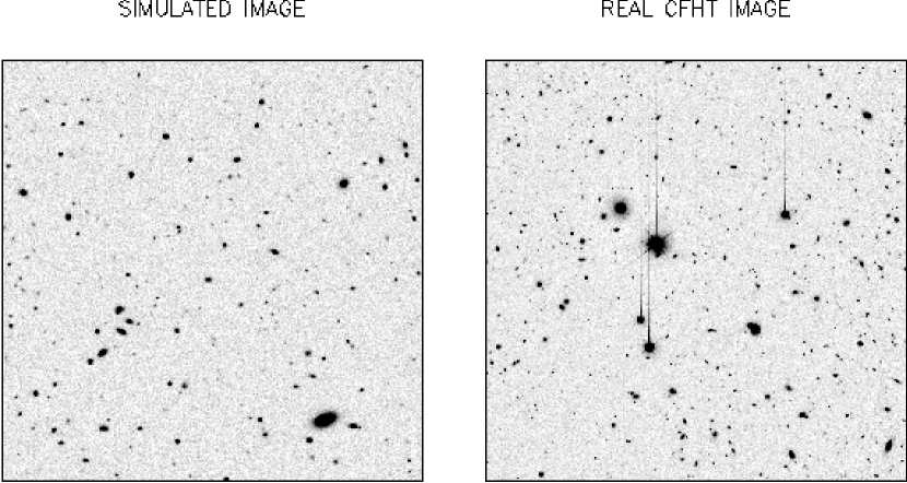
Figure 8: Simulated and real image sections $2^{\prime}.56$ on a side.

Figure 9: Catalogs from image sections shown in figure 8.

These data were analysed exactly like the real data. That is, the objects were detected as peaks of a smoothed image. The stars were extracted and their shapes fit in the manner described to obtain the PSF. A smoothed image $f_{s}=g\otimes f_{\rm o}$ was generated and from this the polarisation $q_{\alpha}$ was computed using (45), and the polarisability for each object was computed using (48).

References

- Allen (1973) Allen, C. 1973, Astrophysical Quantities (London: University of London, Athlone Press)
- Avila et al. (1997) Avila, R., Ziad, A., Borgnino, J., Martin, F., Agabi, A., & Tokovinin, A. 1997, Optical Society of America Journal, 14, 3070
- Bar-Kana (1996) Bar-Kana, R. 1996, ApJ, 468, 17
- Beckers (1993) Beckers, J. 1993, ARA&A, 31, 13
- Berry & Upstill (1980) Berry, M. V., & Upstill, C. 1980, Progress in Optics, 18, 257
- Bertin & Arnouts (1996) Bertin, E., & Arnouts, S. 1996, Astronomy and Astrophysics Supplement Series, 117, 393
- Bonnet & Mellier (1995) Bonnet, H., & Mellier, Y. 1995, A&A, 303, 331
- Born & Wolf (1964) Born, M., & Wolf, E. 1964, Principles of Optics (Oxford: Pergamon Press)
- Christian & Racine (1985) Christian, C., & Racine, R. 1985, PASP, 97, 1215
- Christou (1991) Christou, J. C. 1991, PASP, 103, 1040
- Coleman et al. (1980) Coleman, G. D., Wu, C.-C., & Weedman, D. W. 1980, ApJS, 43, 393
- Fischer & Tyson (1997) Fischer, P., & Tyson, J. A. 1997, AJ, 114, 14
- Fried (1966) Fried, D. L. 1966, J. Opt. Soc. Am., 56, 1372
- Gunn (1967) Gunn, J. 1967, ApJ, 147, 61
- Hoekstra et al. (1998) Hoekstra, H., Franx, M., Kuijken, K., & Squires, G. 1998, ApJ, 504, 636
- Jarvis & Tyson (1981) Jarvis, J. F., & Tyson, J. A. 1981, AJ, 86, 476
- Jenkins (1998) Jenkins, C. R. 1998, MNRAS, 294, 69
- Jorden et al. (1993) Jorden, P., Deltorn, J., & Oates, P. 1993, Gemini, 41, 1
- Jorden et al. (1994) Jorden, P., Deltorn, J.-M., & Oates, P. 1994, SPIE, 2198, 836
- Kaiser (1998) Kaiser, N. 1998, ApJ, 498, 26, http://xxx.lanl.gov/abs/astro-ph/9610120
- Kaiser et al. (1995) Kaiser, N., Squires, G., & Broadhurst, T. 1995, ApJ, 449, 460, http://xxx.lanl.gov/abs/astro-ph/9411005
- Kaiser et al. (1998) Kaiser, N., Wilson, G., Luppino, G., Kofman, L., Gioia, I., Metzger, M., & Dahle, H. 1998, ApJsubmitted, http://xxx.lanl.gov/abs/astro-ph/9809268
- Kochanek (1990) Kochanek, C. 1990, MNRAS, 247, 135
- Krist (1995) Krist, J. 1995, ASP Conf. Ser. 77: Astronomical Data Analysis Software and Systems IV, 4, 349
- Luppino & Kaiser (1997) Luppino, G., & Kaiser, N. 1997, ApJ, 475, 20, http://xxx.lanl.gov/abs/astro-ph/9601194
- Martin et al. (1998) Martin, F., Tokovinin, A., Ziad, A., Conan, R., Borgnino, J., Avila, R., Agabi, A., & Sarazin, M. 1998, A&A, 336, L49
- McClure et al. (1991) McClure, R. D., Fletcher, J. M., Arnaud, J., Nieto, J. L., & Racine, R. 1991, PASP, 103, 570
- McClure et al. (1989) McClure, R. D., et al. 1989, PASP, 101, 1156
- Mellier (1999) Mellier, Y. 1999, ARA&A, In press
- Roddier & Roddier (1993) Roddier, C., & Roddier, F. 1993, "J. Opt. Soc. Am. A", 10, 2277
- Roddier (1981) Roddier, F. 1981, Progress in Optics. Volume 19. Amsterdam, North-Holland Publishing Co., 19, 281
- Schneider et al. (1992) Schneider, P., Ehlers, J., & Falco, E. E. 1992, Gravitational lenses (New York: Springer-Verlag)
- Tatarski (1961) Tatarski, V. I. 1961, Wave propagation in a turbulent medium (New York: McGraw-Hill)
- Tonry et al. (1997) Tonry, J., Burke, B. E., & Schechter, P. L. 1997, PASP, 109, 1154
- Tyson et al. (1984) Tyson, J. A., Valdes, F., Jarvis, J. F., Mills, A. P., & , J. 1984, ApJ, 281, L59
- Valdes et al. (1983) Valdes, F., Jarvis, J. F., & Tyson, J. A. 1983, ApJ, 271, 431
- Wilson et al. (1996) Wilson, G., Cole, S., & Frenk, C. S. 1996, MNRAS, 280, 199
- Young (1974) Young, A. T. 1974, ApJ, 189, 587