Temperature and Emission-Measure Profiles Along Long-Lived Solar Coronal Loops Observed with TRACE

Abstract

We report an initial study of temperature and emission measure distributions along four steady loops observed with the Transition Region and Coronal Explorer (TRACE) at the limb of the Sun. The temperature diagnostic is the filter ratio of the extreme-ultraviolet 171 Å and 195 Å passbands. The emission measure diagnostic is the count rate in the 171 Å passband. We find essentially no temperature variation along the loops. We compare the observed loop structure with theoretical isothermal and nonisothermal static loop structure.

1 Introduction

The Transition Region and Coronal Explorer (TRACE) is producing a wealth of high-quality, high-cadence, high-resolution data for the solar corona in the extreme ultraviolet (Schrijver et al. (1996); Wolfson et al. (1997); Handy et al. (1999)) that allow us to probe the spatial and temporal structure of the corona in unprecedented detail.

The detailed properties of the corona are central to solving the coronal heating puzzle. Coronal loops are the most basic coronal structure, as evidenced by Yohkoh and most recently by TRACE. Theoretical studies of coronal structure and heating have thus focused on understanding loops (Landini & Monsignori Fossi (1975); Vaiana & Rosner (1978); Serio et al. (1981); Raymond & Foukal (1982); Jordan (1992); Ciaravella, Peres, & Serio (1993)). Previous and current EUV studies have found isothermal, hydrostatic loop structure (Gabriel & Jordan (1975); Aschwanden et al. 1999a, 1999b), while broadband X-ray analysis and theoretical calculations have suggested that coronal loops have temperature maxima at their tops (Rosner, Tucker, & Vaiana (1978); Serio et al. (1981); Kano & Tsuneta (1996)).

Here we report a first look at temperature and emission-measure structure along the axes of coronal loops observed with TRACE (Fig. 1). The temperature diagnostic we use is the 171 Å /195 Å filter ratio (Fig. 2a). The emission measure (EM) diagnostic is the 171 Å passband count rate (DN/s/pixel, DN$=$data number) (Fig. 2b), as calculated using the CHIANTI atomic database (Dere et al. (1997)).

2 Loop Observations

The data consist of observations in the 171 Å (Fe IX) and 195 Å (Fe XII) TRACE filters of four loop systems observed at the limb of the Sun (Fig. 1). The instrument resolution is 1$\farcs$0. We attempted to choose relatively isolated loops that extend above the limb of the Sun in order to minimize non-loop background flux and projection effects. Since we focus here on steady loop structures, the loops selected for measurement showed little morphological variation during the selected $1-2$ hour intervals (the loops were usually observed at high cadence for considerably longer times, up to six hours, but we restrict the time interval in an attempt to minimize effects of morphological evolution and of rotation onto and off of the limb). The data set for each loop thus consists of approximately one hour of high-cadence observations, each $10-40$ seconds long.

To investigate the variation of temperature along the loop, we then selected four subimages of each loop representing (1) an area near the base of the loop (roughly 1/5 of the distance to the loop top), (2) an area approximately 1/3 of the distance to the loop top, (3) an area approximately 2/3 of the distance to the loop top, and (4) an area roughly at the loop top. Rather than consider the entire loop length, we consider the half of each loop that shows the least overlap with adjacent structures. The subimage selection attempted to contain an adequate number of pixels from the loop of interest to spatially average, while excluding pixels from the background and/or adjacent coronal structure. Each subimage contains a few hundred to a few thousand pixels.

Precise loop length determinations would require analysis of possible projection effects; however, approximate loop lengths can be inferred from Figure 1. Rough estimates of the loop semilengths are $L=10^{10}$ cm for loops (a), (b), and (d) and $L=5\times 10^{9}$ cm for loop (c).

2.1 Data Reduction

The data were first inspected to remove rejection-quality images. The temperature determination uses the 171/195 filter ratio (Fig. 2a), so a sequence of 171-195 image pairs was extracted from each data set under the somewhat arbitrary constraint that each pair of images was obtained no more than two minutes apart. The resulting data set for each loop typically contains about 50 image pairs. The resulting intensity ratios were then coadded over the subimage and over the time sequence to produce a single intensity ratio, with associated error, for each data set. The 171-Å passband counts were similarly coadded to produce a single count rate per pixel, with associated error, for each data set.

Two types of errors result from this analysis. First, there are errors due to noise in the data, which we consider to be based on Poisson statistics of data with approximately 100 photons per data number. Second, there is an error associated with the width of the data distribution for each subimage; the distributions are approximately gaussian, and we take the corresponding error for each subimage to be one standard deviation of the data distribution for that subimage. For both the filter ratio and passband count diagnostics, the noise error and distribution error for each data set are on the order of fractions of a percent; we thus consider the errors to be negligible for the purposes of this study.

3 Results and Discussion

We first note some cautions/limitations regarding this analysis. First, in using the filter ratios to determine temperatures, we implicitly assume that all the material through which we look (i.e., integrated along the line of sight) at each position along the loop is at the same density and temperature. For this reason, we restrict ourselves to loop systems on the limb and measure relatively isolated loops. Second, analysis of the density structure along loops is conceptually difficult because of the intricate loop substructure evident in the images (Fig. 1).

The 171/195 filter ratios and 171-Å count rates for each loop as a function of fractional distance along the loop are given in Table 1. As inspection of Figure 2a indicates, the temperature as a function of the 171/195 filter ratio is multivalued in the coronal temperature range $\log(T)$ = $5-7$, so a definitive determination of the loop temperature is not possible based on these data alone (however, we note that the temperatures of maximum formation of the 171 and 195 lines are $\log(T)$ = 6.0 and 6.2, respectively, so it is tempting to conclude that the loop temperatures are around $\log(T)=6.1$). We note, however, that it is unlikely that the temperature profiles change along the loops, since transition from, e.g., $\log(T)=6.1$ to $\log(T)=6.4$ would result in observation of considerably lower intensity ratios at intermediate points along the loop than are observed. We thus conclude that there is no significant temperature variation along the loops we consider. Furthermore, Occam’s razor suggests that all the loops share the same temperature.

Theoretical loop models that include energy considerations predict a steep temperature rise in the transition region and a small, but measurable, temperature rise to a maximum at the loop top in the coronal part of the loop (see, e.g., Rosner et al. 1978; Serio et al. (1981)). In contrast, our observations show no significant temperature variation. Figure 3 shows the temperatures and emission measures for the observed loops and for three model loops: (1) an isothermal, hydrostatic loop with $T=1.34\times 10^{6}$ K, $L=10^{10}$ cm, a base emission measure of $6.25\times 10^{27}$ cm^-5, and uniform line-of-sight depth along the loop; (2) loop (1), but with a line-of-sight depth that increases gradually along the loop by a factor of 4; and (3) a static, steady-state, nonisothermal loop (cf. Serio et al. (1981)) that has $L=10^{10}$ cm, base pressure chosen such that the loop-top temperature agrees with that of the observed loops, and uniform line-of-sight depth of $10^{10}$ cm; for model loop (3), the base proton number density is $2.4\times 10^{10}$ cm^-3 and the base temperature is $2\times 10^{4}$ K.

Figure 3a shows the near-constant observed loop temperatures and the slight rise in the temperature structure of model loop (3). Figure 3b indicates that the observed emission-measure structure agrees better in its shape with the nonisothermal model (3) and in its magnitude with the isothermal models (1) and (2). If the observations accurately reflect the temperature and emission-measure structure in the loop, it may be that physical process(es) not included in our assumptions and model calculations exist in the observed loops. For example, the calculation for model loop (3) assumes a uniform volumetric heating rate, which may not describe actual loop heating. Furthermore, flows may introduce denser material into the loops, and mixing may homogenize the overall structure; alternatively, the hydrostatic pressure balance may be strongly affected by wave interactions with the background fluid (Litwin & Rosner (1998)).

The energetic requirements of the loops we have examined may range from $\sim 10^{5}-5\times 10^{6}$ erg s^-1 cm^-2, corresponding to line-of-sight depths of $10^{10}-10^{9}$ cm; “standard” values quoted in the literature are typically $\lesssim 10^{7}$ erg s^-1 cm^-2 (cf. Withbroe & Noyes (1977); Vaiana & Rosner (1978)). Smaller line-of-sight depths may be possible if the filling factor is small, as in the case of filamentary emission; such a configuration would correspond to a higher, localized (filamentary) energy input at the base, consistent with localized heating events such as microflares.

We do not measure any filter ratios consistent with transition-region temperatures of $\sim 10^{4}-10^{5}$ K; hence we conclude that the “footpoint” regions we choose lie above the transition region, a reasonable conclusion given that the transition region occupies roughly 3 pixels per image, and is likely to be obscured by absorbing material along the line of sight (Daw, DeLuca, & Golub 1995).

An earlier study of loop temperature distributions using Yohkoh X-ray data (Kano & Tsuneta (1996)) reports loop temperatures that increase from the footpoints to maxima at the loop tops by factors of $\gtrsim 1.2$. The loop temperature profiles we find vary by factors of at most 1.05. The temperatures they measured are higher by a factor of $3-5$ than the temperatures we report here. The lack of temperature variation in the EUV loops considered here (see also Gabriel & Jordan (1975); Aschwanden et al. 1999a, 1999b) invites speculation that there is a class of such isothermal loops distinct from loops with a temperature maximum at the apex. Whether the difference is due to some fundamental physical difference among loops, to a difference in the X-ray and EUV properties of loops, or to some other effect warrants further investigation.

Table 1: Loops Selected for Study

Loop Letter	Date/Time	171/195 filter ratio
(cf. Fig. 1)		and 171-Å count rate (DN/s/pixel)
		at fractional distance along loop
		0.2 ( $\sim$ base)	0.3	0.7	1.0 (apex)
a	04 Jul 98 1800-2000h	1.03	0.88	0.75	0.81
		10.01	6.22	3.92	3.12
b	26 Jul 98 2200-2300h	0.85	0.70	0.85	0.78
		4.68	2.87	2.51	1.93
c	18 Aug 98 1000-1100h	0.83	0.90	0.96	1.09
		11.39	9.74	9.32	9.18
d	20 Aug 98 0800-0900h	0.90	0.89	0.84	0.86
		10.20	7.50	5.84	6.35

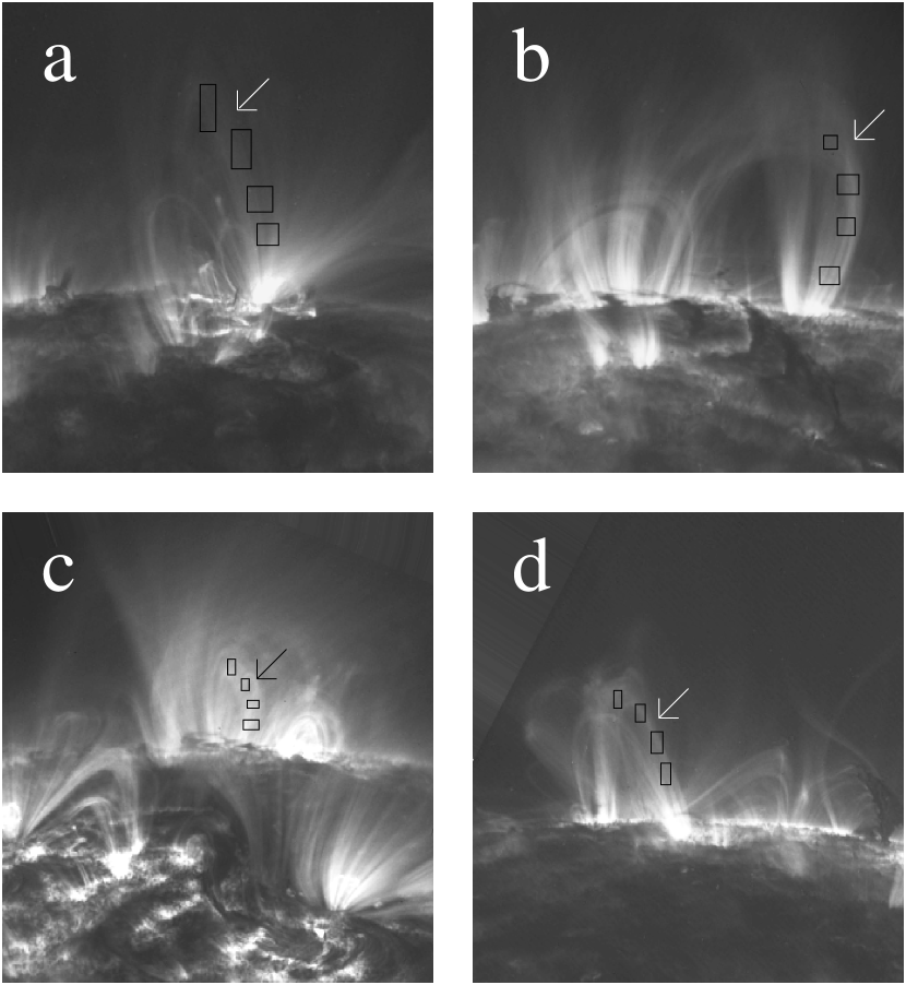
Figure 1: Images in the 171 Å filter of the loops selected for this study (indicated by arrows): (a) 04 Jul 1998, (b) 26 Jul 1998, (c) 18 Aug 1998, (d) 20 Aug 1998. Images have been rotated so that the limb is roughly horizontal. The field-of-view of each image is 5$\farcm$6 $\times$ 5$\farcm$4 (roughly 680 $\times$ 650 pixels). The rectangles represent the subimages used in this study.

Figure 2: (a) Filter ratio of TRACE 171 Å and 195 Å passbands; (b) Response of 171 Å passband in units of data number (DN) per second per pixel per emission measure (EM), where 1 DN $\approx 100$ photons and EM is in units of cm^-5.

Figure 3: Temperature (a) and emission measure (b) as functions of fractional distance along the loop for loop (a) (plus signs), loop (b) (diamonds), loop (c) (triangles), loop (d) (boxes), and model loop (3) with $T$(apex) = $1.34\times 10^{6}$ K and uniform line-of-sight depth $D=10^{10}$ cm (connected asterisks). Also shown in (b) are model loop (1): an isothermal ($T=1.34\times 10^{6}$ K), hydrostatic loop with a uniform line-of-sight depth (dashed line); and model loop (2): the same as model loop (1), but with a line-of-sight depth that increases along the loop by a factor of 4 (dot-dashed line). See §3 for discussion. The errors on the observations are comparable to or less than the size of the plot symbols.

References

- (1) Aschwanden, M. J., Alexander, D., Hurlburt, N., Newmark, J. S., Neupert, W. M., Klimchuk, J. A., & Gary, G. A. 1999b, in preparation
- (2) Aschwanden, M. J., Newmark, J. S., Delaboudinière, J.-P., Neupert, W. M., Klimchuk, J. A., Gary, G. A., Portier-Fozzani, F., & Zucker, A. 1999a, ApJ, in press
- Ciaravella, Peres, & Serio (1993) Ciaravella, A. A., Peres, G., & Serio, S. 1993, Sol. Phys., 145, 45
- Daw et al. (1995) Daw, A., DeLuca, E. E., & Golub, L. 1995, ApJ, 453, 929
- Dere et al. (1997) Dere, K. P., Landi, E., Mason, H. E., Monsignori Fossi, B. C., & Young, P. R. 1997, A&A Suppl. Ser., 125, 149
- Gabriel & Jordan (1975) Gabriel, A. H., & Jordan, C. 1975, MNRAS, 173, 397
- Handy et al. (1999) Handy, B. N., et al. 1999, Sol. Phys., submitted
- Jordan (1992) Jordan, C. 1992, Soc. Astron. Ital., 63, 605
- Kano & Tsuneta (1996) Kano, R., & Tsuneta, S. 1996, PASJ, 48, 535
- Landini & Monsignori Fossi (1975) Landini, M., & Monsignori Fossi, B. C. 1975, A&A, 42, 213
- Litwin & Rosner (1998) Litwin, C., & Rosner, R. 1998, ApJ, 506, L143
- Raymond & Foukal (1982) Raymond, J. C., & Foukal, P. 1982, ApJ, 253, 323
- Rosner, Tucker, & Vaiana (1978) Rosner, R., Tucker, W. H., & Vaiana, G. S. 1978, ApJ, 220, 643
- Schrijver et al. (1996) Schrijver, C., et al. 1996, BAAS, 28, 934
- Serio et al. (1981) Serio, S., Peres, G., Vaiana, G. S., Golub, L., & Rosner, R. 1981, ApJ, 243, 288
- Vaiana & Rosner (1978) Vaiana, G. S., & Rosner, R. 1978, ARA&A, 16, 393
- Withbroe & Noyes (1977) Withbroe, G. L., & Noyes, R. W. 1977, ARA&A, 15, 363
- Wolfson et al. (1997) Wolfson, J., et al. 1997, BAAS, 29, 887