CMB Anisotropy in
Compact Hyperbolic Universes

Abstract

Measurements of CMB anisotropy are ideal experiments for discovering the non-trivial global topology of the universe. To evaluate the CMB anisotropy in multiply-connected compact cosmological models, one needs to compute eigenmodes of the Laplace-Beltrami operator. We numerically obtain the eigenmodes on a compact 3-hyperbolic space cataloged as $m003(-2,3)$ in SnapPea using the direct boundary element method, which enables one to simulate the CMB in multiply-connected compact models with high precision. The angular power spectra $C_{l}$’s ($2\!\leq\!l\!\leq\!18$) are calculated using computed eigenmodes for $5.4\!\leq\!k<\!10$ and Gaussian random approximation for the expansion coefficients for $10\!\leq\!k\!<\!20$. Assuming that the initial power spectrum is the Harrison-Zeldovich spectrum, the computed $C_{l}$’s are consistent with the COBE data for $0.1\!\leq\!\Omega_{o}\!\leq\!0.6$. In low $\Omega_{o}$ models, the large-angular fluctuations can be produced at periods after the last scattering as the curvature perturbations decay in the curvature dominant era.

Introduction

The Einstein equation does not specify the global topology of the universe; therefore, there is no a priori reason to believe that the space-like hypersurface of the universe is simply-connected. If the space-like hypersurface is multiply-connected on the scale of the horizon or less, there is a possibility of discovering the multiply-connectedness by the future astronomical observations.
In recent years, there has been a great interest in properties of CMB anisotropy in multiply-connected cosmological models Ste ; deO2 ; Horn ; Flat ; Circles ; Circles2 ; Weeks . Precise measurements of the CMB anisotropy by the future satellite missions such as MAP and PLANCK may enable us to find the fingerprint of the multiply-connectedness in the CMB. Therefore, it is very important for us to simulate the CMB anisotropy in multiply-connected FRW models.
Constraints on the topological identification scales using the COBE data have been obtained for some flat models with no cosmological constant Ste ; Flat . The large-angular temperature fluctuations discovered by the COBE constrain the possible number of the copies of the fundamental domain inside the last scattering surface to less than $\!\sim$8 for these multiply-connected models.
The mode functions for flat models can be analytically obtained; therefore, the angular power spectra are obtained straightforwardly. On the other hand, no closed analytic expression of the eigenmodes is known for compact hyperbolic (CH) spaces. Therefore the analysis of the CMB anisotropy in CH models has been considered to be quite difficult. To overcome the difficulty, the author proposed a numerical approach called the direct boundary element method (DBEM) for computing eigenmodes of the Laplace-Beltrami operator Inoue . 14 eigenmodes have been computed for a ”small” CH space m003(-2,3) with volume $0.98139$ in the SnapPea catalog and it is numerically found that the expansion coefficients behave as if they are random Gaussian numbers.
We briefly describe the DBEM and the properties of the expansion coefficients which are used for computing the angular power spectra for low $\Omega_{o}$ CH cosmological models. We calculate the angular power spectra for m003(-2,3) using computed eigenmodes with small $k$, and an approximate method for eigenmodes with large $k$, which are compared with the COBE data.

Numerical Computation of Eigenmodes

The advantage of the DBEM is that it enables one to compute the eigenfunctions much precisely than other methods as it does not rely on the variational principle and it uses an analytical fundamental solution, namely the free Green’s function.
Let us first consider the Helmholtz equation on a compact connected and simply-connected M-dimensional domain $\Omega$ in a simply-connected M-dimensional Riemannian manifold $\cal{M}$ with appropriate periodic boundary conditions on the boundary $\partial\Omega$,

$$(\nabla^{2}+k^{2})u({\mathbf{x}})=0,$$ (1)

where $\nabla^{2}\equiv\nabla^{i}\nabla_{i},~{}(i=1,2,\cdot\cdot\cdot,M)$, and $\nabla_{i}$ is the covariant derivative operator defined on $\cal{M}$. A square-integrable function $u$ is the solution of the Helmholtz equation if and only if

$${\cal R}[u({\mathbf{x}}),v({\mathbf{x}})]\equiv\Bigl{\langle}(\nabla^{2}+k^{2})\ u({\mathbf{x}}),v({\mathbf{x}})\Bigr{\rangle}=0,$$ (2)

where $v$ is an arbitrary square-integrable function called weighted function and $\langle\,\rangle$ is defined as

$$\langle a,b\rangle\equiv\int_{\Omega}ab\,dV.$$ (3)

Then we put $u({\mathbf{x}})$ into the form

$$u=\sum_{j=1}^{M}u_{j}\phi_{j},$$ (4)

where $\phi_{j}$’s are linearly independent square-integrable functions. The best approximate solution can be obtained by minimizing the residue function $\cal R$ for a fixed weighted function $v({\mathbf{x}})$ by changing the coefficients $u_{j}$. Choosing the fundamental solution $G_{E}({\mathbf{x}},{\mathbf{y}})$ as the weighted function, Eq.(2) is transformed into a boundary integral equation,

$$c({\mathbf{y}})u({\mathbf{y}})+\int_{\partial\Omega}G_{E}({\mathbf{x}},{\mathbf{y}})\frac{\partial u}{\partial x^{i}}n^{i}\,\sqrt{g}\,dS-\int_{\partial\Omega}\frac{\partial G_{E}({\mathbf{x}},{\mathbf{y}})}{\partial x^{i}}n^{i}\,u\,\sqrt{g}\,dS=0,$$ (5)

where $c({\mathbf{y}})\!=\!1$ for ${\mathbf{y}}\!\in\!\Omega$ and $c({\mathbf{y}})\!=\!\frac{1}{2}$ for ${\mathbf{y}}\!\in\!\partial\Omega$. Since $\Omega$ is compact, the discrete eigenvalues are represented as $k_{0}\!=\!0<k_{1}<k_{2},\ldots$. The mode $k\!=\!k_{1}$ is the most important one that has the longest ”wavelength”defined as $2\pi/k$. The author succeeded in computing 14 eigenmodes for $k\!<\!10$ on m003(-2,3) Inoue . $k_{1}$ is numerically found to be 5.4.

From now on, we limit our consideration to CH spaces whose universal covering space is ${\cal{H}}^{3}$. We set the curvature radius of ${\cal{H}}^{3}$ to 1 without loss of generality. For convenience, we expand the eigenmodes $u_{\nu}$, ($\nu\!\equiv\!\sqrt{k^{2}-1}$) on the CH space in terms of eigenmodes $X_{\nu l}Y_{lm}$’s on ${\cal H}^{3}$,

$$u_{\nu}=\sum_{lm}\xi_{\nu lm}\,X_{\nu l}(\chi)Y_{lm}(\theta,\phi),$$ (6)

where $X_{\nu l}$ is a radial eigenfunction, $Y_{lm}$ is a spherical harmonic and $\xi_{\nu lm}$ is an expansion coefficient. It has been numerically found that $\xi_{\nu lm}$’s (for $l\!<\!19$ and $\nu\!<\!9.94$) behave as if they are random Gaussian numbers for m003(-2,3) , which is consistent with the prediction by random matrix theory. Random Gaussian behavior is also confirmed in a 2-dimensional CH space Aur1 . Note that some properties of a quantum system whose classical counterpart is a chaotic system can be explained by random matrix theory Bohigas . It has also been numerically found that the variance of $\xi_{\nu lm}$’s is proportional to $\nu^{-2}$. Using these properties, one can compute the approximate contribution from ”highly-excited” modes ($k\!>\!>\!1$) to the angular power spectrum.

Temperature Correlation

Temperature fluctuations in the multiply-connected FRW cosmological models can be written as linear combinations (using $\xi_{\nu lm}$ in the last section) of independent components of temperature correlations in the simply-connected FRW cosmological models. Assuming that the perturbations are adiabatic and super-horizon scalar type and the initial fluctuations are random Gaussian, the two-point temperature correlation in a CH cosmological model is written as

$$\Biggl{\langle}\frac{\delta T}{T}({\mathbf{n}})\frac{\delta T}{T}({\mathbf{n}}^{\prime})\Biggr{\rangle}\! = \!\!\sum_{l,m,\,l^{\prime},m^{\prime}}\bigl{\langle}a_{lm}a^{*}_{l^{\prime}m^{\prime}}\bigr{\rangle}Y_{lm}({\mathbf{n}})Y^{*}_{l^{\prime}m^{\prime}}({\mathbf{n}}^{\prime})$$ (7)

$$= \!\!\sum_{\nu,\nu^{\prime}\!,l,m,l^{\prime},m^{\prime}}\!\!\!\!\bigl{\langle}\Phi_{\nu}\Phi_{\nu^{\prime}}\bigl{\rangle}~{}\xi_{\nu lm}\xi^{\ast}_{\nu^{\prime}l^{\prime}m^{\prime}}L_{\nu lm}L^{\ast}_{\nu^{\prime}l^{\prime}m^{\prime}}\,,$$

where

$$\bigl{\langle}\Phi_{\nu}\Phi_{\nu^{\prime}}\bigl{\rangle}\!\! = \!\!\frac{4\pi^{4}~{}{\cal P}_{\Phi}(\nu)}{\nu(\nu^{2}\!+\!1)\textrm{Vol}(\Omega)}\delta_{\nu\nu^{\prime}},$$

$$L_{\nu lm}(\eta_{o},{\mathbf{n}})\! \equiv \!-Y_{lm}({\mathbf{n}})F_{\nu l}(\eta_{o}),$$

$$F_{\nu l}(\eta_{o})\!\! \equiv \!\!\frac{1}{3}\Phi_{t}(\eta_{\ast})X_{\nu l}(\eta_{o}\!-\!\eta_{\ast})\!+\!\!2\!\!\int_{\eta_{\ast}}^{\eta_{o}}\!\!\!\!\!\!d\eta\,\frac{d\Phi_{t}}{d\eta}X_{\nu l}(\eta_{o}\!-\!\eta),$$

$$\Phi_{t}(\eta)\!\! = \!\!\frac{5(\sinh^{2}\eta-3\eta\sinh\eta+4\cosh\eta-4)}{(\cosh\eta-1)^{3}}.$$

Here, ${\cal P}_{\Phi}(\nu)$ is the initial power spectrum, $\textrm{Vol}(\Omega)$ denotes the volume of the CH space and $\Phi_{\nu}$ and $\Phi_{t}(\eta)$ are the $\nu$-component and the time evolution of the Newtonian curvature perturbation, respectively. $\eta_{\ast}$ is the conformal time of the last scattering and $\eta_{o}$ is the present conformal time. The diagonal elements ($l\!=\!l^{\prime}$ and $m\!=\!m^{\prime}$) give the approximate angular power spectrum $\tilde{C}_{l}$ as

$$(2\,l+1)\,\tilde{C}_{l} = \sum_{m=-l}^{l}\langle~{}|a_{lm}|^{2}\rangle$$ (8)

$$= \sum_{\nu,m}\frac{4\pi^{4}~{}{\cal P}_{\Phi}(\nu)}{\nu(\nu^{2}+1)\textrm{Vol}(\Omega)}~{}|\xi_{\nu lm}|^{2}|F_{\nu l}|^{2}.$$

It should be noted that the non-diagonal terms (either $l\!\neq\!l^{\prime}$ or $m\!\neq\!m^{\prime}$) are not negligible for large angular (small l) fluctuations in anisotropic models such as CH models. Therefore, constrains on the models by using only the angular power spectra $C_{l}$ are not sufficient. On the other hand, this property can be considered as the ”fingerprint” of the multiply-connectedness of the spatial geometry of the universe.
Computation of highly-excited eigenmodes is still a difficult task since the number of the eigenmodes increases as $k^{3}$ and the number of the boundary elements increases as $k^{2}$. In order to avoid these difficulties, we assume that $\xi_{\nu lm}$ ’s are random Gaussian numbers and the variance is proportional to $\nu^{-2}$. Weyl’s asymptotic formula gives the approximate values of highly-excited eigenmodes

$$\tilde{\nu}(N)=\Biggl{(}\frac{6\pi^{2}N}{\textrm{Vol}(\Omega)}\Biggr{)}^{1/3},$$ (9)

where $N$ is an integer. We use pseudo-Gaussian random numbers $\xi_{\nu lm}$ that are derived from 14 eigenmodes on m003(-2,3) using the DBEM for $k\!<\!10$, and random Gaussian numbers $\xi_{\tilde{\nu}(N)lm}$ whose variance is proportional to $\nu^{-2}$ for $10\!\leq\!k\!<\!20$.
In FIGURE 1, $\delta T/T_{l}\!\equiv\![l(l+1)\tilde{C}_{l}/2\pi]^{1/2}$ is (diamonds) plotted with the COBE data analyzed by Gorski (stars) Gorski assuming that the initial power spectrum is the (extended) Harrison-Zeldovich spectrum ${\cal{P}}_{\Phi}(\nu)\!=\!Const$. The 1-$\sigma$ error bars are obtained by Monte-Carlo simulation with 10000 realizations. $\delta T/T_{l}$ is almost constant in the limit $\Omega_{o}$ to $1$ for the Harrison-Zeldovich spectrum. We see from these figures that $\delta T/T_{l}$ is almost flat for $0.2\!\leq\!\Omega_{o}\!\leq\!0.6$. Suppression of the large angular power due to the long ”wavelength” cutoff is quite mild compared with some flat multiply-connected models since the bulk of the large angular power comes from the decay of curvature perturbations well after the last scattering time, which is known as the integral Sachs-Wolfe effect. Considering the cosmic variance, the suppression of the large angular power for the $\Omega\!=\!0.1$ model is still within the acceptable range.

Summary

We numerically obtain 14 eigenmodes on a compact hyperbolic (CH) space m003(-2,3) with volume $0.98139$ using the direct boundary element method (DBEM). The temperature fluctuations are written in terms of the expansion coefficients $\xi_{\nu lm}$ and eigenmodes on the universal covering space. For the 14 eigenmodes, $\xi_{\nu lm}$’s are numerically found to be pseudo-random Gaussian numbers with variance proportional to $\nu^{-2}$.
The angular power spectra are computed using the 14 eigenmodes and an approximate method for eigenmodes with large k which is based on the assumption that the expansion coefficients are Gaussian random numbers. In contrast to multiply-connected flat models, the suppression of the large angular power is found to be so weak that the obtained powers are consistent with the COBE data for $0.1\!\leq\!\Omega_{o}\!\leq\!0.6$. Assuming that the initial perturbations are adiabatic, constraints on CH models are not so severe as long as one uses only the angular power spectra which contain only isotropic information.
However, one must also consider the anisotropic information of the temperature fluctuations. Contribution of the non-diagonal elements to the two-point temperature fluctuations is one of the key issues. Recently, Bond et al have obtained much severe constraints on the size of the topological identification scale for CH models using a method of imagesPogosyan . At the moment, the relation between their result and the author’s result is not clear. Various methods for extracting the anisotropic information have been suggested such as a search for circles in the sky Circles , or pattern formation Spots . The searches for the multiply-connectedness in the universe have just begun.

Acknowledgments

I would like to thank Kenji Tomita and Naoshi Sugiyama for their helpful discussions and continuous encouragements. I am supported by JSPS Research Fellowships for Young Scientists, and this work is supported partially by Grant-in-Aid for Scientific Research Fund (No.9809834).

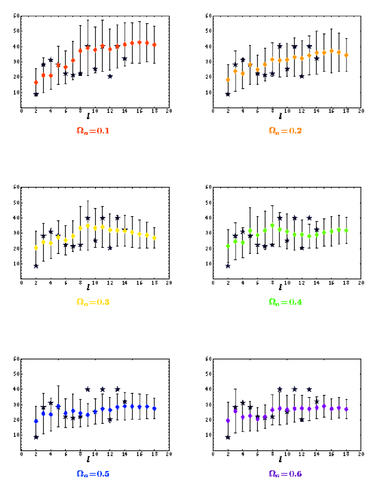
Figure 1: The diamonds show $\delta T/T_{l}$ in $\mu K$ for m003(-2,3) models with $0.1\!\leq\!\Omega_{o}\!\leq\!0.6$. The stars show the COBE data analyzed by Gorski(1996). The 1-$\sigma$ error bars are obtained from Monte-Carlo simulation with $N\!=\!10000$ realizations.

References

- (1)
- (2) Weeks, J.R., SnapPea:A computer program for creating and studying hyperbolic 3-manifolds, available at http://www.geom.umn.edu/software/download/snappea.html
- (3) Stevens, D., Scott, D. and Silk, J., Phys. Rev. Lett. 71, 20 (1993)
- (4) de Oliveira-Costa, A. and Smoot, G.F. and Starobinsky, A.A. ApJ 468, 457 (1996)
- (5) Levin, J.L., Barrow., J.D., Bunn, E.F. and Silk, J., Phys. Rev. Lett. 79, 974 (1997)
- (6) Scannapieco, E., Levin, J.L., and Silk, J., astro-ph/9811226
- (7) Cornish, N.J., Spergel D., and Starkman G., Phys. Rev. Lett. 77, ,215 (1996)
- (8) Cornish, N.J., Spergel D., and Starkman G. astro-ph/9708255
- (9) Weeks J.R., astro-ph/9802012
- (10) Inoue, K.T., astro-ph/9810034
- (11) Aurich, R. and Steiner, F., Physica D 64, 185 (1993)
- (12) Bohigas, O., ”Random Matrix Theories and Chaotic Dynamics” in Proceedings of the 1989 Les Houches School on Chaos and Quantum Physics, Giannoni, A.,et al eds., Elsevier, Amsterdam (1991)
- (13) Grski, K. M. et al, Astrophys. J. 464, L11 (1996)
- (14) Bond, J.R., Pogosyan, D., and Souradeep, T., astro-ph/9804041
- (15) Levin, J, et al, astro-ph/9807206