Inverse Compton Scattering in Mildly Relativistic Plasma

Abstract

We investigated the effect of inverse Compton scattering in mildly relativistic static and moving plasmas with low optical depth using Monte Carlo simulations, and calculated the Sunyaev-Zel’dovich effect in the cosmic background radiation. Our semi-analytic method is based on a separation of photon diffusion in frequency and real space. We use Monte Carlo simulation to derive the intensity and frequency of the scattered photons for a monochromatic incoming radiation. The outgoing spectrum is determined by integrating over the spectrum of the incoming radiation using the intensity to determine the correct weight. This method makes it possible to study the emerging radiation as a function of frequency and direction. As a first application we have studied the effects of finite optical depth and gas infall on the Sunyaev-Zel’dovich effect (not possible with the extended Kompaneets equation) and discuss the parameter range in which the Boltzmann equation and its expansions can be used. For high temperature clusters ($k_{B}T_{e}\gtrsim 15$ keV) relativistic corrections based on a fifth order expansion of the extended Kompaneets equation seriously underestimate the Sunyaev-Zel’dovich effect at high frequencies. The contribution from plasma infall is less important for reasonable velocities. We give a convenient analytical expression for the dependence of the cross-over frequency on temperature, optical depth, and gas infall speed. Optical depth effects are often more important than relativistic corrections, and should be taken into account for high-precision work, but are smaller than the typical kinematic effect from cluster radial velocities.

Subject headings: (cosmology:) cosmic microwave background — galaxies: clusters: general — methods: numerical — plasmas — scattering

1 Introduction

Inverse Compton scattering of the cosmic microwave background radiation (CMBR) by hot electrons in the atmospheres of clusters of galaxies, the Sunyaev-Zel’dovich (SZ) effect (Sunyaev and Zel’dovich 1980), has become a powerful tool in astrophysics. It is one of the most important secondary effects which cause fluctuations in the CMBR. We will refer to the effect arising from static gas as the static SZ (SSZ) effect, and that arising from gas with bulk motion as the kinematic SZ (KSZ) effect. Fluctuations in the CMBR caused by the SZ effects in an ensemble of clusters of galaxies should dominate on angular scales less than few arc minutes. The nature of these fluctuations depends on the evolution of clusters, and so it is a test of structure formation theories (eg. Aghanim et al. (1998); Molnar and Birkinshaw (1998)).

Observations of the SSZ effect, begun in the 1970s, have now become routine in the 90s with dedicated instruments using the latest receiver technology (for reviews see Rephaeli 1995b ; Birkinshaw (1999)). SZ effect and x-ray measurements probe the physical conditions in the intracluster gas in clusters of galaxies, and allow us to deduce the distance to the cluster without additional assumptions. This provides a useful independent method for determining the Hubble constant.

Observations of the KSZ effect are much more difficult since it is typically an order of magnitude smaller than the SSZ effect and has the same spectrum as the primordial fluctuations in the CMBR. The KSZ effect provides a method of measuring radial peculiar velocities of clusters, and even without the tangential velocity component, which might be determined using the Rees-Sciama (RS) effect (Rees and Sciama (1968); Birkinshaw and Gull (1983); Gurvits and Mitrofanov (1986); Aghanim et al. (1998); Molnar and Birkinshaw (1998)) it should provide important information on large scale velocity fields, which are closely related to the large scale density distributions and thus to the average total mass density in the Universe. Useful limits on the size of the KSZ effect for two clusters have recently been reported by Holzapfel et al. (1997a).

Most discussions of the SSZ effect have been based on non-relativistic calculations of its amplitude, made via a Fokker-Planck type expansion of the Boltzmann equation (Kompaneets (1957)). The advantage of this approach is that in interesting cases (electron temperature, $T_{e}$, much greater than the temperature of the incoming radiation) it provides a convenient analytical solution for the spectrum of the emerging radiation. However, it has been recognized recently that relativistic effects become important for clusters with $kT_{e}\gtrsim 10$ keV. Rephaeli (1995a) provided a relativistic solution for the SSZ effect as a series expansion in the optical depth ($\ll 1$ for clusters). There is no exact analytical solution. The numerical integrals involved are tractable in the single-scattering approximation, which is usually adequate in clusters. Fargion, Konoplich and Salis (1996) developed exact expressions for relativistic inverse Compton scattering of a laser beam with monochromatic isotropic radiation, finding good agreement with the approximations of Jones (1968). Their expression for the frequency redistribution function (FRDF) for scattering of mono-energetic electrons with monochromatic photons agrees with Rephaeli’s result. Rephaeli’s method has been used in a series of papers to evaluate the SSZ effect for hot clusters. Relativistic corrections to the SSZ effect, and to the standard thermal bremsstrahlung formulae, were applied to determine the Hubble constant in hot clusters by Rephaeli and Yankovich (1997), however, their corrections of the thermal bremsstrahlung equation were further corrected by Hughes and Birkinshaw (1998). Holzapfel et al. (1997b) used the relativistic results in their determination of the Hubble constant from observations of cluster Abell 2163.

The most general treatment of Compton scattering in static and moving media has been derived by Psaltis and Lamb (1997) as a series expansion. As Challinor and Lasenby (1998b) noted, however, more terms in the expansion should be taken into account for accurate treatment of clusters of galaxies. Recently the Kompaneets equation has been extended to contain relativistic corrections to the SSZ and KSZ effects (Stebbins (1997); Challinor and Lasenby 1998a , b; Itoh, Kohyama and Nozawa 1998; Nozawa, Itoh and Kohyama 1998; Sazonov and Sunyaev 1998b ). Starting from the Boltzmann equation, an expansion in the small parameters of the dimensionless temperature, $\Theta=kT_{e}/(m_{e}c^{2})$, fractional energy change in a scattering, $(h\nu^{\prime}-h\nu)/k_{B}T_{e}$, and dimensionless radial velocity for the KSZ effect, $v_{rad}/c$, leads to a Fokker-Planck type equation (the extended Kompaneets equation). Corrections up to the fifth order in $\Theta$ have been derived (Itoh et al. (1998)). These calculations demonstrate the importance of the relativistic effects (in accordance with the results of Rephaeli 1995a). Note however, that, as Challinor and Lasenby (1998a) emphasized, the extended Kompaneets equation is a result of an asymptotic series expansion, therefore it is important to estimate the validity of the expansion using other methods. Nozawa et al. compared the convergence of their expansion to a direct numerical evaluation of the Boltzmann collision integral, and concluded that in the Rayleigh-Jeans region the relativistic corrections give accurate results in the entire range of cluster temperatures. Significant deviations are found at higher frequencies for high temperature clusters.

The SSZ and KSZ effects must be separated in order to extract information on peculiar velocities. Fortunately the two effects have different frequency dependence. The maximum of the KSZ effect (in thermodynamic temperature units) occurs at about the “cross-over” frequency where the SSZ effect changes sign from being a decrement to an increment. In a non-relativistic treatment the cross-over frequency is a constant, 218 GHz, independent of electron temperature, optical depth, and all other parameters. Rephaeli (1995a) showed that in the relativistic case the cross-over frequency depends on the temperature, and his results were used by Holzapfel et al. (1997a) in determining peculiar velocities of two clusters. Sazonov and Sunyaev (1998b) and Nozawa et al. (1998) give approximations for the cross-over frequency as a function of dimensionless temperature and radial peculiar velocity. They also conclude that relativistic corrections to the cross-over frequency are important, and should be taken into account in future experiments.

Other methods have been used to investigate inverse Compton scattering, such as numerical integration of the collision integral (Corman (1970)), multiple scattering methods (Wright (1979)), and Monte Carlo simulations. Simulations of inverse Compton scattering in relativistic and non-relativistic plasma have been carried out for embedded sources (Pozdnyakov, Sobol, and Sunyaev 1983; Haardt and Maraschi (1993); Hua and Titarchuk (1995)). Gull and Garret (1998) used Monte Carlo methods to evaluate the Boltzmann collisional integral. Sazonov and Sunyaev (1998a) used Monte Carlo simulations to derive the SZ thermal and kinematic effects.

In this paper we study the effect of optical depth and non-uniform bulk motion on the SZ effect using a Monte Carlo method to calculate the frequency redistribution function. The inverse Compton scattering of CMBR photons is treated in the Thomson limit for static and infalling plasmas (SSZ and KSZ effects) with spherical symmetry, uniform density distribution, and low optical depth over a wide range of gas temperatures and observed frequency. We apply our results to clusters of galaxies assuming a static and radially infalling (or collapsing) gas component.

2 The Method

2.1 Formalism

The emerging intensity of a beam of radiation in the line of sight after passage through a scattering atmosphere can be expressed as a convolution of the FRDF and the incoming intensity:

$$I(x)=\int F(s)\,B(\nu_{0})\,ds,$$ (1)

where $x=h\nu/k_{B}T_{CB}$ is the dimensionless frequency, $B(\nu_{0})$ is the incoming intensity (hereafter assumed to be Planckian), and $F(s)$ is the FRDF, which specifies the probability of scattering from $\nu_{0}$ to $\nu$ as a function of the logarithm of the dimensionless frequency, $\nu/\nu_{0}$, $s=\ln(\nu/\nu_{0})$, where $h$, $\nu$, $k_{B}$ and $T_{CB}$ are the Planck constant, the frequency, the Boltzmann constant, and the temperature of the CMBR, $T_{CB}=2.728\pm 0.002$ K (Fixsen et al. (1996)). The FRDF can be expressed as

$$F(s)=e^{-\tau}\delta(s)+w_{sc}\,P(s),$$ (2)

where the first term containing the Dirac delta function, $\delta(s)$, describes the attenuated incoming radiation by a factor depending on the line of sight optical depth, $\tau$, the “out-scattered” radiation, and the second term describes the contribution from scattering into the beam, which depends on the FRDF of the scattered radiation, $P(s)$, and a weight, $w_{sc}$, which determines what fraction of the radiation scatters into the beam. This decomposition is possible because in our approximation the fractional frequency change is independent of the frequency (see equation 16 later). The change of the intensity in the line of sight may be expressed as

$$\Delta I(x)=\bigl{(}e^{-\tau}-1\bigr{)}B(x)+\int w_{sc}\,P(s)\,B(\nu_{0})ds.$$ (3)

For isotropic and homogeneous scattering conditions, so that the scattering parameters do not depend on where the scattering happens, the weight

$$w_{sc}=\bigl{(}1-e^{-\tau}\bigr{)},$$ (4)

which means that the out-scattered radiation is balanced by the same amount of in-scattered radiation, and so there would be no net intensity change ($\Delta I(x)=0$) if there were no frequency change ($P(s)$ is the Dirac delta function). Our task is to calculate $P(s)$ and $w_{sc}$. However, the assumption in equation (4) breaks down where the radiation field is not isotropic within the cloud, as will be the case in our static and collapsing models, or where there is relativistic bulk motion, which introduces anisotropy in the scattering via the relativistic beaming effect. In the cases which we discuss in the present paper, equation (4) is an excellent approximation as we have been able to verify using the results of our Monte Carlo simulations (see section 2.2). Significant departures from equation (4) will occur where the scattering optical depth becomes large, or where the gas velocities approach the speed of light: the appropriate treatment in these cases is discussed in a forthcoming paper. Our approximations are adequate for clusters of galaxies, thus we are going to assume the validity of equation (4) in the rest of this paper.

We derive $P(s)$ using a Monte Carlo method. At low optical depth ($\tau\lesssim 1$), the problem is suitable for Monte Carlo simulation because we do not have to follow photons through many scatterings in the medium (the average number of scatterings being approximately $\tau$). Although in this limit most of the photons do not scatter, and hence provide no information on $P(s)$, this is not a problem since we can use the method of forced first scattering (see below).

2.2 Monte Carlo Method

We give a short description of the method here, for a more detailed description see Molnar (1998).

We assume an isotropic incoming low temperature radiation field (the CMBR). We use forced first scatterings to study the inverse Compton process. The photons Compton scatter from an electron population with a relativistic Maxwellian distribution of momenta in the rest frame of bulk motion. We compute scattering probabilities in the rest frame of the electron in the Thomson limit (Chandrasekhar (1950)). This involves coordinate transformations from the observer’s frame to the rest frame of the bulk motion and to the rest frame of the electron. We assume time translation invariance and spherical symmetry. Time translational invariance is not exact for our model with infall, so that we make a snap-shot approximation. The error arising from this approximation is less than the light crossing time over the infall time ($\approx v_{r}/c=\beta_{r}$), which is only a few per cent of the infall term for our models.

In most cases we use the inverse method to generate the desired probability distribution. We use a rejection method when the inverse method leads to non-invertible functions or is too slow: for a general description of generating probability distributions cf. Pozdnyakov et al. (1983); Press et al. (1992). The former reference describes an alternative Monte Carlo method to treat inverse Compton scattering.

In the description that follows we use the word “photon” in the singular to refer to one Monte Carlo “photon”, one experiment in our simulation. We use a weight, $w_{in}$, to express the number of photons this one experiment represents (the weight does not have to be an integer). We carried out the simulation in five steps.

Step 1. The position and direction of incoming photons:

We assume that the photons arrive uniformly on a unit sphere (the radius of the gas is scaled to unity). In a coordinate system which is placed at the point of impact, the direction cosine of the incoming photons from the normal, $\mu_{in}$, can be sampled as

$$\mu_{in}=\sqrt{[RN]},$$ (5)

where we use $[RN]$ to indicate a uniformly distributed random number drawn each time when it occurs. The azimuthal angle is assumed to be uniformly distributed between 0 and $2\pi$.

Step 2. distance to the forced first scattering:

We use forced first scattering, which means that we take the probability of scattering equal to one on the photons’ original line of flight through the gas. Using the inversion method, the optical depth at which the incoming photon scatters becomes

$$\tau_{1}=-\ln\bigl{(}1-[RN]\cdot(1-e^{-\tau^{0}_{max}})\bigr{)},$$ (6)

where $\tau^{0}_{max}$ is the maximum optical depth in the line of sight (the superscript refers to the number of times the photon has already scattered; zero in this case). Since we are using forced first collisions, we have to account for the fraction of photons which are unscattered on their path through the cloud. The scattered weight may be obtained from equation (4): $w_{sc}=\bigl{(}1-e^{-\tau^{0}_{max}}\bigr{)}w_{in}$, and stays the same during subsequent (unforced) scatterings. The weight of the photons passing through the cloud without scattering is $w_{out}=w_{in}e^{-\tau^{0}_{max}}$.

Step 3. scattering:

At the calculated position of the (forced first) scattering, we use the direction of the incoming photon and obtain the direction of propagation and frequency of the scattered photon. In the case that the gas is moving, we make a Lorentz transformation into the rest frame of the moving plasma. We sample the scattered electron’s dimensionless velocity, $\beta_{e}=v_{e}/c$, from a relativistic Maxwellian distribution

$$P(\beta_{e})\,d\beta_{e}=N_{rel}\,\beta_{e}^{2}\,\gamma^{5}\,e^{-\gamma/\Theta}\,d\beta_{e},$$ (7)

where the normalization is

$$N_{rel}=\Bigl{(}\Theta\,K_{2}(1/\Theta)\Bigr{)}^{-1},$$ (8)

$K_{2}$ is the second order modified Bessel function of the second kind, and the dimensionless electron temperature is

$$\Theta={k_{B}\,T_{e}\over m_{e}c^{2}}.$$ (9)

We used the rejection method to sample $\beta_{e}$.

The distribution of the direction of electron momenta is simplest in a frame in which the photon momentum unit vector points into one of the coordinate axes, z for example. In this coordinate system the probability distribution of $\mu_{e}$, the cosine of the angle between the unit vector of the direction of photon propagation (z axis) and electron velocity, is

$$P(\mu_{e},\beta_{e})=(1-\beta_{e}\mu_{e})/2.$$ (10)

The inversion method leads to sampling $\mu_{e}$ as

$$\mu_{e}={1\over\beta_{e}}\Biggl{(}1-\sqrt{1-2\beta_{e}\biggl{(}2[RN]-1-{\beta_{e}\over 2}\biggr{)}}\Biggr{)},$$ (11)

where the sign of the square root was determined so that in the limit of small electron velocities we recover the result for an isotropic distribution ($\mu_{e}=2[RN]-1$). The angular distribution of the scattered electrons in the plane perpendicular to the momentum vector of the photon is isotropic (at azimuthal angle uniformly distributed between 0 and $2\pi$). In the rest frame of the electron, the cosine of the polar angle of the incoming photon is derived from a Lorentz transformation as

$$\mu={-\mu_{e}+\beta_{e}\over 1-\beta_{e}\mu_{e}},$$ (12)

where the negative sign in front of $\mu_{e}$ is appropriate for an incoming photon. In the electron’s rest frame the scattering probability of a photon coming in with direction cosine $\mu$ and leaving with direction cosine $\mu^{\prime}$ is given by Chandrasekhar (1950)

$$f(\mu,\mu^{\prime})={3\over 8}\Bigl{(}1+\mu^{2}\,{\mu^{\prime}}^{2}+{1\over 2}\bigl{(}1-\mu^{2}\bigr{)}\bigl{(}1-{\mu^{\prime}}^{2}\bigr{)}\Bigr{)}.$$ (13)

$\mu^{\prime}$ can be sampled using a uniform probability distribution by inversion of

$$[RN]={\int_{-1}^{\mu^{\prime}}f(\mu,\mu^{\prime})d\mu}={3\over 16}\biggl{(}\bigl{(}\mu^{2}-{1\over 3}\bigr{)}{\mu^{\prime}}^{3}+\bigl{(}3-\mu^{2}\bigr{)}\mu^{\prime}-{8\over 9}\biggr{)},$$ (14)

which leads to a cubic equation for $\mu^{\prime}$,

$$\Bigl{(}\mu^{2}-{1\over 3}\Bigr{)}{\mu^{\prime}}^{3}+\Bigl{(}3-\mu^{2}\Bigr{)}\mu^{\prime}-{8\over 3}\Bigl{(}2\,[RN]+{1\over 3}\Bigr{)}=0.$$ (15)

This cubic equation has a single real solution with absolute value of $\mu^{\prime}$ less or equal to one. We now transfer the direction and frequency of the scattered radiation back to the observer’s frame. The dimensionless outgoing frequency of the photon normalized to the incoming frequency (expressed with the $s$ parameter) becomes

$$s=\ln{\nu^{\prime}\over\nu_{0}}=\ln\Biggl{(}\gamma_{e}^{2}\Bigl{(}1-\beta_{e}\mu_{e}\Bigr{)}\Bigl{(}1+\beta_{e}\mu^{\prime}\Bigr{)}\Biggr{)}.$$ (16)

Step 4. loop over scatterings:

Having the point of scattering, the scattered frequency, and the direction of the scattered photon, we now sample the optical depth to the next scattering. We do not use forced scattering, so the optical depth follows from the usual (inverse) method as

$$\tau_{n}=-\ln[RN],$$ (17)

where the lower index on $\tau$ refers to the $n$th scattering ($n>1$), and we used $[RN]=1-[RN]$, which is correct for uniform probability distributions. If $\tau$ is less than the maximum optical depth in the direction of the photon momentum after the previous scattering, $\tau^{n-1}_{max}$, the photon is taken to have scattered within the cloud, and we calculate the new scattering direction and frequency of the scattered photon as in step 3. If $\tau_{n}>\tau^{n-1}_{max}$, the photon escaped (scattered $n-1$ times), and we register the impact parameter (the distance between the line of sight and the center of the spherically symmetric scattering medium), the weight of the photon, the number of scatterings and $s$, the dimensionless frequency of the escaped photon.

Step 5. The frequency redistribution function:

At the end of the simulation we sum the weights in every impact parameter bin to check our assumption of homogeneous scattering (equation 4) and we determine how the average number of scatterings depend on the impact parameter. It turns out that, in our case of low optical depth and very mild infall velocities, the average number of scatterings has no noticeable dependence on the impact parameter, and that equation (4) is satisfied at each impact parameter within the accuracy of our Monte Carlo simulations, which is less than 0.1 %. The scattered FRDF depends only on the number of scatterings, thus we can sum all the photons to determine an average scattered FRDF, which can be used as an excellent approximation to the FRDF corresponding to an arbitrary line of sight.

Therefore the discrete probability distribution of the scattered FRDF can be derived by binning the frequencies of all the out-coming photons as

$$P(s_{k})=N_{s}\,{\cal N}_{k}.$$ (18)

${\cal N}_{k}$ is the number of photons in the k^th bin, for which ${s_{k}-\Delta s/2}\leq s<{s_{k}+\Delta s/2}$, where $s_{k}$ is the center of the k^th bin, $\Delta s$ is the width of the bin, and $N_{s}$ is the normalization, $N_{s}=1/(\Delta sN_{MC})$. $N_{MC}$ is the number of Monte Carlo photons. This $P(s_{k})$ is our sampled approximation to $P(s)$, and we then fit an exponential of polynomials to $P(s_{k})$ to get a convenient expression for the FRDF. Our fit gives an approximation accurate to better than half a percent, except in the (small) extended tails, where $P(s)$ is under-represented. However, these regions lie 3 orders of magnitude below the peak, and the error arising from the fit is negligible for our applications.

2.3 Testing the code

2.3.1 Single-scattering approximation

We tested our code by comparing our single scattering Monte Carlo results for the FRDF ($P_{1}^{MC}$) to those derived from Rephaeli (1995a). Rephaeli’s single-scattering approximation can be written as

$$P_{1}(s)={3\over 32\,N_{rel}}\,\int_{\beta_{0}}^{1}\gamma\,e^{-\gamma/\Theta}\beta_{e}^{-4}\bigl{(}f_{1}+f_{2}+f_{3}\bigr{)}\,d\beta_{e},$$ (19)

where the lower limit $\beta_{0}$ is the minimum $\beta_{e}$ needed to get the frequency shift $s$,

$$\beta_{0}={e^{|s|}-1\over e^{|s|}+1}.$$ (20)

The functions $f_{1}$, $f_{2}$ and $f_{3}$ are

$$f_{1} = e^{3s}\beta_{e}^{3}\bigl{(}\mu_{2}^{3}-\mu_{2}-\mu_{1}^{3}+\mu_{1}\bigr{)}$$ (21)

$$f_{2} = \biggl{(}\beta_{e}^{2}-3\bigl{(}4e^{s}+1\bigr{)}+3\,e^{s}(x_{2}+x_{1})+{2\beta_{e}^{2}-3(1+\beta_{e}^{4})\over x_{2}\,x_{1}}\biggr{)}e^{s}\,(x_{2}-x_{1})$$ (22)

$$f_{3} = 2e^{s}\,\bigl{(}e^{s}+1\bigr{)}\bigl{(}3-\beta_{e}^{2}\bigr{)}\ln{x_{2}\over x_{1}},$$ (23)

where $x_{1}=1-\beta_{e}\,\mu_{1}$, $x_{2}=1-\beta_{e}\,\mu_{2}$, $\mu_{1}$ and $\mu_{2}$ are defined by

$$\mu_{1} = \cases{-1&$s\leq 0$\cr{1-e^{-s}(1+\beta_{e})\over\beta_{e}}&$s\geq 0$\cr}$$ (24)

$$\mu_{2} = \cases{{1-e^{-s}(1-\beta_{e})\over\beta_{e}}&$s\leq 0$\cr 1&$s\geq 0$\cr},$$ (25)

and we used equation (16) to eliminate $\mu\prime$. This result (equation 19) agrees with Fargion et al. (1996). These expressions can be integrated numerically, except when $s=0$. In that case $\beta_{0}=0$, and direct numerical integration is not possible because of the diverging $\beta_{e}^{-4}$ term. For small $\beta_{e}$ ($\beta_{e}<b=0.1$ for example) we can expand the logarithm, and use this expansion as a good approximation. For $s=0$, equation (19) becomes

$$P_{1}(s=0)={3\over 8\,N_{rel}}\,\Biggl{(}\int_{0}^{b}f_{0}\,d\beta_{e}+\int_{b}^{1}f_{0}\,d\beta_{e}\Biggr{)},$$ (26)

where the integrand is

$$f_{0}=\gamma\,e^{-\gamma/\Theta}\beta_{e}^{-4}\Biggl{(}2\gamma^{2}\,\beta_{e}^{5}+6\beta_{e}+(3-\beta_{e}^{2})\ln\Bigl{(}{1-\beta_{e}\over 1+\beta_{e}}\Bigr{)}\Biggr{)}.$$ (27)

A Maclaurin expansion of the logarithm to order $\beta_{e}^{4}$ gives an adequate approximation

$$\int_{0}^{b}f_{0}\,d\beta_{e}\approx\int_{0}^{b}\gamma\,e^{-\gamma/\Theta}\beta_{e}\,\biggl{(}\gamma^{2}+{1\over 3}-{3\over 5}+\Bigl{(}{1\over 5}-{3\over 7}\Bigr{)}\beta_{e}^{2}+\Bigl{(}{1\over 7}-{1\over 3}\Bigr{)}\beta_{e}^{4}\biggr{)}\,d\beta_{e}$$ (28)

with no remaining divergent terms for the first integral in equation (26).

We derive $P_{1}^{MC}(s)$ from our Monte Carlo simulation by using the results of only the first (forced) scatterings. Figures 1a and 1b show our Monte Carlo results, $P_{1}^{MC}$, superimposed on $P_{1}$ from equations (19) and (21) for dimensionless temperatures $\Theta=0.03$ and 0.3. The agreement is excellent, confirming that our Monte Carlo code is successfully reproducing $P_{1}(s)$.

2.3.2 Testing the Numerical Integral for the Intensity Change

We derive the intensity change from the FRDF using a numerical integral (equation 3). The Kompaneets approximation leads to the following FRDF:

$$F_{K}={1\over\sqrt{4\pi y}}\exp\Bigl{(}-{(s-3y)^{2}\over 4y}\Bigr{)},$$ (29)

where the Compton $y$ parameter is

$$y=\int n_{e}\sigma_{T}\,\Theta d\ell,$$ (30)

where $n_{e}$ is the electron number density as a function of length in the line of sight measured by $\ell$ and $\Theta$ is the dimensionless temperature (for a discussion see for example Birkinshaw (1999); Molnar (1998)). In order to check our numerical method, we used the Kompaneets FRDF (equation 29) in the numerical integral in equation (3), and compared the resulting intensity change to that of obtained by the analytic solution for the Kompaneets approximation

$$\Delta I_{K}=y\,{\imath_{0}x^{4}e^{x}\over(e^{x}-1)^{2}}\biggl{(}x{e^{x}+1\over e^{x}-1}-4\biggr{)},$$ (31)

where $\imath_{0}=2(k_{B}T_{CB})^{3}/(hc)^{2}$. We concluded that our numerical method is accurate better than 0.1%.

2.3.3 Relativistic Corrections to Kompaneets equation

We also compare our results to those from the extended Kompaneets equation up to the 5th order in $\Theta$ (Itoh et al. (1998)). Itoh et al. expressed the intensity change as

$$\Delta I={\Delta n\over n}{\imath_{0}x^{3}\over e^{x}-1},$$ (32)

and provided expressions for ${\Delta n\over n}$ (note, that their $y$ parameter is actually $\tau$, the optical depth). On Figure 2 we plot $\Delta I/\tau$ from the Kompaneets approximation, from Itoh et al.’s expansion, and for our single scattering Monte Carlo results. From the figure we conclude that our single scattering Monte Carlo result agrees with that of Itoh et al. at low temperatures, $\Theta<0.03$ ($T_{e}<15$ keV). Deviations from the Itoh et al.’s result are already appearing at $\Theta=0.03$, and become more pronounced at higher temperatures and high frequencies, as we would expect.

We conclude that our simulation method passes these two tests, and can now be used to calculate the effects of multiple scattering and bulk velocity on the SZ effect.

3 Results

We performed a number of simulations for uniform density spherical models which are either static or have radial infalls with constant gas velocity at all radii. These models cover a range of $\tau_{0}$, the optical depth of zero impact parameter, electron temperature, $T_{e}$, and gas infall speed, $\beta_{r}$. Simulations with monochromatic incoming radiation were used to determine the scattered FRDF.

We verified via our simulations that for our low optical depth static models and for our models with low optical depth and very mild infall velocities, a parameter space adequate for clusters of galaxies, the dependence of the scattered FRDFs on the impact parameter is negligible, and that equation (4) provides a very good approximation to the weight of the scattered radiation. Although we determined an averaged scattered FRDF from all scattered photons regardless of their impact parameter, in our case, the determined scattered FRDF can be used at any impact parameter, since the dependence of the average number of scatterings on the impact parameter is negligible (see section 2.2, Step 5).

In Figure 3 we show the FRDFs of scattered photons emerging from our spherical static models with maximum optical depth $\tau_{0}=0.05$ and seven different temperatures. We used all photons to derive the scattered FRDFs. At higher temperatures more photons scatter into higher energies, thus the FRDFs are broader, and have lower peaks (since they are normalized to unity). We show the effect of finite optical depth in Figure 4: higher optical depth leads to more scatterings, and therefore more photons scattered to higher energies. Even for an optical depth as large as $\tau_{0}=0.1$ the change in the function is relatively small. In Figure 5 we show the effect on the FRDF of gas infall. Larger infall velocities cause more up-scattering of the photons, and hence more spreading of the FRDF, but the most obvious change is that the sharp peak at $s=0$ is smoothed out by the motion of the plasma. At lower temperatures bulk motion causes larger departures from the static FRDF since the infall speed is larger relative to the electron thermal velocity.

We used these results for the scattered FRDF to calculate intensity change using equations (3) and (4). We evaluated the emergent intensity change at zero impact parameter (i.e. through the center of the gas sphere), where $\tau=\tau_{0}$. In Figure 6 we show the intensity change $\Delta I$ for a static plasma for two optical depths and five temperatures. Non-zero optical depth causes only slight changes in the emerging radiation. Figure 7 shows the intensity change for a plasma with infall for two infall velocities and three plausible cluster temperatures. Only small changes in the spectrum are apparent, even with such large velocities.

One measure of the spectral deformation that has been used to quantify relative correction, and which is of use in determining the frequency at which to search for the KSZ effect, is the cross-over frequency. Challinor and Lasenby (1998a) and Birkinshaw (1998) suggested a linear expression for how the frequency changes with temperature, as

$$X^{lin}_{0}=3.830(1+1.13\,\Theta),$$ (33)

while Itoh et al. (1998) suggested a quadratic approximation

$$X^{q}_{0}=3.830(1+1.1674\,\Theta-0.8533\,\Theta^{2})$$ (34)

for most cluster temperatures. In Figure 8 we compare our Monte Carlo results with these and other expressions that include relativistic corrections. Our Monte Carlo results for single scattering are close to those obtained by numerical integration of the collision integral (Nozawa et al. (1998)). Relativistic corrections of third and fifth order (Challinor and Lasenby 1998a ; Nozawa et al. (1998)), or the linear approximation (Challinor and Lasenby 1998a ; Birkinshaw (1999)) are of varying accuracy in describing the curve: the linear and third order expressions give the best results, but extending the series to the fifth order is much poorer. This is a consequence of the asymptotic nature of the series, as emphasized by Challinor and Lasenby (1998a).

Figures 9 and 10 show the cross-over frequency as a function of dimensionless temperature $\Theta$ for finite optical depth and infall velocity. Including a finite optical depth causes only a small change in the $X_{0}(\Theta)$ curve, and this change does not depend much on temperature. Based on our Monte Carlo simulations, we suggest the following approximation for the cross-over frequency for single scatterings in static spherical plasma for dimensionless temperature $\Theta\lesssim 0.3$:

$$X_{0}^{s}(\Theta)=3.827\,(1+1.2038\,\Theta-1.2567\,\Theta^{2}+0.9098\,\Theta^{3}),$$ (35)

which fits better than 0.01 % in this range with a shift from the optical depth dependence

$$\Delta X_{0}^{\tau}(\tau_{0})=\tau_{0}\bigl{(}0.35-0.04416\,\Theta^{-0.5}\bigr{)},$$ (36)

which fits better than 0.005 % for $0.05\leq\Theta\leq 0.3$, and about 0.1 % for lower temperatures, and $\tau_{0}<0.5$.

Figure (10) shows results for our spherical models with gas infall. As for non-zero optical depth, additional energy transfers occur because of motion of the gas. As we would expect, at low temperatures the contribution to the electron velocity from bulk motion is comparable to that from thermal motion, and an enhanced frequency shift results, while at high temperatures this contribution becomes negligible. Based on our Monte Carlo simulations, we suggest the following approximation for the cross-over frequency shift in plasma with infall for $0.01\leq\Theta\leq 0.3$:

$$\Delta X_{0}^{\beta}(\Theta,\beta_{r})=0.224\,\beta_{r}^{2}\,\Theta^{-0.7}.$$ (37)

This formula fits the cross over frequency $\nu_{0}$ better than about half a percent.

At small optical depth and bulk velocity we can assume that the shifts simply add, so that the final expression for the cross-over frequency becomes

$$X_{0}(\Theta,\tau_{0},\beta_{r})=X_{0}^{s}(\Theta)+\Delta X_{0}^{\tau}(\tau_{0})+\Delta X_{0}^{\beta}(\Theta,\beta_{r}).$$ (38)

In Figure 11 we show the cross-over frequency as a function of temperature and optical depth in the parameter range ($\Theta\lesssim 0.04$, $\tau_{0}\lesssim 0.05$) important for clusters of galaxies. From this figure we may come to the conclusion that, for clusters of galaxies, the optical depth effect on the cross-over frequency is more important than non-linear terms in the expansion in $\Theta$. We provide more accurate fitting formulae for this range. From our models we find

$$X_{0}^{cl}(\Theta,\tau_{0},\beta_{r})=3.829\,(1+1.1624\,\Theta-0.68948\,\Theta^{2})+0.14\,\tau_{0}+\Delta X_{0}^{\beta}(\Theta,\beta_{r}),$$ (39)

which fits better than 0.03 % for static models in this range of parameters. The optical depth independent first term is similar to the approximation provided by Itoh et al. (1998), which was obtained by numerically integrating the collision integral.

The relativistic corrections to the kinematic SZ effect (cluster radial bulk velocity, $v_{rad}$) have also been found to be important (Nozawa et al. (1998), Sazonov and Sunyaev 1998b ) The shift was found to be

$$\Delta X_{0}^{kin}(\Theta,v_{rad})=300\,{v_{rad}\over c}\biggl{[}{a_{1}\over\Theta-\Theta_{min}}+{a_{2}\over(\Theta-\Theta_{min})^{2}}+a_{3}+a_{4}\,\Theta+a_{5}\,\Theta^{2}\biggr{]},$$ (40)

where $v_{rad}$ is the radial velocity, $\Theta_{min}=1.654\times 10^{-3}$, $a_{1}=3.857\times 10^{-3}$, $a_{2}=-4.631\times 10^{-6}$, $a_{3}=1.370\times 10^{-2}$, $a_{4}=1.014\times 10^{-2}$, and $a_{5}=0.01$ (Nozawa et al. (1998)), which agrees well with Sazonov and Sunyaev’s (1998b) result (expressed by a different fitting function). In Figure 11, long dashed lines represent the results of this kinematic effect of cluster radial velocity of $\pm$ 100 $\rm km\,s^{-1}$  ($X_{0}^{cl}(\Theta,0)+\Delta X_{0}^{kin}(\Theta,v_{rad})$) Comparing our results for the shift in the cross-over frequency to results from relativistic kinematic effect, we conclude that a shift caused by an optical depth of 0.01 is equivalent to a shift caused by a radial velocity of about $v_{rad}=-10$ $\rm km\,s^{-1}$.

We estimate the amplitudes of these effects on the hot cluster, Abell 2163, which was discussed by Holzapfel et al. (1997a). The maximum optical depth of the cluster is $\tau_{0}=0.01$, the temperature of the intracluster gas is close to $\Theta=0.03$. Using our results for the static effect with the given temperature and maximum optical depth we get about 100 MHz shift to higher frequencies relative to the linear expression of Challinor and Lasenby (1998a). An infall velocity of $\beta_{r}=0.01$ causes about an additional 15 MHz shift to higher frequencies relative to our result for the static model. These shifts are small relative to the 20 GHz band width of the instrument of Holzapfel et al. (1997a) and the error in $H_{0}$ and cluster radial peculiar velocity from ignoring their presence would be about 10 % (if the SZ effect is measured at $x\gtrsim 5$) and 15 $\rm km\,s^{-1}$. By comparison, the component of primordial anisotropy in this scale corresponds to adding a velocity noise about $\pm\,200$ $\rm km\,s^{-1}$.

4 Conclusions

We investigated the effect of finite optical depth and bulk motion on inverse Compton scatterings in spherically symmetric uniform density mildly relativistic plasma. We assumed isotropic incoming radiation (CMBR), a relativistic Maxwellian distribution for the electron momenta, and scatterings in the Thomson limit. We demonstrated the usefulness of our Monte Carlo method for solving the radiative transfer problem, and calculated the static and kinematic SZ effects with different optical depth and gas infall velocities.

The solution of the extended Kompaneets equation (with corrections up to the fifth order) is equivalent to a single-scattering approximation, and significant deviations from it occur for hot clusters and at high frequencies. These deviations may be as large as 5 % of the intensity change and neglecting them could cause about a 10 % error in the Hubble constant. A finite optical depth causes further small changes in the SZ effect: these changes may exceed the relativistic correction terms. For typical cluster temperatures, an accurate expression for the cross-over frequency as a function of temperature, optical depth, and bulk motion is (39).

As it can seen from Figure 11, the cross-over frequency is sensitive to the cluster radial velocity, and less sensitive to the finite optical depth. Measurements of the cross-over frequency can, in principle, be used to determine the radial velocity of the cluster (e.g., as in Holzapfel et al. 1997b ), with small extra corrections for optical depth and possible gas motion inside the cluster. However, the relatively strong variation of $X_{0}$ with $\Theta$, compared to $\tau$ or $\beta_{r}$, suggests that the largest uncertainty will arise from the assumption of cluster isothermality, even if effects of confusion from primordial (and secondary) CMBR fluctuations can be excluded.

Finally we note that our method can be extended to any geometry, density distribution and complicated bulk motion as desired, and may be used to study the SZ effect in high temperature plasmas with or without bulk motion.

Figure 1: The frequency redistribution function, $P(s)$, for a static, single scattering case at dimensionless temperatures $\Theta=0.03$ (a), or $\Theta=0.3$ (b). The solid line shows the result from Rephaeli 1995b)’s semi-analytic method, the boxes with vertical error bars (too small to be visible) show results from our Monte Carlo simulations.

Figure 2: The intensity change $\Delta I/\tau$ (in units of $\imath_{0}=2(k_{B}T_{CB})^{3}/(hc)^{2}$) as a function of dimensionless frequency $x=h\nu/(k_{B}T_{CB})$ for dimensionless temperatures $\Theta=0.01$, 0.02, and 0.03 in static spherically symmetric models. The solid, dashed and dotted lines are results from Monte Carlo method (single scattering), from relativistic corrections to the Kompaneets approximation (Itoh et al. 1997) and the Kompaneets approximation (Kompaneets 1957) respectively. Note that at low temperatures, $\Theta=0.01$ and 0.02, the single scattering Monte Carlo method and the Kompaneets approximation with relativistic corrections give very similar results (the solid and dashed lines overlap).

Figure 3: Scattered frequency redistribution functions, $P(s)$-s, of scattered photons emerging from our spherical static models with maximum optical depth $\tau_{0}=0.05$ and seven different temperatures. We used all emerging photons to determine $P(s)$ regardless of their impact parameter. (see text for details). The higher the temperature, the lower the peak and wider the function due to larger energy transfers from the hot electrons to the photons.

Figure 4: The inner part of the scattered frequency redistribution function, $P(s)$, for static clusters with dimensionless temperatures $\Theta=0.01$, 0.02, and 0.03. The solid and dashed lines show the extremes of single scattering and scattering with maximum optical depth $\tau_{0}=0.1$. More scatterings lead to more energetic photons, and hence more scattering from the line center to the high energy tail.

Figure 5: The single scattering frequency redistribution function, $P(s)$, for infalling plasma with dimensionless temperatures $\Theta=0.01$, 0.02 and 0.03. The solid, dashed and dashed dot lines show results for models with infall velocities $\beta_{r}=0$ (static), 0.03, and 0.05.

Figure 6: The intensity change $\Delta I/\tau$ (in units of $\imath_{0}=2(k_{B}T_{CB})^{3}/(hc)^{2})$) as a function of dimensionless frequency $x=h\nu/(k_{B}T_{CB})$ for five dimensionless temperatures in static spherically symmetric models, for single scattering (solid lines) and $\tau_{0}=0.1$ (dashed lines).

Figure 7: The intensity change $\Delta I/\tau$ (in units of $\imath_{0}=2(k_{B}T_{CB})^{3}/(hc)^{2})$) as a function of dimensionless frequency $x=h\nu/(k_{B}T_{CB})$ for three dimensionless temperatures in spherically symmetric models with infall. Monte Carlo results are plotted using single scattering approximation for static gas (solid line) and gas with bulk motion ($\beta_{r}=0.05$, dashed line).

Figure 8: The cross-over frequency as a function of dimensionless temperature, $\Theta$. The solid and long dashed lines show our Monte Carlo results for single scattering, and the results of a numerical evaluation of the collision integral (Nozawa et al 1998). The dashed dot line represents a linear approximation (Challinor and Lasenby 1998a; Birkinshaw 1998). The short dashed and dashed dot dot dot lines use relativistic corrections of third and fifth order in $\Theta$.

Figure 9: The cross-over frequency as a function of dimensionless temperature, $\Theta$ for static, spherically symmetric plasma. The solid and dashed lines are our results for single scattering and $\tau_{0}=0.1$, respectively. The dashed dot line shows a linear approximation (Challinor and Lasenby 1998a; Birkinshaw 1998). Finite optical depths cause a shift due to multiple scattering which is almost independent of the temperature.

Figure 10: The cross-over frequency as a function of dimensionless temperature, $\Theta$, for our spherically symmetric model with infall. The solid and dashed lines are for infall velocities $\beta_{r}=0$ (reference static model) and $\beta_{r}=0.05$. We used single scattering results to show only bulk motion effects. The dashed dot line shows a linear approximation (Challinor and Lasenby 1998a; Birkinshaw 1998). The effect of infall becomes inconsequential at high temperature since the infall speed becomes negligible relative to the thermal speed of the electron.

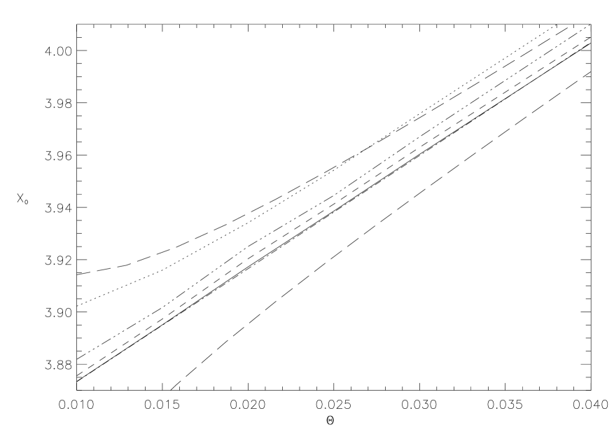
Figure 11: The cross-over frequency as a function of dimensionless temperature, $\Theta$, for several optical depths in a static spherical plasma. Our Monte Carlo results are from single scattering (solid line), $\tau_{0}=0.02$ (short dashed line), 0.05 (dash, dot, dot, dot line), and 0.1 (dotted line). The dash-dot line, which is hardly distinguishable from the solid line, is the linear approximation of Challinor and Lasenby (1998a), and Birkinshaw (1998). As a comparison, we plot the (large) effect of a radial cluster velocity of $\pm$ 100 km s^-1 (kinematic effect) with long dashed lines (Nozawa et al. 1998; Sazonov and Sunyaev 1998b).

References

- Aghanim et al. (1998) Aghanim, N., Prunet, S., Forni, O., and Bouchet, F. R. , 1998, preprint, astro-ph/9803040, (A&A)
- Birkinshaw (1999) Birkinshaw, M., 1999, Physics Reports, 310, 97
- Birkinshaw and Gull (1983) Birkinshaw, M and Gull, S. F. 1983, Nature, 302, 315
- (4) Challinor, A. and Lasenby, A., 1998. ApJ, 499, 1
- (5) Challinor, A. and Lasenby, A., 1998, preprint, astro-ph/9805329
- Chandrasekhar (1950) Chandrasekhar, S. 1950, “Radiative Transfer”, New York:Dover
- Corman (1970) Corman, E. G., 1970, Phys. Rev. D, 1, 2734
- Fargion et al. (1996) Fargion, D., Konoplich, R. V., and Salis, A. 1996, preprint, astro-ph/9606126
- Fixsen et al. (1996) Fixsen, D.J., Cheng, E.S., Gales, J.M., Mather, J.C., Shafer, R.A., Wright, E.L., 1996. ApJ, 473, 576
- Gull and Garrett (1998) Gull, S. F., and Garrett, A., 1998, in preparation
- Gurvits and Mitrofanov (1986) Gurvits, L. I. and Mitrofanov, I. G. 1983, 324, 349
- Haardt and Maraschi (1993) Haardt, F., and Maraschi, L., 1993, ApJ, 413, 507
- (13) Holzapfel, W. L., Ade, P. A. R., Church, S. E., Mauskopf, P. D., Rephaeli, Y., Wilbanks, T. M., and Lange, A. E., 1997a, ApJ, 481, 35
- (14) Holzapfel et al. 1997b, ApJ, 480, 449
- Hua and Titarchuk (1995) Hua, X., and Titarchuk, L., 1995, ApJ, 449, 188
- Hughes and Birkinshaw (1998) Hughes, J. P., and Birkinshaw, M., 1998, ApJ, 501, 1
- Itoh et al. (1998) Itoh, N., Kohyama, Y., Nozawa, S., 1998, ApJ, 502, 7
- Jones (1968) Jones, F. C., 1968, Phys. Rev., 167, 1159
- Kompaneets (1957) Kompaneets, A., S., 1957, Soviet Physics, JETP, 4, 730
- Molnar (1998) Molnar, S.M., 1998, PhD Thesis, University of Bristol
- Molnar and Birkinshaw (1998) Molnar, S. M., and Birkinshaw, M., 1998, in preparation
- Nozawa et al. (1998) Nozawa, S., Itoh, N., Kohyama, Y., 1998, preprint, astro-ph/9804051
- Pozdnyakov et al. (1983) Pozdnyakov, L. A., Sobol I. M. and Sunyaev, R. A., 1983, Ap. and Space Phys. Rev. 2. 189.
- Press et al. (1992) Press, W. H., Teukolsky, S. A., Vetterling, W. T., and Flannery, B. P., 1992 “Numerical Recipes in C”, Cambridge University Press, Cambridge
- Psaltis and Lamb (1997) Psaltis, D, and Lamb, F. K., 1997, ApJ, 488, 881
- Rees and Sciama (1968) Rees, M. J., and Sciama, D. W., 1968, Nature, 217, 511
- (27) Rephaeli, Y., 1995a, ApJ, 445, 33
- (28) Rephaeli, Y., 1995b, ARA&A, 33, 541
- Rephaeli and Yankovich (1997) Rephaeli, Y. and Yankovich, D. 1997, ApJ, L55
- (30) Sazonov, S. Y., and Sunyaev, R. A., 1998a, Astronomy Letters, in press
- (31) Sazonov, S. Y., and Sunyaev, R. A., 1998b, reprint, astro-ph/9804125
- Stebbins (1997) Stebbins, A., 1997, preprint, astro-ph/9709065
- Sunyaev and Zel’dovich (1980) Sunyaev, R. A., and Zel’dovich, Y. B., 1980, ARA&A, 18, 537
- Wright (1979) Wright, E. L., 1979, ApJ, 232, 348