In these lectures, I describe the formation of defect distributions in first-order phase transitions, then briefly discuss the relevance of defect interactions after a phase transition and the observational signatures of cosmic strings. Some open questions are also discussed.

1 Formation of Defects

A number of talks at this school have been dedicated to the density of topological defects formed at a phase transition. Here, I will mostly be concerned with the distribution of defects formed at a phase transition.

I will start with a description of the usual procedure to study the formation of defects (focussing on the case of strings), point out some shortcomings, and then move on to describe the connection of the defect formation problem with froths and percolation. An enormous range of problems is still left untouched and I will end up by describing some of these.

1.1 $U(1)$ string network: conventional analyses

The formation of strings can be studied numerically by assigning the $U(1)$ phase, $\alpha$, randomly on lattice sites - say of a cubic lattice. Then one can evaluate differences in $\alpha$ along the edges of each plaquette of the lattice. To do this, it is necessary to interpolate between the values of $\alpha$ at two neighbouring sites. Then one finds the integral

$$\Delta\alpha\equiv\oint d\alpha$$ (1)

around a plaquette. If this is non-zero, it indicates that there is a string or anti-string passing through the plaquette. In this way, all the strings are found. Then they are connected and information about the distribution of string is stored.

The surprising result that emerges from numerical simulations [1] is that most of the energy in the string network is in infinite strings. Furthermore, the strings are Brownian on large scales, and the loop distribution is scale invariant. Let us explain these results in more detail:

• Brownian strings: This means that the length $l$ of a string is related to the end-to-end distance $d$ by

  $$l={{d^{2}}\over\xi}$$ (2)

  where $\xi$ is a length scale also called the step length which would be roughly given by the lattice spacing. This result is valid for large $l$ to a good approximation. (The numerical results give an exponent of about 1.92 rather than 2.00.) For smaller lengths, the walk is not Brownian as lattice effects are present.

• Loop distribution: Scale invariance means that there is no preferred length scale in the problem apart from the lattice cut-off. Then, scale invariance would imply that the number density of loops having size between $R$ and $R+dR$ is given by dimensional analysis:

  $$dn(R)=c{{dR}\over{R^{4}}}$$

  where $c\sim 6$. Using eq. (2), this may be written as:

  $$dn(l)={{c}\over{2\xi^{3/2}}}{{dl}\over{l^{5/2}}}\ .$$

  Note that the scale invariance is in the size of the loops and not in their length. (This is because, if we were to examine the network with a magnifying glass, the sizes of the loops would be rescaled by the magnification factor but not their lengths.)

• Infinite strings: With the implementation of the geodesic rule, the density in infinite strings was estimated to be about 80% of the total density in strings. The way this estimate was made [1] was to perform the simulation on bigger and bigger lattices and to keep track of the length in the strings that were longer than a large critical length (compared to the lattice size). As the lattice was made bigger, the fraction of string in long strings tended to stabilize around 80%. Simulations on other lattices and with periodic boundary conditions also yield infinite strings but the estimated fraction can vary upward from about 74%. Analytic estimates of the fraction which assume that the strings are random walks on a lattice, are consistent with these estimates [2].

Can one analytically see the presence of infinite strings? This is an open question. Some progress can be made if one assumes that strings perform a Brownian walk [2]. It is known that random walks do not close in 3 dimensions and this tells us that infinite strings will be present. Furthermore, estimates can be obtained for the fraction of length in infinite strings and the result is similar (though not identical) to the one obtained in simulations.

For cosmological applications such as the formation of large-scale structure, the existence of infinite strings can be vital. The reason is that the small closed loops can decay by emitting gravitational and other forms of radiation but the infinite strings are destined to live forever because of their topological character. So only the infinite strings (and their off-spring loops) could live to influence late time cosmology and also to tell us the story of the cosmological phase transition.

A subtle issue in calculating the integral in eq. (1) is the interpolation as we go from one lattice site to another. Consider a $U(1)$ string simulation as shown in Fig. 1. As we traverse the triangle ABC in space, the phase varies from $\alpha_{A}$ to $\alpha_{B}$ to $\alpha_{C}$ and then back to $\alpha_{A}$. These are simply points on a circle and we know that there are infinitely many paths joining any two points on a circle. (The paths can go around the circle infinitely many times.) So at every stage of the construction, we need to interpolate between the phases and there is an infinite-fold ambiguity in this interpolation. How do we resolve this ambiguity?

Figure 1.  : The triangle is a plaquette in space and the circle denotes the vacuum manifold. At each vertex of the plaquette a phase is assigned at random. In traversing from $A$ to $B$ on the triangle, the phase must change from $\alpha_{A}$ to $\alpha_{B}$. However, there is an infinite degeneracy in the path from $\alpha_{A}$ to $\alpha_{B}$ on the vacuum manifold since the path can wrap around the entire circle any number of times.

In the case of global strings, it is assumed that the shortest of the infinitely many paths is the correct one. The rationale for this choice is that the free energy density gets contributions from a term $|\nabla\alpha|^{2}$ and this is least for the shortest path. The rule of choosing the shortest path to interpolate between two points on the vacuum manifold is known as the “geodesic rule”.

In the case of gauge strings, the rationale for the geodesic rule breaks down since the contribution to the free energy involves the covariant derivative of $\alpha$ and not the ordinary derivative. Now which path should be chosen? Following the logic of the global case, it should be the path that minimizes $|\nabla\alpha-eA|^{2}$, but this would mean keeping track of the gauge field $A$ as well, which would make the simulation much more difficult.

I will now discuss how one might do away with the assumptions of the geodesic rule and the regular lattice in the simulations of string formation.

Relaxing the Geodesic Rule

A possible cure for the ambiguity in choosing the path on the vacuum manifold (discussed above) is to relax the geodesic rule and assume that the phase difference between two lattice sites is given by a probability distribution [4]. If the values of the phases at lattice sites 1 and 2 are $\alpha_{1}$ and $\alpha_{2}$, the phase difference will be

$$\Delta\alpha=\alpha_{2}-\alpha_{1}+2\pi n\equiv\delta\alpha+2\pi n$$

where $n$ is a random integer drawn from some distribution. A convenient choice for the distribution is

$$P_{n}=\int_{n-0.5}^{n+0.5}dm~{}2\sqrt{\pi\beta}e^{-\beta(\delta\alpha+2\pi m)^{2}}\ .$$ (3)

with $\beta\geq 0$ being a parameter. This probability distribution is consistent with the idea that longer paths on the circle should be suppressed but the amount of suppression depends on the choice of $\beta$. Note that $\beta$ plays the role of inverse temperature since lower values of $\beta$ (that is, higher temperatures) allow for larger values of $n$ while larger values of $\beta$ reduce the algorithm to the geodesic rule.

In simulations that relax the geodesic rule [4], it is found that the fraction of infinite strings gets larger with smaller values of the parameter $\beta$ (see Fig. 2). To understand this result, note that the smaller the value of $\beta$, the higher is the total amount of string per plaquette because the chance of going around the vacuum manifold increases. Now the higher the string density, the more difficult is it for a string to close since there are more ways for it to connect with other strings and wander away. Hence, the smaller the value of $\beta$, the higher is the fraction of infinite strings. Stated differently, relaxing the geodesic rule leads to a greater fraction of infinite string.

Figure 2.  : A plot of the infinite string density fraction versus the total string density. The total string density increases as the parameter $\beta$ is lowered. The geodesic rule is recovered in the limit that $\beta$ becomes very large.

Problems with Lattice Based Simulations

The simplest way to see that lattice based simulations might be suspect is to realize that the critical percolation probability depends on the lattice that is used.

Consider the case of domain walls in which one throws down one of two phases (+ and $-$) on the sites of a lattice. Let us denote the probability of laying down a + by $p$. When the critical percolation probability, $p_{c}$, is less than 0.5, there are three possible phases:
$\bullet$ $p<p_{c}$: the + domains are islands in a sea of $-$.
$\bullet$ $p_{c}<p<1-p_{c}$: the + and $-$ both form seas.
$\bullet$ $1-p_{c}<p$: the $-$ domains form islands in a sea of +.
In the unbiased case, $p=0.5$, and we get seas of + and $-$. Then the boundary between the + and $-$ regions are also infinite. That is, the domain walls are infinite in size.

If $p_{c}>0.5$, the picture is quite different. Now we have:
$\bullet$ $p<1-p_{c}$: the + domains are islands in a sea of $-$.
$\bullet$ $1-p_{c}<p<p_{c}$: the + and $-$ both form islands.
$\bullet$ $p_{c}<p$: the $-$ form islands in a sea of +.
Again, in the unbiased case, $p=0.5$ and so both the + and the $-$ form islands. The interfaces between the islands are finite in extent and so there are no infinite domain walls.

What is quite interesting is that, in two spatial dimensions, $p_{c}=0.5$ for a triangular lattice and $p_{c}=0.59$ for a square lattice. Hence the domain walls in two dimensions with $p=0.5$ are (marginally) infinite on a triangular lattice and are all finite on a square lattice (see Fig. 3). Which lattice is the correct one to use to study phase transitions?

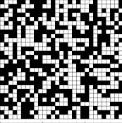
Figure 3.  : The black squares denote + domains and the white squares denote $-$ domains in a simulation with $p=0.5$ on a two-dimensional square lattice. Neither the + nor the $-$ domains percolate in this case and the domain walls, which are the boundaries between black and white squares are all finite.

One expects the same problems to arise in the lattice based study of strings and monopoles. In fact, the study of domain walls is fundamental to understanding strings and monopoles since strings, for example, may be viewed as the intersection of two types of domain walls - one on which the real part of a complex scalar field vanishes and the other on which the imaginary part vanishes [5]. If the two types of domain walls are all finite, the strings will also be finite. Hence it is suitable to first understand the percolation of domain walls.

1.2 Lattice-Free Simulations

First-order phase transitions proceed by the nucleation of bubbles of the low temperature phase in a background of the high temperature phase. The bubbles then grow, collide, and coalesce, eventually filling space with the low temperature phase. In a variety of circumstances, the low temperature phase is not unique. Here we will mainly consider the case where there are two low temperature phases, which we call plus ($+$) and minus ($-$). Our goal is to determine the percolation probability, $p_{c}$. If $p_{c}$ is found to be less than 0.5, then a range of $p$ exists for which both the $+$ and $-$ phases will percolate and, in this case, infinite domain walls will be formed [6].

Random bubble lattice

Let us begin by studying the structure of the random bubble lattice that is produced during a first order phase transition and later discuss percolation on this lattice. We write the bubble nucleation rate per unit volume as $\Gamma$, and we assume that the bubble walls expand at constant speed $v$. From these quantities we can define a length scale $\xi$ and a time scale $\tau$ by:

$$\xi=\biggr{(}{v\over\Gamma}\biggr{)}^{1/4}~{},\ \ \tau={1\over{(v^{3}\Gamma)^{1/4}}}~{},$$ (4)

where the exponents have been shown for bubbles in three dimensions. By rescaling all lengths (such as bubble radii) and all times by $\xi$ and $\tau$ respectively, the dependence of the problem on $\Gamma$ and $v$ is eliminated. Therefore dimensionful quantities such as the number density of bubbles of a given size can be rescaled to a universal distribution, and dimensionless quantities, such as the the critical percolation probability, will be independent of $\Gamma$ and $v$.

The scaling argument given above relies on the absence of any other length or time scales in the problem. Potentially such a scale is provided by $R_{0}$, the size of bubbles at nucleation, and our assumption is that $R_{0}<<\xi$. Also, note that we have taken all bubbles to expand at the same velocity $v$. This is justified if the low temperature phases within the bubbles are degenerate. If this degeneracy is lifted, different bubbles can expand at different velocities and this may result in lattices with varying properties. We are primarily interested in the exactly degenerate case which is relevant to the formation of topological defects.

In [7], the nucleation and growth of bubbles leading to the completion of the phase transition was simulated according to the scheme described in Ref. [8]. There are two ways to view this scheme. The first is a dynamic view where, as time proceeds, the number of nucleation sites are chosen from a Poisson distribution, bubbles keep growing and colliding until they fill space. The second equivalent viewpoint is static and more convenient for simulations. A certain number of spheres whose centers and radii are drawn from uniform distributions are placed in the simulation box. This corresponds to a snapshot of the bubble distribution. If the number of spheres that are laid down is large, they will fill space and the snapshot would be at a time after the phase transition has completed.

It is worth comparing the present model with currently existing models of froth. The main distinguishing feature is that the bubbles continue to grow even after they collide. This is in sharp distinction with the models used in crystal growth such as the Voronoi and the Johnson-Mehl models. In these models, crystals nucleate randomly inside a volume, grow and then, once they meet a neighboring crystal, stop growing in the direction of that neighbor. (In the Voronoi model, all crystals are nucleated at one instant while in the Johnson-Mehl model, they can nucleate at different times.) This difference between the phase transition model and the Voronoi type models is significant and the resulting lattices have different properties. Another model considered in the literature is called a “Laguerre froth”. Here the snapshot of the domains corresponds to a horizontal slice of a mountain range in which each mountain is a paraboloid. The circles of intersection of the plane and the paraboloids define the Laguerre froth [9]. In terms of bubbles, this means that the bubble walls move with a velocity that is proportional to $\sqrt{t-t_{0}}$ where $t-t_{0}$ is the time elapsed since nucleation. Such a model in two dimensions was studied by numerical methods in Ref. [10]. If the paraboloids are replaced by cones, the model comes closer to the present one.

A feature of our model of the first order phase transition is that bubbles cannot nucleate within pre-existing bubbles. This is appropriate to the case where the phases existing within bubbles are degenerate or nearly degenerate. However, in cases where a variety of non-degenerate bubbles can exist (for example, if the system has metastable vacuua), this assumption may have to be relaxed [11].

A two dimensional (dual) bubble lattice is constructed by connecting the centers of bubbles that have collided (Fig. 4). The three dimensional bubble lattice is similarly constructed and is shown in Fig. 5. The bubble lattice is almost fully triangulated though some violations of triangulation can occur. For example, if a tiny bubble gets surrounded by two large bubbles, the center of the tiny bubble will only be connected to the centers of the two surrounding bubbles and this can lead to plaquettes on the lattice that are not triangular. The characteristics of this bubble lattice hold the key to the percolation of phases and the formation of topological defects. In particular, the average number of vertices to which any vertex is connected is expected to play a crucial role. This number is called the “mean coordination number” of the lattice, and we now determine this quantity analytically.

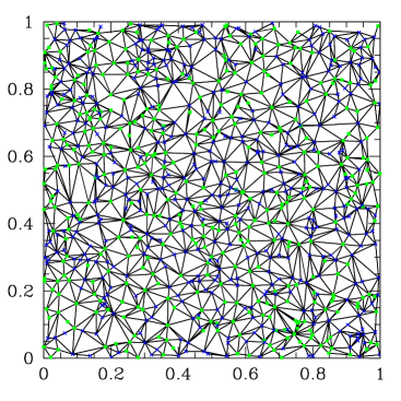
Figure 4.  : The crosses denote bubble centers that are in the + phase and the filled squares denote bubble centers that are in the - phase. If two bubbles collide, their centers are joined by straight lines. The figure then shows the “random bubble lattice” expected in a first order phase transition in two spatial dimensions.

Figure 5.  : A portion of the three dimensional dual bubble lattice.

First we consider the two dimensional case. We denote the number of points in the lattice by $P$, the number of edges by $E$ and the number of faces by $F$. Then the Euler-Poincaré formula [12] tells us

$$\chi=P-E+F$$ (5)

where, $\chi$ is the Euler character of the lattice and is related to the number of holes in the lattice (genus). In our case, the lattice covers a plane which we can compactify in some way, say by imposing periodic boundary conditions. Then $\chi$ is the genus of the compact two dimensional surface. For us it will only be important that $\chi=O(1)$. Next, if ${\bar{z}}$ is the (average) coordination number, we can see that

$$E={{\bar{z}}\over 2}P~{},$$

since, a given point is connected to ${\bar{z}}$ other points but each edge is bounded by two points. Also,

$$F={2\over 3}E~{},$$

since each line separates 2 faces but then each face is bounded by 3 lines. Now, using (5) gives

$$1-{{\bar{z}}\over 2}+{{\bar{z}}\over 3}={\chi\over P}\simeq 0~{},$$

since $P$ is assumed to be very large. Therefore, in two dimensions, ${\bar{z}}=6$, a result that first appeared in the botanical literature [13, 9].

In three dimensions the analysis to evaluate ${\bar{z}}$ is somewhat more complicated. The Euler-Poincaré formula now says

$$\chi=P-E+F-V~{},$$ (6)

where $V$ is the number of volumes in the lattice. Now, in addition to the usual coordination number ${\bar{z}}$, we also need to define a “mean face coordination number” ${\bar{y}}$ which counts the average number of faces sharing a common edge. In terms of ${\bar{y}}$ and ${\bar{z}}$, the relations between the various quantities for a triangulated three dimensional lattice are:

$$E={{\bar{z}}\over 2}P~{},\ \ F={{\bar{y}}\over 3}E~{},\ \ V={2\over 4}F~{},$$ (7)

where the first equation is as in two dimensions, the second equation follows from the definition of ${\bar{y}}$ and the fact that the lattice is triangulated, and the last relation follows because a face separates two volumes and a volume is bounded by four faces that form a tetrahedron. Inserting these relations in (6) leads to:

$${\bar{z}}={{12}\over{6-{\bar{y}}}}~{},$$ (8)

where, as before, we assume that $P$ is very large and ignore the $\chi/P$ term. Note that the relation between ${\bar{y}}$ and ${\bar{z}}$ is purely topological and will hold for any triangulated lattice.

We now want to estimate ${\bar{y}}$. For this we work in a “mean field” approximation where we assume that the edge lengths are fixed. We consider two vertices $A$ and $B$ separated by a unit distance. We wish to find the number of points that can be connected to both $A$ and $B$, subject to the constraint that the connected points are at unit distance from each other. This will give the (average) number of faces that share the edge from $A$ to $B$ and hence will be the face coordination number ${\bar{y}}$. Let us choose $A$ to be at the center of a sphere of unit radius and $B$ to be at the North pole. Then the additional points $P_{1}$,…,$P_{y}$, have to lie on the circle at latitude 60 degrees to satisfy the distance constraint. Then one finds that the azimuthal angular separation of two sequential points $P_{i}$ and $P_{i+1}$ is 70.5 degrees. Therefore

$${\bar{y}}={{360}\over{70.5}}=5.1,$$ (9)

which then leads to [14]

$${\bar{z}}=13.4~{}.$$ (10)

It is worth noting the ingredients that have entered into the analytic estimate of ${\bar{z}}$. The relation (8) is a topological statement about the lattice, but the estimate for ${\bar{y}}$ is geometric, depending on the assumption that the edges have fixed length. In principle, the edge lengths can fluctuate but our estimate for ${\bar{y}}$ will still be valid if the fluctuations average out.

In Fig. 6 we show the distribution of coordination number in our three dimensional simulations. The average coordination number is found to be ${\bar{z}}=13.34\pm 0.05$ and agrees quite closely with the mean field result. For comparison, Voronoi foam has ${\bar{z}}=15.54$ and the Johnson-Mehl model has ${\bar{z}}>13.28$ [15]. The reason why ${\bar{z}}$ is larger in the Voronoi model is that, in this model, the cells stop growing on collision in the direction of the collision, thus leading to anisotropic growth. It can be shown that anisotropy of the cells leads to a higher value of ${\bar{z}}$ [9].

Figure 6.  : The coordination number relative frequency distribution for the three dimensional dual bubble lattice.

The mean value of $z$ is not a good characteristic of the distribution of $z$ since the distribution is skewed (the modal value of $z$ is 7) and it is of interest to characterize the entire distribution of $z$. In the literature on domain physics, attempts to derive the distribution of coordination number are often based on maximizing the “entropy” of the lattice. The expression used for the entropy is the one proposed by Shannon [16, 17].

$$S=-\sum_{n}p_{n}\ln p_{n}$$ (11)

where, $p_{n}$ is the probability that a vertex will be connected to $n$ other vertices. In addition, one needs to insert the Euler-Poincaré constraint in the Shannon entropy via Lagrange multipliers. (There is also the issue of assigning a priori probabilities [17].) In two dimensions the constrained extremization is relatively straightforward, since the Euler-Poincaré constraint fixes the average coordination to be 6, i.e.

$$\sum_{n}np_{n}=6\ \ ({\rm in\ 2D})\ .$$

In three dimensions, we may once again introduce the constraint that the average coordination number of the lattice is fixed (even though there is some freedom in choosing its value). Then, on extremizing $S$ in eq. (11) with respect to $p_{n}$, we find an exponential fall-off of the distribution. Indeed, the distribution shown in Fig. 6 has an exponential fall-off:

$$f(z)\sim\exp[-0.25z]\ ,\ \ z>20\ .$$ (12)

Percolation on a random bubble lattice

We now turn to the formation of defects on the bubble lattice. We put a + phase on a bubble with probability $p$ and a $-$ phase with probability $1-p$ (as shown in Fig. 4 in the two dimensional case). We then find the size distribution of + clusters and calculate the moments of the cluster distribution function after removing the largest cluster from the distribution [18]. That is, we calculate:

$$S_{l}(p)=\sum_{s\neq s_{max}}s^{l}n_{s}(p)$$ (13)

for $l=0,1,2,...$, where the sum is over cluster sizes ($s$) but does not include the largest cluster size, and $n_{s}(p)$ is the number of clusters of size $s$ divided by the total number of bubbles. In Fig. 7 we show the first three moments as a function of $p$, where the turning point in $S_{2}$ marks the onset of percolation. To understand this, first consider the behavior of the second moment for small $p$. As we increase $p$, there are fewer + clusters (as seen from the $S_{0}$ graph) probably due to mergers, but the merged cluster sizes are bigger (as seen from the $S_{1}$ graph). Since the second moment places greater weight on the size of the cluster than on the number density as compared to the lower moments, it grows for small $p$. For large $p$, however, as we increase $p$ further, the additional + clusters join the largest cluster of +’s and are not counted in the second moment. In fact, some of the smaller clusters also merge with the largest cluster and get removed from the sum in (13). This causes the second moment to decrease at large $p$. Hence, the second moment has a turning point and the location of this turning point at $p_{c}$ marks the onset of percolation. In three dimensions we find $p_{c}=0.17\pm 0.01$ (from Fig. 7), which is well under 0.5, while in two dimensions we find $p_{c}=0.50\pm 0.01$ which is consistent with 0.50. (The two dimensional version of Fig. 7 may be found in [6].)

It is interesting to compare the critical probabilities we have found with lattice based results for site percolation where the regular lattice has a coordination number close to that of the random bubble lattice. In two dimensions a triangular lattice has ${\bar{z}}=6$ and $p_{c}=0.5$. In three dimensions, a face centered cubic lattice has ${\bar{z}}=12$ and $p_{c}=0.198$ [18]. These values of the critical probabilities are fairly close to our numerical results.

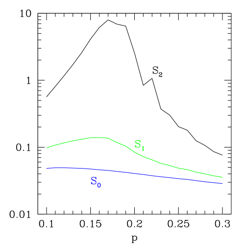
Figure 7.  : The zeroth, first and second moments of the cluster distribution function versus the probability $p$ in three dimensions.

Open Problems

Exponents: The value of the critical percolation probability is not universal. However, the percolation exponents are expected to be universal. These have not been evaluated for the random lattice and would be worth determining.

Bias: The rather low value of $p_{c}$ in three dimensions means that domain walls formed between degenerate vacua ($p=0.5$) will percolate and almost all of the wall energy will be in one infinite wall. Furthermore, even if the vacua are not degenerate, i.e. there is bias in the system, infinite domain walls can still be produced. If the properties of the bubble lattice are insensitive to small biases, infinite domain walls would be produced for $p>0.17$. However, it is likely that the bubble lattice will depend on the bias in three ways. First, the nucleation rate of bubbles of the metastable vacuum will be suppressed compared to that of the true vacuum. Secondly, the velocity with which bubbles of the two phases grow can be different. Thirdly, bubbles of the true vacuum may nucleate within the metastable vacuum. In addition to these factors, bubbles may not retain their spherical shape while expanding due to instabilities in their growth. The effect of these factors on the percolation probability will be model dependent. For example, the bubble velocities will depend on the ambient plasma, and the nucleation rates on the action of the instantons between the different vacuua. The effect of including these factors on the random bubble lattice and percolation has not yet been studied.

Other defects: The formation of topological strings on the random bubble lattice follows the algorithm described in Ref. [1]. It is found that about 85% of the strings in the simulation are infinite. This number should be compared with earlier static simulations of string formation which yield a slightly lower fraction (about $80\%$). The distribution of other types of defects should be determined.

Phase equilibration: The analysis described here neglects phase equilibration processes when domains of different phases collide. This may be justified if the time scale $\tau$ in eq. (4) is short compared to the typical time required for phase equilibration. In the case of domain walls, phase equilibration in two colliding bubbles can only occur by the motion of the phase separating wall across the volume of one of the bubbles. In this case, the neglect of phase equilibration is justified if the domain wall velocity is much smaller than the bubble wall velocity. It would be interesting to see how the results change if phase equilibration is important.

2 Interactions of Defects

Once a string network forms in any system, the strings start moving under their tension. Inevitably string collisions occur. What happens then?

It is a classic result that two strings intercommute (reconnect) upon intersection (Fig. 8). This conclusion seems to hold regardless of the details of the collision (angles and velocities), as well as the physical model (global or local strings). Intercommuting has been observed in computer simulations and experimentally. There are important supporting arguments that provide insight into intercommuting but there is no analytical proof that intercommuting of Abelian strings must necessarily occur.

Figure 8.  : Two incoming strings in (a) collide, reconnect and emerge as in (b).

The phenomenon of intercommuting is vital to the relaxation (coarsening) of the system. In cosmology, intercommuting provides a means for the string network to dissipate and prevent it from dominating the universe.

A question that has recently attracted some attention is the interaction of different types of defects arising in the same physical model [20]. Consider, for example, a phase transition in which both domain walls and point defects (global or local monopoles) can be formed. On formation, the domain walls will start moving under their own tension. Inevitably, they will collide with the point defects. What happens then? Do the point defects pass through the walls to the other side? Or do they undergo some microphysical transformation? The answer to these questions are very important for understanding the coarsening of the system.

Based on several different arguments, it was suggested in [20] that the monopoles do not pass through the domain walls. Instead they undergo a microphysical transformation and unwind on the walls. The arguments in support of this conjecture are:

(i) There is an attractive force between the monopoles and the walls since monopoles can save the expense of having to go off the vacuum in their core by moving on to the wall. So the monopoles can form bound states with the walls. Then, as there is no topological obstruction to the unwinding of monopoles on the wall, the monopoles on the wall can continuously relax into the vacuum state.

(ii) The investigation of a similar system - Skyrmions and walls - has been dealt with in full detail in Ref. [21]. These authors find that the Skyrmion hits the wall, sets up traveling waves on the wall and dissipates. They also find that, even though it is topologically possible for the Skyrmion to penetrate and pass through the domain wall, this never happens. They attribute their finding to the coherence required for producing a Skyrmion. That is, the penetration of a Skyrmion may be viewed as the annihilation of the incoming Skyrmion on the wall and the subsequent creation of a Skyrmion on the other side. However, the annihilation results in traveling waves along the wall that carry off a bit of the coherence required to produce a Skyrmion on the other side. Hence, even though there is enough energy in the vicinity of the collision, a Skyrmion is unable to be created on the other side of the wall. I think that these considerations apply equally well to monopole-wall interactions and that monopoles will never pass through the wall - just as strings never pass through each other.

(iii) The interactions of vortices and domain walls separating the A and B phases of ³He have been studied and also observed experimentally. It is found that singular vortices do not penetrate from the B phase into the A phase [22].

What is sorely needed is a direct check of this conjecture. (A very recent study [23] has confirmed monopole dissolution on walls in a particular model under some restricted conditions.) If confirmed, it would be good to be able to understand the result at a deeper level.

Figure 9.  : The figure on the left shows the projected string configuration along with the randomly located unlensed sources inside the dashed box. The figure on the right shows the resulting images of the sources The full string shown in the figure on the left was used to determine the lensing effects.

3 Observation of Cosmic Strings

If cosmic strings lie between us and some distant sources of light, they will cause distortions in the image of the source or cause multiple images to be produced. Two of the most distant cosmological sources are the cosmic microwave background radiation and quasars. The cosmic microwave background radiation comes to us from when the universe was only about a million years old, while the light from quasars started out about 1 billion years ago. (The present age of the universe is about 10 billion years.) A major difference between these two sources is that the CMBR is an almost uniform source, while the quasars are point-like. This leads to different kinds of observable signatures of strings in the two cases. Cosmic strings can imprint a pattern of anisotropy of the CMBR and they can gravitationally lens quasars and galaxies with a frequency given by the probability that a quasar will lie behind a string. Both effects are quite small - the anisotropy is at the level of about 1 part in $10^{5}$ and the probability of lensing is also of this order of magnitude. In either case, however, the signature of strings appears to be quite distinct and can lead to confirmation of their presence or absence at a certain energy scale.

3.1 Gravitational lensing

The most tricky part in studying the gravitational lensing of distant sources by strings is the actual construction of the string itself. In Ref. [24], the string was constructed by using flat spacetime simulations as proposed by Smith and Vilenkin [25]. Light from distant sources is then propagated in the gravitational field of this string. The results are shown in Fig. 9.

What seems most striking about the lensed sources is that they seem to trace out the string. This is due to the wiggly nature of the string since small sections of the projected string can act like very massive objects.

Figure 10.  : The graph on the left shows the total angular power spectrum in CMBR anisotropy for wiggly (solid line) and smooth (dashed line) strings when $\Omega_{baryons}=.05$, $\Omega_{CDM}=0.25$ and $\Omega_{\Lambda}=0.7$ and using small values for the string velocities. The graph on the right shows the power spectrum of the density inhomogeneities for the same two models and the observed data points.

3.2 CMBR distortions

Once again, the most difficult aspect of calculating the CMBR distortions is to find a reliable model of the network of strings. Direct simulations of the string network have provided invaluable information about certain properties of the network. The game is to convert this information into a model that can then be fed into the machinery to calculate the CMBR anisotropy. Recently I have been working with Levon Pogosian to compute the anisotropy using the model developed in [26, 27]. (Some other references to related literature may be found in [28].) The results depend on details of the string model as well as the cosmological model. In Fig. 10 I show our preliminary results for the power in the $l^{th}$ spherical harmonic of the CMBR anisotropy as a function of $l$ together with the observed data points. (Space does not permit a lengthier explanation of the graphs in this section but background details can be found in several textbooks, for example Ref. [29].) At the moment, the observations do not confirm or reject the hypothesis that cosmic strings may be responsible for the CMBR anisotropy.

The density perturbations produced by cosmic strings would lead to large-scale structure formation. Then one might compare the power spectrum of the density inhomogeneities produced by strings to those observed in the galaxy distribution. Here too, the details of the string and the cosmological model are all crucial. Within the limitations of the models used, the string predictions do not agree with observations at the level of a factor of about 2 in the amplitude of the density fluctuations (Fig. 10). However, further modeling of the string network and analysis is necessary before we can be sure of this result.

Acknowledgments

This work was supported by the Department of Energy (USA).

References

- [1] T. Vachaspati and A. Vilenkin, Phys. Rev. D30, 2036 (1984).
- [2] R. J. Scherrer and J. Frieman, Phys. Rev. D33, 3556 (1986).
- [3] E. J. Copeland, T. W. B. Kibble and D. A. Steer, Phys. Rev. D58, 043508 (1998).
- [4] L. Pogosian and T. Vachaspati, Phys. Lett. B423, 45 (1997).
- [5] R. J. Scherrer and A. Vilenkin, Phys. Rev. D56, 647 (1997); Phys. Rev. D58 103501 (1998).
- [6] T. Vachaspati, ICTP 1997 Summer School Lectures on Cosmology, hep-ph/9710292 (1997).
- [7] A. A. de Laix and T. Vachaspati, Phys. Rev. D59 045017 (1999).
- [8] J. Borrill, T. W. B. Kibble, T. Vachaspati and A. Vilenkin, Phys. Rev. D52, 1934 (1995).
- [9] See the contribution by N. Rivier in “Disorder and Granular Media”, eds. D. Bideau and A. Hansen (North-Holland, 1993).
- [10] H. Telley, Ph. D. Thesis, EPFL, Lausanne, 1989 (unpublished).
- [11] M. Gleiser, A. F. Heckeler and E. W. Kolb, Phys. Lett. B405, 121 (1997).
- [12] C. Nash and S. Sen, “Topology and Geometry for Physicists”, Academic Press, London (1983).
- [13] F. T. Lewis, Anat. Record 38, 341 (1928); ibid. 50, 235 (1931).
- [14] H. S. M. Coxeter, Ill. J. Math. 2, 746 (1958); J. A. Dodds, J. Coll. Interf. Sci. 77, 317 (1980); N. Rivier, J. Physique Coll. 43, C9-91 (1982).
- [15] J. L. Meijring, Philips Res. Rep. 8, 270 (1953).
- [16] C. E. Shannon, Bell Systems Technical Journal 27, 379 (1948); reprinted in C. E. Shannon and W. Weaver, “The Mathematical Theory of Communication”, (University of Illinois Press, 1949).
- [17] N. Rivier, Phil. Mag. B52, 795 (1985).
- [18] D. Stauffer, Phys. Rep. 54, 1 (1979).
- [19] L. M. A. Bettencourt and T. W. B. Kibble, Phys. Lett. B332, 297 (1994).
- [20] G. Dvali, H. Liu and T. Vachaspati, Phys. Rev. Lett. 80, 2281 (1998).
- [21] A. Kudryavtsev, B. Piette, W. J. Zakrzewski, hep-th/9709187, DTP-97/25 (1997).
- [22] H.-R. Trebin and R. Kutka, J. Phys. A28, 2005 (1995); T. Sh. Misirpashaev, Sov. Phys. JETP 72, 973 (1991); M. Krusius, E.V. Thuneberg and U. Parts, Physica B197, 376 (1994).
- [23] S. Alexander, R. Brandenberger, R. Easther and A. Sornborger, hep-ph/9903254 (1999).
- [24] A. A. de Laix, L. M. Krauss and T. Vachaspati, Phys. Rev. Lett. 79, 1968 (1997).
- [25] A. G. Smith and A. Vilenkin, Phys. Rev. D36, 990 (1987).
- [26] G. Vincent, M. Hindmarsh and M. Sakellariadou, Phys. Rev. D55, 573 (1997).
- [27] A. Albrecht, R. Battye and J. Robinson, Phys. Rev. Lett., 79, 4736 (1997); Phys. Rev. D59, 023508 (1998).
- [28] D.P. Bennet, F.R. Bouchet and A. Stebbins, Nature 335 410, (1988); L. Perivolaropoulos, Phys. Lett. B298, 305 (1993); L. Perivolaropoulos, Ap. J. 451, 429 (1995); B. Allen, R. R. Caldwell, S. Dodelson, L. Knox, E. P. S. Shellard and A. Stebbins, Phys. Rev. Lett. 79, 2624 (1997); U-L. Pen, U. Seljak and N. Turok, Phys. Rev. Lett. 79, 1611 (1997); P.P. Avelino, E.P.S. Shellard, J.H.P. Wu and B. Allen, Phys. Rev. Lett. 81, 2008 (1998); R. Battye, J. Robinson and A. Albrecht, Phys. Rev. Lett. 80, 4847 (1998); C. Contaldi, M. Hindmarsh and J. Magueijo, Phys. Rev. Lett. 82, 679 (1999); E.J. Copeland, J. Magueijo and D.A. Steer, astro-ph/9903174.
- [29] “Cosmological Physics”, J. A. Peacock, Cambridge University Press (1999).