Spallative Nucleosynthesis in Supernova Remnants

Abstract

We calculate the spallative production of light elements associated with the explosion of an isolated supernova in the interstellar medium, using a time-dependent model taking into account the dilution of the ejected enriched material and the adiabatic energy losses. We first derive the injection function of energetic particles (EPs) accelerated at both the forward and the reverse shock, as a function of time. Then we calculate the Be yields obtained in both cases and compare them to the value implied by the observational data for metal-poor stars in the halo of our Galaxy, using both O and Fe data. We find that none of the processes investigated here can account for the amount of Be found in these stars, which confirms the analytical results of Parizot and Drury (1999). We finally analyze the consequences of these results for Galactic chemical evolution, and suggest that a model involving superbubbles might alleviate the energetics problem in a quite natural way.

1 Introduction

The class of light elements, namely Li, Be and B, sets itself apart from any other by its interstellar origin (except for part of the ⁷Li, produced in the Big Bang ages, and perhaps part of the ¹¹B, produced in supernova (SN) explosions by neutrino-spallation). Concentrating on the most representative isotope, the abundance of ⁹Be in stars of increasing metallicity can be regarded as the witness and tracer of the nuclear spallation efficiency during Galactic chemical evolution. Indeed, virtually every atom of Be observed in the atmosphere of stars must have been produced by the spallation of a larger nucleus, most probably C or O, induced by the interaction of energetic particles (EPs) with the interstellar medium (ISM).

Since the first measurement of Be in a very metal-poor star at the beginning of the decade (Gilmore et al. 1991), increasing evidence has been gathered showing that the abundance of Be and B in the early Galaxy (until the ambient metallicity is 10% that of the sun, say) kept increasing jointly and linearly with ordinary metallicity tracers, such as Fe or O, as if they were actually primary elements (Duncan et al. 1992,1997; Edvardsson et al. 1994; Gilmore et al. 1992; Kiselman & Carlsson 1996; Molaro et al. 1997; Ryan et al. 1994). Now they are not, since as we just recalled C and O nuclei have to be produced first in order that they can be spalled by EPs into light elements. The observations therefore suggest that some process must act to ensure that, on average, an equal amount of Be is synthesized each time a given mass of Fe or O is ejected into the ISM. It should be clear, however, that this statement relies on the assumption that the abundances of O and Fe are proportional to one another, at least during the early evolution stages in which we are interested here.

This assumption has long been used with high confidence level based on both theoretical and observational arguments, but new observations seem to contradict it dramatically (Israelian et al. 1998; Boesgaard et al. 1998). Although an independent confirmation of these observations would be welcome, they have recently been used to reappraise the alleged ‘primary behavior’ of ⁶LiBeB Galactic evolution (Fields and Olive, 1999). Indeed, if the O/Fe abundance ratio is not constant but actually decreases with metallicity, then the observed approximate constancy of the Be/Fe ratio implies an increasing Be/O ratio. Fields and Olive (1999) find a Be–O logarithmic slope in the range 1.3–1.8, which seems to contradict both the primary scenario (slope 1) and the secondary scenario (slope 2), in which the spallation reactions producing the light elements are induced by standard Galactic cosmic rays (GCRs) accelerated out of the ISM. However, the current lack of Be and O abundance measurements in the same very metal-poor stars (with [O/H] $=10^{-3}$, say) makes the data marginally compatible, within error bars, with both scenarii.

While the situation should be soon clarified, notably by the accumulation of data at lower metallicity and independent measurements of Be, B, O and Fe in the same set of halo stars, we (Parizot and Drury, 1999; Paper I) choose to investigate the Be production in the ISM from the other direction, i.e calculate the Be yield associated with the explosion of an isolated supernova (SN) in the ISM, according to current knowledge about supernova remnant (SNR) evolution and standard shock acceleration, and compare this Be yield with the value required to explain the observed Be/Fe ratio in metal-poor stars. We identified two different mechanisms leading naturally to a primary evolution of Be in the early Galaxy. In the first mechanism, particles from the ambient ISM (i.e. metal-poor) are accelerated at the forward shock of the SN and confined within the SNR until the end of the Sedov-like evolution phase. There, they interact with the freshly synthesized C and O nuclei, and therefore produce Be by spallation at a much higher rate than in the (secondary) GCR nucleosynthesis scenario in which they merely interact with the ambient, metal-poor ISM. In the second mechanism, particles from the enriched SN ejecta are accelerated at the reverse shock and again confined within the SNR during Sedov-like phase, where they suffer adiabatic losses through which they lose between 30% and 70% of their initial energy, depending on the ambient density. After the end of the Sedov-like phase, these particles diffuse out in the ISM where the energetic C and O nuclei can be spalled by the H and He atoms at rest in the Galaxy.

We have shown in Paper I, through approximate analytical calculations, that the total Be yield obtained by processes 1 and 2 depends on the ambient density, and that this third mechanism is actually the most efficient (for light element production) in most cases, though not efficient enough to account for the observed Be/Fe ratio of $\sim 1.6\,10^{-6}$. If each SN ejects on average 0.1 $M_{\odot}$ of Fe in the ISM, then the average Be yield per SN must be $\sim 4\,10^{48}$ atoms (cf. Ramaty et al. 1997), which exceeds even our most optimistic calculated yields by about one order of magnitude. We concluded that another mechanism or source of energy should be invoked, and argued that a model based on superbubble acceleration (involving the collective effect of SNe rather than individual SN shock acceleration) is a quite natural and promising candidate. In this paper, we confirm the results of Paper I by performing time-dependent numerical calculations, and discuss in more details their implications for Galactic chemical evolution scenarii. The reader is referred to Paper I for a more detailed description of the mechanisms considered here, and a discussion of their motivation and theoretical justification.

2 Why we need to do time-dependent calculations

We intend to calculate the Li, Be and B (LiBeB) production induced by the interaction of energetic particles within a SNR. We shall first consider the fate of the particles accelerated out of the ambient, zero metallicity ISM entering the forward shock created by a SN explosion (process 1), and then turn to the acceleration of particles from the SN ejecta at the reverse shock, on a very short time scale around the so-called sweep-up time, ${t_{\rm SW}}$ (process 2). It turns out that both of these processes are highly non-stationary, for a number of reasons which we now review.

2.1 EPs accelerated at the forward shock

Considering first process 1, we expect that the particle injection power be more or less proportional to the power of the shock, which is a decreasing function of time as the SNR evolves. Therefore the injection rate of the EPs is not constant, and no steady-state distribution function of the EPs within the SNR is ever reached. If everything else was constant in the problem, we could however calculate the total energy injected in the form of EPs during the whole process, and multiply it by the steady-state spallation efficiency (defined as the ‘number of nuclei synthesized per erg injected’), evaluated from standard steady-state calculations. This would provide us with the total spallation yields (i.e. the time integral of the spallation rates), which are the only observationally relevant quantities. This, however, cannot be done in the case we are considering, because the chemical composition of the target, namely the interior of the SNR, is also evolving during the expansion.

Indeed, as more and more metal-poor material is swept-up from the ISM by the shock, the metal-rich SN ejecta suffer stronger and stronger dilution, which makes the spallation of C and O less and less efficient. As a consequence, even though we can evaluate the total energy eventually imparted to EPs, we cannot deduce the spallation yields from it because we don’t know what composition to choose for the target. Again, if this was the only non stationary feature in the process, we could still calculate the average target composition and compute the spallation yields from it. But since both the EP injection rate and the target composition are functions of time, steady-state models cannot be used in any consistent way, and a fully time-dependent calculation is required.

Qualitatively, it is easy to show that the yields which we obtain by integrating the time-dependent spallation rates must be appreciably higher than those derived from steady-state estimates using the total energy injected in the form of EPs and the (constant) mean target composition. Indeed, the latter amounts to assuming that the injection rate is also constant and equal to the average power of the EPs (i.e. the total energy divided by the duration of the process). However, in the time-dependent model, we take advantage of the fact that the EP power is higher at the beginning, when the target composition is richer in C and O. In other words, the spallation efficiency is higher when the EP fluxes are higher too, and conversely, less energy is imparted to the less efficient EPs accelerated towards the end of the process.

In addition to the sources of non-stationarity just mentioned (time-dependent injection and dilution of the ejecta), we also have to take into account the adiabatic losses suffered by the EPs as they wander inside the expanding volume of the SNR. Now these adiabatic losses are essentially function of time, becoming smaller and smaller as the SNR expands and the shock velocity gets lower. This again can only be taken into account in a time-dependent model.

2.2 EPs accelerated at the reverse shock

Coming now to the case of process 2, where particles from the enriched material ejected by the supernova are accelerated at the reverse shock, it is clear that the dilution effect mentioned above does not have any significant influence anymore. Indeed, the light element production is now dominated by the spallation of energetic C and O nuclei interacting with ambient H and He, instead of ambient C and O interacting with energetic H and He nuclei in the case of process 1 (see Figs. 1 and 4). The abundance of (non energetic) C and O in the target has therefore only a negligible influence, since these nuclei hardly contribute to the spallation yields. Nevertheless, the time dependence of the EP injection and the adiabatic losses still have to be taken into account, which is enough to make time-dependent calculations indispensable.

As has been argued in Paper I, the curve representing the power in the reverse shock, $\mathcal{P}_{\mathrm{in}}$, as a function of time strongly peaks around the sweep-up time, ${t_{\rm SW}}$, which is defined as usual as the time at which the swept-up mass is equal to the ejected mass. This also approximately marks the end of the free expansion phase and the beginning of the adiabatic (or Sedov-like) phase. In the absence of a motivated prescription for the reverse shock power function, $\mathcal{P}_{\mathrm{in}}(t)$, and on the understanding that its time scale is short as compared to the energy loss time scale, we shall consider below the injection of EPs as instantaneous in the case of process 2. We thus just could not be further away from a steady-state. However, as above, were this the only non-stationary feature of the process, we could still obtain the integrated spallation yields from steady-state calculations by merely multiplying the total energy injected in the form of EPs by the spallation efficiency, which in this case is almost independent of the target composition. Unfortunately, as already indicated, the adiabatic losses are also a function of time, and will therefore cause the aforementioned spallation efficiency to vary as the process goes on.

On the other hand, once the EPs leave the SNR at the end of the Sedov-like phase to interact with the surrounding ISM, they will only suffer the usual Coulombian losses, which are essentially independent of time. The above argument therefore does not apply anymore and this final part of process 2 (occuring outside the remnant) could be worked out with purely steady-state machinery. This is in fact what we did in Paper I (see its Sect. 4), in our study of what we then called process 3. Here, however, we shall not distinguish between the part of the process occuring inside the SNR, and the part occuring outside (former process 3), because our time-dependent numerical model allows us to treat both on the same footing. In particular, we obtain in this way not only the total LiBeB yields, but also their production rates as a function of time, whose time integral can be sucessfully checked to be equal to the steady-state yields.

3 Description of the theoretical and numerical model

It has been shown in the previous section that the spallative production of light elements associated with the explosion of a SN in the ISM is essentially a dynamical process, and therefore requires non-stationary calculations. A general time-dependent model for the interaction of EPs in the ISM has been developed and presented in Parizot (1999), so we shall use it here extensively, recalling only the results relevant to our specific problem and calculating the required inputs for processes 1 and 2.

3.1 The mathematical formalism and the physical ingredients

In each case, we separate the acceleration of the energetic particles (EPs) from their propagation and interaction within the SNR. This is legitimate because the time scale for acceleration up to the energies we are concerned with is very much smaller than any other time scale in the problem, whether dynamical (SNR evolution) or physical (energy loss rate, spallation rates). Consequently, our calculations apply to the EPs once they have been ‘injected’ inside the SNR (from the region close to the shock). Let us assume for the moment that we have determined the so-called injection function, $Q_{i}(E,t)$, which we define as the number of particles of species $i$ introduced at energy $E$ and time $t$, per unit energy and time (in $(\mathrm{MeV/n})^{-1}\mathrm{s}^{-1}$). The EP distribution function, $N_{i}(E,t)$ then satisfies the usual propagation equation (see Parizot 1999) :

$$\begin{split}\frac{\partial}{\partial t}N_{i}(E,t)&+\frac{\partial}{\partial E}(\dot{E}_{i}(E)N_{i}(E,t))\\ &=Q_{i}(E,t)+Q_{i}^{\prime}(E,t)-\frac{N_{i}(E,t)}{\tau_{i}^{\mathrm{tot}}(E)},\end{split}$$ (1)

where $\dot{E}_{i}(E)$ is the energy loss rate for the nuclei of species $i$ at energy $E$ (in $(\mathrm{MeV/n})\mathrm{s}^{-1}$), $Q_{i}^{\prime}(E,t)$ is the production rate of nuclei $i$ as secondary particles, and $\tau_{i}^{\mathrm{tot}}(E)$ is the time scale for catastrophic losses, such as nuclear destruction or escape from the region under study.

Since we are concerned with spallation reactions involving the nuclei of the CNO group, we can neglect the two-step processes such as ${}^{16}\mathrm{O}+\mathrm{p}\rightarrow$ ${}^{12}\mathrm{C}$ followed by ${}^{12}\mathrm{C}+\mathrm{p}\rightarrow$ ${}^{9}\mathrm{Be}$. We indeed found, using a steady-state model, that the omission of the two-step processes leads too an error of at most $\sim 10\%$, in good agreement with Ramaty et al. (1997) calculations. Since this is smaller than the other observational and theoretical uncertainties, and their implementation in a time-dependent model greatly complicates the situation, we shall neglect them here (Note that in any case, even if there were no other uncertainty in the problem, it is much more accurate to do time-dependent calculations without two-step processes than steady-state calculations including two-step processes, as our simulations have shown). To state this in a more physical way, we can claim that the spallative production of carbon amounts to at most a few percents of the initial CNO supply from the supernova explosion. To the level of precision of the SN models, to mention that only, this correction is of no significance, so we shall simply drop $Q_{i}^{\prime}(E,t)$ in Eq. (1).

Concerning the catastrophic loss time, $\tau_{i}^{\mathrm{tot}}$, it is obtained for stable nuclei as :

$$\frac{1}{\tau_{i}^{\mathrm{tot}}(E,t)}=\frac{1}{\tau_{i}^{\mathrm{esc}}(E,t)}+\frac{1}{\tau_{i}^{\mathrm{D}}(E,t)},$$ (2)

where $\tau_{i}^{\mathrm{esc}}$ is the escape time, and $\tau_{i}^{\mathrm{D}}$ is the destruction time. The latter is derived from semi-empirical formulas giving the total inelastic cross sections $\sigma_{i,j}$ for a projectile $i$ in a target of species $j$ (Silberberg & Tsao 1990), according to :

$$\frac{1}{\tau_{i}^{\mathrm{D}}(E,t)}=[\sum_{j}\sigma_{i,j}(E)n_{j}(t)]v(E),$$ (3)

where $v(E)$ is the velocity of the energetic particle and $n_{j}(t)$ is the number density of target species $j$ at time $t$.

Following the above qualitative analysis (see Paper I for more details), we assume that the time of escape out of the SNR is infinite during the Sedov-like phase of the SNR expansion, and ‘zero’ afterwards. This merely translates the fact that the EPs are confined within the SNR during the adiabatic phase (at least those of lowest energy, which produce most of the spallative LiBeB), and then leak out on a very short time scale. Once the EPs have escaped from the SNR, we need to distinguish between our two processes. In the first case (acceleration at the forward shock), the EPs are deprived of CNO and will not give rise to enough spallation reactions out of the SNR to raise the LiBeB production in any significant way. This is due to the very low ambient metallicity. In the second case, however, the EPs are made of the supernova ejecta themselves and are thus rich in CNO. As a consequence, as far as LiBeB production is concerned, there is no difference whether they interact within or outside the SNR, as interactions with H and He nuclei dominate anyway. We must therefore follow these accelerated nuclei after the end of the adiabatic phase, and compute the corresponding contribution to the total production of light elements.

Concerning the energy loss rate, $\dot{E}_{i}(E)$, we need to take into account both ionisation (Coulombian) and adiabatic losses. The former are very common and just cannot be avoided as soon as energetic particles are to be interacting in the ISM. The latter, however, must be included here because the EPs are confined within the SNR where their velocities are randomized. As a consequence, they do participate to the internal pressure which drives the remnant during the Sedov-like phase, and suffer the adiabatic losses like any other particle working outward when reflected at the expanding shell. Quantitatively, these adiabatic losses have been calculated in Paper I. They are given by Eq. (14) there, namely :

$$\frac{\dot{p}}{p}=-\frac{3}{4}\frac{\dot{R}}{R}\,\,,$$ (4)

where $p$ is the momentum of the particle and $R(t)$ is the radius of the shock. Assuming the Sedov-like expansion law ($R(t)\propto t^{2/5}$) and writing the loss rate in terms of energy, we obtain :

$$\dot{E}_{\mathrm{ad}}(E,t)=-\frac{3}{10}\frac{E}{t}\left(\frac{E+2m_{p}c^{2}}{E+m_{p}c^{2}}\right)$$ (5)

This energy loss rate does not depend on the EP species, but is clearly a function of time. On the other hand, the ionisation losses, $\dot{E}_{\mathrm{ion}}(E)$, do depend on the nuclear species, as well as on time, indirectly, through the density and composition of the ambient medium. Indeed, it has to be realised that the medium in which the EPs are ‘propagating’, namely the interior of the SNR, is initially very rich in freshly synthesized CNO nuclei, and then gets poorer and poorer in metals as the ejecta are being diluted in the ambient, metal-poor, swept up material.

This dilution effect is most important for the calculation of the total LiBeB production through our first mechanism (acceleration of the ISM at the forward shock). Indeed, the instantaneous production rates are directly proportional to the density of CNO within the remnant at time $t$, which goes like $R^{-3}$, i.e. $t^{-6/5}$. Quantitatively, the LiBeB production rates are obtained by integrating the spallation cross sections over the EP distribution functions :

$$\frac{\mathrm{d}N_{k}}{\mathrm{d}t}=\sum_{i,j}\int_{0}^{\infty}\mathrm{d}E^{\prime}N_{i}(E^{\prime},t)n_{j}(t)\sigma_{i,j;k}(E^{\prime})v_{i}(E^{\prime}),$$ (6)

where $\sigma_{i,j;k}$ is the cross section for the reaction $i+j\rightarrow k$, and $n_{j}$ is the number density of nuclei $j$ in the target (here, the interior of the SNR).

The total LiBeB production is then obtained for the first mechanism by integrating these production rates from ${t_{\rm SW}}$ to ${t_{\rm end}}$, which marks the end of the Sedov-like phase as well as the end of the confinement of the EPs inside the SNR. For the second mechanism, we need to integrate from $t_{\mathrm{SW}}$ to the confinement time of the cosmic rays within the Galaxy. As we shall see below, integrating up to infinity only leads to a small overestimate of the total LiBeB production, since the low energy cosmic rays responsible for most of that production have anyway a short lifetime above the spallation thresholds.

The sweep-up time, ${t_{\rm SW}}$, is obtained straightforwardly from its definition as a function of the SN parameters and the ambient number density, $n_{0}$ :

$$\hbox{${t_{\rm SW}}$}=(1.4\,10^{3}\,\mathrm{yr})\left(\frac{M_{\mathrm{ej}}}{10\hbox{$M_{\odot}$}}\right)^{\frac{5}{6}}\left(\frac{E_{\mathrm{SN}}}{10^{51}\mathrm{erg}}\right)^{-\frac{1}{2}}\left(\frac{n_{0}}{1\mathrm{cm}^{-3}}\right)^{-\frac{1}{3}}.$$ (7)

The determination of ${t_{\rm end}}$ is more difficult and somewhat arbitrary, even in the approximation of a perfectly homogeneous circumstellar medium. We argued above and in Paper 1 that ${t_{\rm end}}$ should more or less coincide with the end of the Sedov-like phase, when the shock induced by the SN explosion becomes radiative, that is when the cooling time of the post-shock gas becomes of the same order as the dynamical time. This depends on the cooling function which in turn depends on the density and metallicity of the post-shock gas. Such details and their influence on ${t_{\rm end}}$ have been considered in Paper I. Here, we only give the asymptotic result, valid in the limit of large ambient densities, $n_{0}$ :

$$\hbox{${t_{\rm end}}$}=(1.1\,10^{5}\,\mathrm{yr})\left(\frac{E_{\mathrm{SN}}}{10^{51}\mathrm{erg}}\right)^{1/8}\left(\frac{n_{0}}{1\mathrm{cm}^{-3}}\right)^{-3/4}.$$ (8)

Comparing the dependence of ${t_{\rm SW}}$ and ${t_{\rm end}}$ on density, we find that the Sedov-like phase gets shorter when $n_{0}$ is increased, and thus the duration of process 1 decreases.

3.2 The injection function at the forward shock

We now turn to the determination of the injection function, $Q_{i}(E,t)$, in the case of our first mechanism. As suggested by shock acceleration calculations, we assume that the distribution function of the accelerated particles is $f(p)\propto p^{-4}$, so that the number of protons injected inside the SNR per unit time between momenta $p$ and $p+\mathrm{d}p$, irrespective of their direction, is :

$$Q(p)\mathrm{d}p=Q_{0}\frac{\mathrm{d}p}{p^{2}},$$ (9)

from thermal values up to $\sim 10^{14}$ eV/c. This leaves us only with the calculation of the normalisation, $Q_{0}$, as a function of time.

Following again the most widely accepted theoretical ideas, we assume that the total energy injected per unit time in the form of energetic particles at time $t$ is equal to a constant fraction, $\theta_{1}$, of the power, $\mathcal{P}_{in}$, flowing through the shock at that time (recalling that the acceleration time scale is small as compared to the dynamical one). Mathematically, this normalisation condition reads :

$$\int_{p_{\mathrm{min}}}^{p_{\mathrm{max}}}Q(p)E(p)\mathrm{d}p=\theta_{1}\mathcal{P}_{\mathrm{in}},$$ (10)

where $E(p)=\sqrt{p^{2}c^{2}+m^{2}c^{4}}-mc^{2}$ is the energy of a proton of impulsion $p$. Integrating the left hand side (LHS) of Eq. (10), one finds :

$$\begin{split}\mathrm{LHS}&=Q_{0}c\int_{p_{\mathrm{min}}}^{p_{\mathrm{max}}}\frac{mc}{p}\left[\sqrt{1+(p/mc)^{2}}-1\right]\frac{\mathrm{d}p}{p}\\ &=Q_{0}c\int_{u_{\mathrm{min}}}^{u_{\mathrm{max}}}\frac{\sqrt{1+u^{2}}-1}{u^{2}}\mathrm{d}u\\ &\equiv Q_{0}c\kappa,\end{split}$$ (11)

where $u=p/mc$ and $\kappa$ is the number

$$\kappa=\left[\frac{1-\sqrt{1+u^{2}}}{u}+\ln(u+\sqrt{1+u^{2}})\right]_{u_{\mathrm{min}}}^{u_{\mathrm{max}}}$$ (12)

Typical values for $u_{\mathrm{min}}$ and $u_{\mathrm{max}}$ are $u_{\mathrm{max}}=p_{\mathrm{max}}/mc\sim 10^{14}/2\,10^{9}\sim 5\,10^{4}$, and $u_{\mathrm{min}}=\sqrt{2E_{\mathrm{min}}/m_{\mathrm{p}}c^{2}}\la 10^{-2}$. Then, to first order :

$$\kappa=\ln u_{\mathrm{max}}-1+\ln 2+\mathrm{O}(u_{\mathrm{min}}+\mathrm{O}(1/u_{\mathrm{max}})\sim 10.5$$ (13)

depending on $p_{\mathrm{max}}$ only logarithmically.

Combining Eqs. (10) and (11), we obtain the injection function at the forward shock as :

$$Q(p)=\theta_{1}\frac{\mathcal{P}_{\mathrm{in}}}{\kappa p^{2}c},$$ (14)

or in terms of energy :

$$Q(E)=Q(p)\frac{\mathrm{d}p}{\mathrm{d}E}=\frac{\theta_{1}\mathcal{P}_{\mathrm{in}}}{\kappa}\frac{1}{E^{3/2}}\frac{E+mc^{2}}{(E+2mc^{2})^{3/2}}$$ (15)

The asymptotical behavior is thus : $Q(E)\propto E^{-1.5}$ for $E\ll m_{\mathrm{p}}c^{2}$, and $Q(E)\propto E^{-2}$ for $E\gg m_{\mathrm{p}}c^{2}$.

It should be clear that the above injection function is indeed a function of time, through the incoming power $\mathcal{P}_{\mathrm{in}}$. To evaluate it, one can make use of the well known formulas giving the time evolution of the shock radius, $R_{\mathrm{s}}$, and velocity, $V_{\mathrm{s}}$, during the Sedov-like phase, and calculate $\mathcal{P}_{in}=\frac{1}{2}\rho_{0}V_{\mathrm{s}}^{2}\times 4\pi R_{\mathrm{s}}^{2}\times V_{\mathrm{s}}$. However, since the Sedov phase is a similarity solution, we know that the result will be nothing else but $\mathcal{P}_{in}(t)\simeq E_{\mathrm{SN}}/t$, where $E_{\mathrm{SN}}$ is the explosion energy. The time-dependent injection function is then finally :

$$Q(E,t)=\frac{\theta_{1}}{\kappa}\frac{E_{\mathrm{SN}}}{t}\frac{1}{E^{3/2}}\frac{E+mc^{2}}{(E+2mc^{2})^{3/2}}.$$ (16)

As can be seen, the power injected in the form of energetic particles decreases as $t^{-1}$ as the SNR expands. This is not a futile result, since it happens that the earliest times are also the most favourable to the spallative production of light elements in a SNR. Indeed, as was discussed in Sect. 2, the CNO nuclei suffer a rapid dilution as the remnant expands, lowering the spallation rates. Ignoring the enhancement of the EPs when the SNR is still rather small would thus leads one to significantly underestimate the LiBeB production.

In the above derivation, we did not worry about the chemical composition of the EPs. Clearly the injection function still has to be weighted by the relative abundance of each nuclear species present in the ISM swept up by the SNR. As already mentioned, we are interested only in the LiBeB production at low ambient metallicity, since this is when the observed proportionality between Be and Fe abundances is the most striking and unexpected. According to the assumption that we are testing here, each supernova leads to the same amount of ⁹Be production, whatever the ambient metallicity. Therefore, all our calculations are made with a zero ambient metallicity. The EPs accelerated out of the ISM are thus made of H and He only, with their primordial relative abundances.

3.3 The injection function at the reverse shock

In the case of the acceleration of the supernova ejecta through the reverse shock, the injection function can be written straightforwardly as :

$$Q_{i}(E,t)=n_{i}\bar{Q}(E)\delta(t-t_{\mathrm{SW}}),$$ (17)

where it is assumed that the acceleration takes place instantaneously at $t_{\mathrm{SW}}$. This may be justified by noting that the genuine acceleration and reverse shock evolution time scales are certainly smaller than EP evolution time scales (nuclear interactions and energy losses). The relative abundance of the different nuclei in the accelerated particles just reflects that of the supernova ejecta, $n_{i}$, and the shape of $\bar{Q}(E)$ is the same as above. This time, however, the injection function has to be normalised to :

$$\sum_{i}\int\mathrm{d}t\int Q_{i}(E,t)E\mathrm{d}E=\theta_{2}E_{\mathrm{SN}},$$ (18)

where $\theta_{2}$ is the fraction of the explosion energy which goes into the EPs accelerated at the reverse shock. This can be phenomenologically expressed as the product of two coefficient : $\theta_{2}=\theta_{\mathrm{acc}}\times\theta_{\mathrm{rev}}$, where $\theta_{\mathrm{acc}}$ is the fraction of the shock energy imparted to the EPs (i.e. $\theta_{\mathrm{acc}}\approx\theta_{1}$, defined above), and $\theta_{\mathrm{rev}}$ is the fraction of the explosion energy which goes into the reverse shock. In our calculation, we adopt the ‘canonical values’ of $\theta_{1}=0.1$ and $\theta_{\mathrm{rev}}=0.1$, and thus $\theta_{2}=0.01$. It should be clear, however, that these values are only indicative, and that the results simply scale proportionally to $\theta_{1}$ and $\theta_{2}$.

The time integration in Eq. (18) is straightforward, and with $\sum_{i}n_{i}=1$, we get :

$$\bar{Q}(E)=\frac{\theta_{2}E_{\mathrm{SN}}}{\kappa}\frac{1}{E^{3/2}}\frac{E+mc^{2}}{(E+2mc^{2})^{3/2}},$$ (19)

where $\kappa$ has been given in Eq. (12) and (13). Note that the mass $m$ appearing in the above expressions is always the proton mass, and that correlatively the energies are expressed in MeV/n for all the nuclear species.

3.4 The formal solution for the EP distribution function

The formal solution of the time-dependent propagation equation (1) is (Parizot 1999) :

$$\begin{split}N_{i}(E,t)=\frac{1}{|\dot{E}_{i}(E)|}&\int_{E}^{+\infty}Q_{i}(E_{0},t-\tau_{i}(E_{0},E))\\ &\times\exp\Big{(}-\int_{E_{0}}^{E}\frac{\mathrm{d}E^{\prime}}{\dot{E}_{i}(E^{\prime})\tau_{\mathrm{tot},i}(E^{\prime})}\Big{)}\mathrm{d}E_{0},\end{split}$$ (20)

where

$$\tau_{i}(E_{0},E)=\int_{E_{0}}^{E}\frac{\mathrm{d}E^{\prime}}{\dot{E_{i}}(E^{\prime})}.$$ (21)

This solution, however, only considers the time-dependence of the injection function, $Q(E,t)$, and not that of the conditions of propagation, namely the energy losses and the destruction time. Now it is clear that the adiabatic losses do depend on time as well as the ionisation losses and the nuclear destruction time, through the chemical composition within the SNR. One then needs to divide the whole process into sufficiently short phases so that these parameters stay approximately constant during each phase, and put together the solutions (20) for each phase in a proper way (for details, see Parizot, 1999). For the present calculations, it proved sufficient to divide the Sedov-like phase into 15 successive phases.

In the case of our second injection function, Eq. (17), corresponding to the reverse shock acceleration, the time delta function allows us to integrate Eq. (20) to obtain :

$$N_{i}(E,t)=\frac{|\dot{E}_{i}(E_{\mathrm{in}})|}{|\dot{E}_{i}(E)|}n_{i}\bar{Q}(E_{\mathrm{in}})\\ \exp\Big{(}-\int_{E_{\mathrm{in}}}^{E}\frac{\mathrm{d}E^{\prime}}{\dot{E}_{i}(E^{\prime})\tau_{\mathrm{tot},i}(E^{\prime})}\Big{)},$$ (22)

where $E_{\mathrm{in}}(i,E,t)$ is the solution of :

$$\int_{E_{\mathrm{in}}}^{E}\frac{\mathrm{d}E^{\prime}}{\dot{E}_{i}(E^{\prime})}=t-t_{\mathrm{SW}}.$$ (23)

In other words, $E_{\mathrm{in}}$ is the energy at which a particle of species $i$ must have been accelerated at time $t_{\mathrm{SW}}$ in order to have slowed down to energy $E$ at time $t$. Similarly, the exponential factor in Eqs (20) and (22) is nothing but the survival probability of a particle $i$ from its injection at energy $E_{0}$ (or $E_{\mathrm{in}}$) to the current energy, $E$.

The above solutions allow us to calculate the EP distribution function for both of our injection functions, Eqs (16) and (17)–(19). Equation (6) can then be used to compute the LiBeB production rates at any time after the beginning of acceleration, at $t_{\mathrm{SW}}$. The results are presented in the following section.

4 The results

4.1 LiBeB production by the EPs from the forward shock

The results we show in this section are obtained with the SN explosion models calculated by Woosley and Weaver (1995). We use their models Z, U and T, corresponding to stars with initial metallicity $Z=0$, $10^{-4}\,Z_{\odot}$, and $10^{-2}\,Z_{\odot}$, respectively, and keep the same labels as the authors to refer to specific models (e.g. model U15A corresponds to a star of 15 $M_{\odot}$ with $10^{-4}\,Z_{\odot}$ initial metallicity and a standard explosion energy of $\approx 1.2\,10^{51}$ erg). We adopt the value $\theta_{1}=0.1$ throughout, on the understanding that all the spallation rates are merely proportional to this parameter.

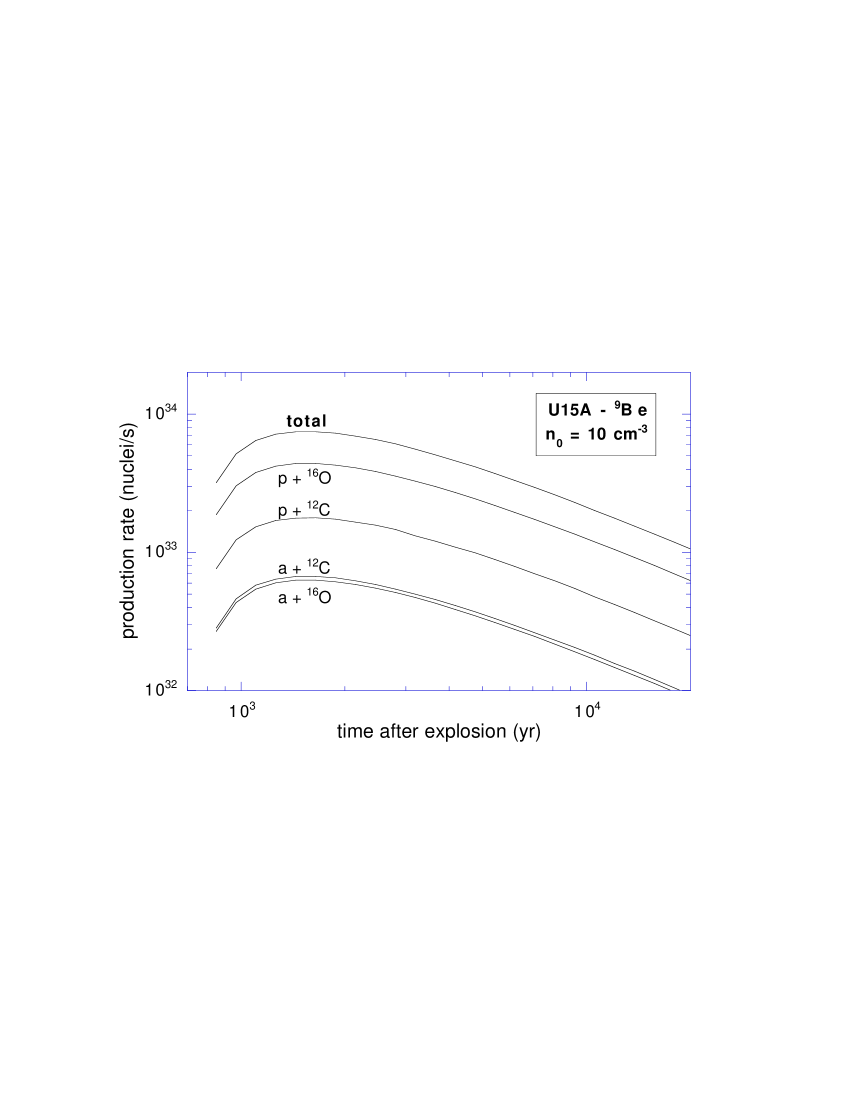
Figure 1: Process 1 ⁹Be production rate in numbers of nuclei per second through different spallation reactions as a function of time after the SN explosion. The SN model used is U15A (from Woosley and Weaver, 1995), and the ambient density is $n_{0}=10\,\mathrm{cm}^{-3}$.

In Fig. 1, we show the typical evolution of the spallation rates for Be production as a function of time, for a SN exploding in a medium with mean density $n_{0}=10\,\mathrm{cm}^{-3}$. The main contribution is seen to come from reaction $\mathrm{p}+^{16}$O, which is due to the low $\mathrm{C}/\mathrm{O}$ abundance ratio in the SN ejecta. For reactions involving alpha particles, this deficiency of carbon as compared to oxygen is compensated by a greater spallation efficiency. The general shape of the curves is easily understood if one refers to Eq. (6) and to the analysis of the preceding section. Indeed, the spallation rates are basically the product of the relevant cross section by the spectral density of energetic protons, $N_{\mathrm{p}}(t)$, and the number density of Oxygen within the SNR. Now the latter is subject to dilution by the swept-up metal-free gas, and therefore decreases as $R^{-3}$, or $R_{\mathrm{SW}}^{-3}(t/\hbox{${t_{\rm SW}}$})^{-6/5}$, while $N_{\mathrm{p}}(t)$ is merely the time integral of the injection function, Eq. (16) (at least as long as one can neglect the energy losses). We thus find $N_{\mathrm{p}}(t)\propto\ln(t/\hbox{${t_{\rm SW}}$})$, and the spallation rates :

$$\frac{\mathrm{d}N_{\mathrm{Be}}}{\mathrm{d}t}\propto R_{\mathrm{SW}}^{-3}(t/\hbox{${t_{\rm SW}}$})^{-6/5}\ln\left(\frac{t}{\hbox{${t_{\rm SW}}$}}\right),$$ (24)

which fits very well the curves in Fig. 1. Differentiating the above expression, we find the maximum production rates to occur at $t=e^{5/6}\hbox{${t_{\rm SW}}$}\approx 2.3\,\hbox{${t_{\rm SW}}$}$, which expresses the best compromise between Oxygen dilution in the SNR and a sufficient injection of EPs since the onset of the acceleration process.

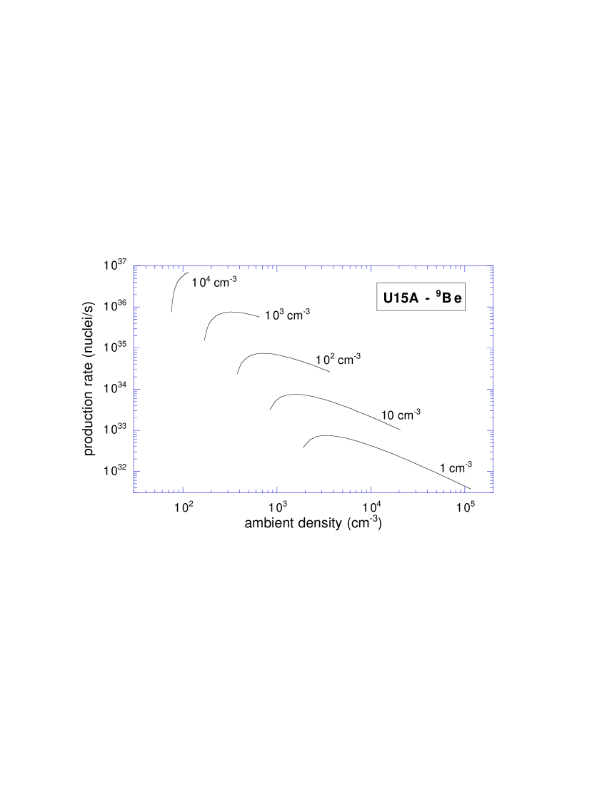
Figure 2: Process 1 total ⁹Be production rates as a function of time after the explosion of SN model U15A, for different ambient densities. Each curve starts shortly after the sweep-up time and ends at the adiabatic time, marking the end of the Sedov-like phase.

This behavior can be further observed on Fig. 2 where we plot the total production rates of Be as a function of time after explosion, for different values of the ambient density, ranging from 1 to $10^{4}\,\mathrm{cm}^{-3}$. The shortening of the Sedov-like phase already mentioned is clearly apparent on the figure, as is the behavior of $\hbox{${t_{\rm SW}}$}\propto n_{0}^{-1/3}$ and $\hbox{${t_{\rm end}}$}\propto n_{0}^{-3/4}$. The calculations also confirm that the position of the maximum is always at $t_{\mathrm{max}}\approx 2.3\,\hbox{${t_{\rm SW}}$}$, although at the highest densities, this is very close indeed to the end of the adiabatic expansion phase, when the confinement of the EPs ceases and the whole process stops. The position of the maximum then varies as $n_{0}^{-1/3}$, while its height, obtained by replacing $t$ by $t_{\mathrm{nax}}$ in Eq. (24), is proportional to $R_{\mathrm{SW}}^{-3}$, and thus $n_{0}$.

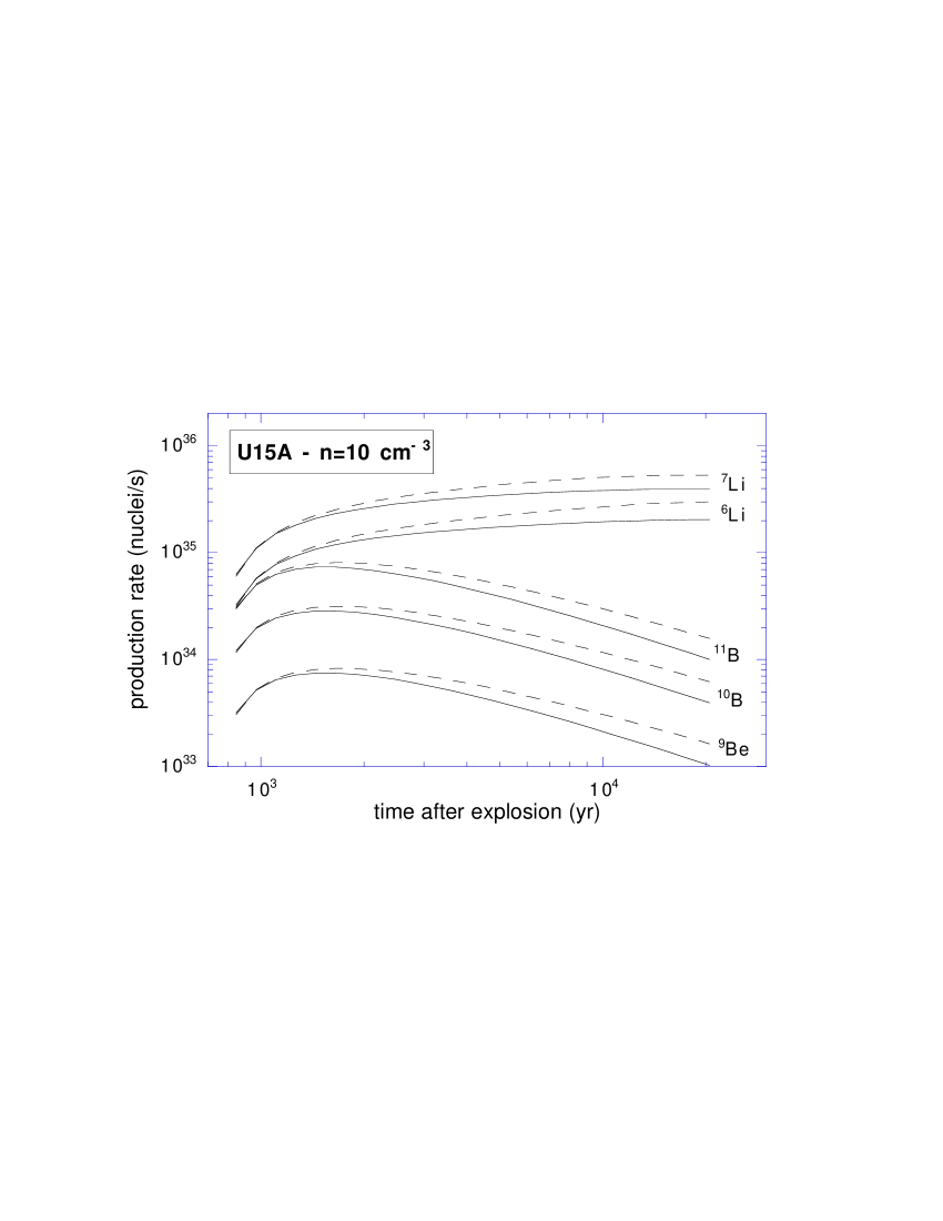
Figure 3: Process 1 production rates of the five light element isotopes as a function of time after the explosion of SN model U15A, in a medium of density $n_{0}=10\,\mathrm{cm}^{-3}$. Results are shown for calculations taking adiabatic losses into account (full lines) as well as ignoring them (dashed lines).

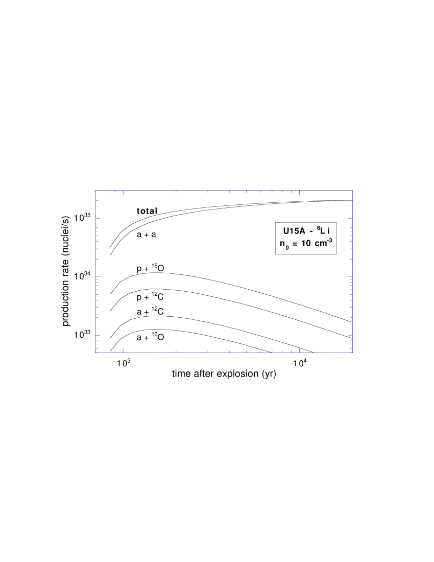
Figure 4: Process 1 ⁶Li production rate in numbers of nuclei per second through different spallation reactions as a function of time after the SN explosion. The SN model used is U15A and the ambient density is $n_{0}=10\,\mathrm{cm}^{-3}$.

In Fig. 3 we show the evolution of the production rates for the five light element isotopes, either taking and not taking the adiabatic losses into account. The behavior of ⁶Li and ⁷Li is different from that of the other isotopes, because lithium is mainly produced through $\alpha+\alpha$ reactions, as shown in Fig. 4, and these reactions are not sensitive to the dilution of the SN ejecta by the ambient material. The evolution of Li production rates therefore reflects directly the evolution of the EP fluxes. As just stated, this would be a pure logarithm if one could neglect the energy losses. It turns out that the adiabatic losses dominate the Coulombian losses for any reasonable ambient density. To see how they influence the EP fluxes, let us re-write Eq. (1) in the form :

$$\frac{\partial}{\partial t}N(E,t)=Q(E,t)-\frac{\partial}{\partial E}(\dot{E}_{\mathrm{ad}}(E,t)N(E,t)),$$ (25)

where we dropped the destruction and second order terms. At energies of a few tens of MeV/n, Eq. (5) simplifies to give the expression for adiabatic losses :

$$\dot{E}_{\mathrm{ad}}(E,t)=-\frac{6}{10}\frac{E}{t}$$ (26)

Replacing in Eq. (25), we obtain :

$$\begin{split}\frac{\partial}{\partial t}N&=Q+\frac{6}{10\,t}\frac{\partial}{\partial E}(EN)\\ &=Q-\frac{6(\alpha-1)}{10\,t}N,\end{split}$$ (27)

where we recognized that a power-law for the injection function $Q$, with spectral index $-\alpha$ ($Q=Q_{0}E^{-\alpha}/t$), translates into a power-law for the EP spectral density $N$ with the same index : $N=N_{0}(t)E^{-\alpha}$. This is a consequence of the proportionality between the energy loss rate and the energy itself. The equation for $N_{0}$ is then straightforward :

$$\frac{\partial}{\partial t}N_{0}=\frac{Q_{0}}{t}-\frac{6(\alpha-1)}{10\,t}N_{0},$$ (28)

from where we see that instead of the logaritmic increase $N(E,t)=Q_{0}E^{-\alpha}\ln(t/\hbox{${t_{\rm SW}}$})$ prevailing in the absence of energy losses, a steady-state value should be reached (if the Sedov-like phase last long enough) with :

$$N_{0}=\frac{10Q_{0}}{6(\alpha-1)}.$$ (29)

So the adiabatic losses are important when both terms in the right hand side of Eq. (28) are of the same order, that is (evaluating the second term from its ‘no-loss value’, and using $\alpha=1.5$ for the low-energy part of the spectrum) :

$$\ln\left(\frac{t}{\hbox{${t_{\rm SW}}$}}\right)\approx\frac{6}{10}(\alpha-1),$$ (30)

or

$$t\la\hbox{${t_{\rm SW}}$}\,e^{\frac{6}{10}(\alpha-1)}\approx 1.35\,\hbox{${t_{\rm SW}}$}.$$ (31)

This result is in very good agreement with the numerical results shown in Fig. 3. Likewise, the gap between the calculations with adiabatic losses turned on or off is increasing only logarithmically with time, so that the difference is rather small, even at the end of the Sedov-like phase. We find total Be production only a few tens of percent higher if we drop the adiabatic losses, and the difference even falls to zero when higher ambient densities are considered. This is of course because the Sedov phase is then considerably shortened.

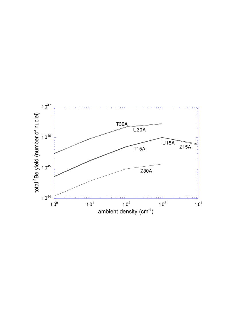
Figure 5: Integrated process 1 Be yields for different SN models as a function of ambient density. For the models with progenitor masses of 30 $M_{\odot}$ and a density higher than a few $10^{3}\,\mathrm{cm}^{-3}$, the sweep-up time ${t_{\rm SW}}$ is greater than the adiabatic time ${t_{\rm end}}$, so that the Sedov-like phase does not exists.

Although Fig. 1, 2 and 3 help us to clarify the dynamics of the process and understand the role of the different parameters, only the total, integrated light elements production is actually relevant to the Galactic chemical evolution. We show in Fig. 5 the results of the integration of the Be production rates over the whole Sedov-like phase, for different SN explosion models, as a function of the ambient density. Except for the case of the Z30A model, we find that for a given mass of the progenitor the total Be yield is independent of the initial metallicity of the star (zero, $10^{-4}$ or $10^{-2}$ times solar). The very small production of Be obtained with the Z30A model is in fact due to a very small amount of Oxygen expelled by the supernova. A model with a higher explosion energy (Z30B) gives results closer to those of T30A and U30A. Although yields significantly different are obtained for different masses of the progenitor, due to different compositions and masses of the ejecta, it is clear from Fig. 5 that the total amount of Be produced by process 1 (forward shock) is much too low to account for the Be observed in metal-poor star. Indeed, the results obtained for a $15\,\hbox{$M_{\odot}$}$ star with ambient density $n_{0}=1\,\mathrm{cm}^{-3}$ are about three orders of magnitude too low, for our choice of $\theta_{1}=0.1$. This is in very good agreement with the analytical estimates presented in Paper I.

Concerning the density dependence of the Be yields, the numerical results shown in Fig. 2 are also in good agreement with the analytical calculations. In particular, the yields increase with ambient density and reach a maximum at about a few $10^{3}\,\mathrm{cm}^{-3}$, above which the Sedov-like phase becomes extremely short, and even vanishes for high mass progenitors (implying large ejected masses). Using Eq. (7) and (8) we can write this limiting density as :

$$n_{\mathrm{lim}}\simeq(4\,10^{4}\,\mathrm{cm}^{-3})\left(\frac{M_{\mathrm{ej}}}{10\,\hbox{$M_{\odot}$}}\right)^{-2}\left(\frac{E_{\mathrm{SN}}}{10^{51}\,\mathrm{erg}}\right)^{3/2}.$$ (32)

4.2 LiBeB production by the EPs from the reverse shock

We now turn to the results obtained for the second mechanism, in which the SN ejecta are accelerated at the reverse shock at the onset of the Sedov-like phase. The ⁶Li and ⁹Be production rates are shown on Fig. 6 as a function of time, with and without adiabatic losses, for an ambient density of $10\,\mathrm{cm}^{-3}$ and a progenitor corresponding to the U15A model of SN. As can be seen, the Be production rates are strongly dominated by inverse spallation reactions, i.e. reactions in which the projectile is the heavier nuclei. Moreover, since the abundance of C and O in the target suffers from dilution by ISM gas, the direct-to-inverse spallation efficiency ratio keeps decreasing during the Sedov-like phase. At the end of it, as already discussed, the direct reactions stop, while inverse ones are not affected. In Figs. 6b and  6d, the adiabatic losses have not been taken into account. The decrease of the direct spallation rates is thus due only to dilution, and we obtain the expected power law in $R^{-3}$, or $t^{-6/5}$. In the meanwhile, the inverse spallation rates are almost constant, as the Sedov-like phase is much shorter than the time-scale for coulombian losses. This time-scale can literally be read from the figure. It is of order a few times $10^{5}$ years for this set of parameters. Note however that the energy loss time-scale actually depends on the species and energy of the particle. Accordingly, what is observed on the spallation rates is in fact a mean coulombian time-scale, averaged over the EP energy spectrum, and more precisely the part of this spectrum which stands above the energy threshold of the cross-sections. This explains the slight variation observed for the different spallation channels.

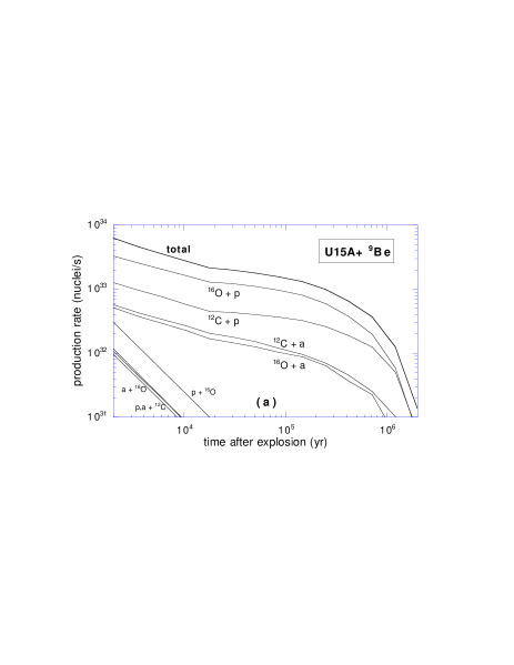
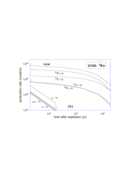
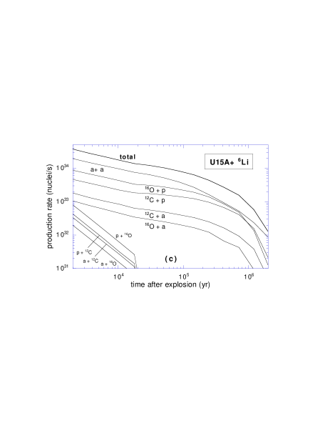
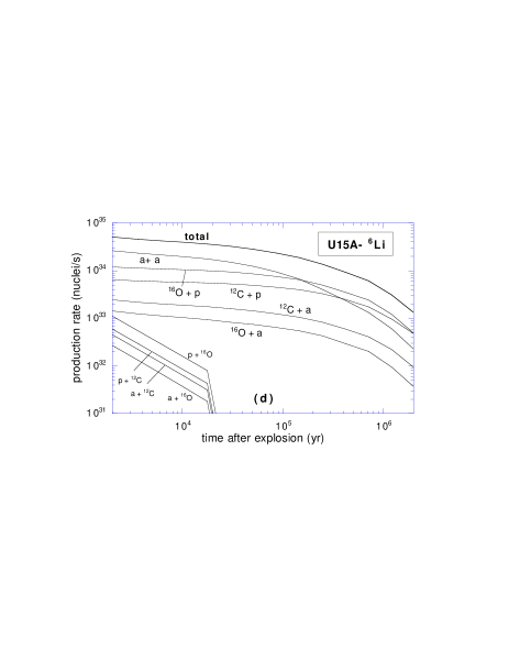
Figure 6: Process 2 (and 3) ⁶Li and ⁹Be production rates in numbers of nuclei per second through different spallation reactions as a function of time after the SN explosion. The SN model used is U15A and the ambient density is $n_{0}=10\,\mathrm{cm}^{-3}$. On the left, the calculations include adiabatic losses (U15A+); on the right, they do not (U15A-).

It is worth emphasizing that the time-scales that we obtain are much shorter than the confinement time-scales inferred from cosmic-ray propagation theories. This indicates that the leakage of the EPs out of the Galaxy has negligible influence on the spallation yields, and justifies our choice of neglecting it. Even for an ambient density of $1\,\mathrm{cm}^{-3}$, the bulk of the light element production is contributed by nuclear reactions occuring within a few million years after the SN explosion, which is to be compared with Galactic confinement times of order a few $10^{7}$ years.

Comparing Fig. 6a with Fig. 6b (or Fig. 6c with Fig. 6d), we can see the influence of the adiabatic losses on the nuclear rates. For inverse spallation reactions, we observe an almost perfect power law decrease, with logarithmic slope $\sim 0.4$, in very good agreement with the value derived in Paper I. Indeed, the analytic treatment led us to expect spallation rates proportional to $R^{-3/4}$, or equivalently $t^{-3/10}$. The slightly quicker decrease found in the numerical results is due to the contribution of the coulombian losses (whose effect is also visible on Figs. 6b and 6d), and to the shape of the spallation cross-sections close to their threshold. Likewise, the time evolution of direct spallation reactions is also very close to a power law, with logarithmic slope of $\sim 1.6\sim(1.2+0.3)$, as expected.

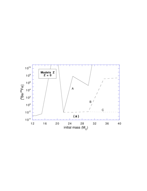
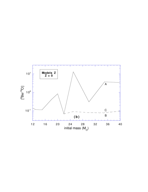
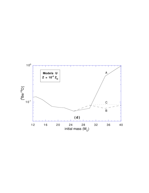
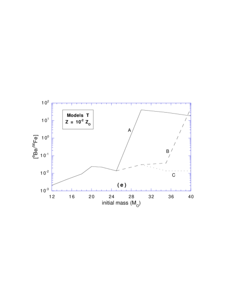
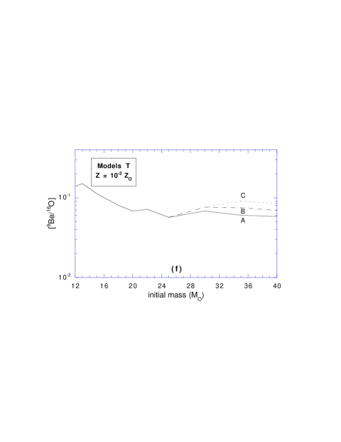
Figure 7: Normalized process 2 [Be/Fe] and [Be/O] yield ratios, as a function of the mass of the progenitor. Models Z, U and T correspond to the indicated initial metallicity of the stars. Models A, B and C correspond to different explosion energies (see text and Woosley and Weaver, 1995). The yield ratios are normalized to the value required by the observations as explained in the text.

As noted above, however instructive the examination of the spallation rates evolution may be, they cannot be directly compared to any observational data. We therefore calculated the (more relevant) integrated yields for different models corresponding to initial metallicities $Z=0$ (models Z), $Z=10^{-4}\,Z_{\odot}$ (models U), and $Z=10^{-2}\,Z_{\odot}$ (models T), and normalized them to the expected value, i.e. to the value required to explain the abundances observed in the metal-poor stars. Consequently, normalized yields respectively lower and higher than 1 are equivalent to under- and over-production of Be. A few words of explaination are however required as how the normalization is actually performed. The only assumption here is that the Galactic Be evolution is primary relative to both Fe and O. This means that the Be/Fe and Be/O ratios are approximately constant in metal-poor stars (as is consequently the O/Fe ratio). Then each supernova must lead, on average (over the IMF), to the same Be/Fe and Be/O ratios as those observed. These are thus the values we use to normalize our results. Now, as the Fe and O yields calculated by Woosley and Weaver (1995) are different for each of their SN models, we applied our normalization model by model and obtained the results shown in Fig.7, as a function of the mass of the SN progenitor, for different initial metallicities.

As discussed earlier, the approximate constancy of the Be/Fe ratio is well established observationally, over two orders of magnitude in metallicity, from $\mathrm{Fe/H}\la 10^{-3}$ to $10^{-1}$ times the solar value. On the other hand, we still lack similar measurements of the Be/O ratio in stars with $\mathrm{O/H}\la 10^{-2}$ times the solar value, while the trend at higher metallicity seems to favour a slightly increasing Be/O, if one is to believe the recent observations by Israelian et al. (1998) and Boesgaard et al. (1998) (see also Fields and Olive, 1999). To this respect, it might seem that our normalization based on the primary behavior of Be is better justified for comparison to Fe than to O. In fact, it is just the opposite. Indeed, the models we are investigating (processes 1 and 2) predict a linear increase of Be as compared to O, whatever the Fe evolution may be. As already noted in Paper I, Be and Fe actually have no direct physical link, as the spallation reactions involve only C and O (and in fact mainly Oxygen, as we have shown; see Figs. 1 and 6). Both processes 1 and 2 could therefore account, in principle, for any value of the Be/Fe ratio, provided we can choose the Iron yield of the SNe (this is however not the case, and even if the SN explosion models entail possibly large uncertainties, the claim for and use of a constant Be/Fe ratio is in fact justified by the observations themselves). On the contrary, the Be/O ratio is entirely determined, at a fundamental level, by the processes we investigate here. A higher mass of Oxygen ejected by the supernova would indeed imply a larger Be yield as well, and conversely.

Except for a few ‘irregular models’ which we shall discuss shortly, Fig. 7 shows that the Be yields obtained by process 2 are significantly smaller than the required values, by about two orders of magnitude when comparison is made with Fe, and roughly one order of magnitude when comparison is made with O. This is again in good quantitative agreement with the results of Paper I, so that we confirm that the processes considered here cannot be responsible for the majority of the Be production in our Galaxy. This conclusion has important implications which have been analysed in Paper I and will be summarized below. Let us now comment the figures in greater detail.

For each series of explosion models (Z, U and T), corresponding to different initial metallicities, Woosley and Weaver (1995) have calculated the yields of a number of elements for progenitors of different masses ranging from 12 to 40 $M_{\odot}$. For the more massive progenitors, they found that the yields of Fe, notably, greatly depended on the mass-cut, which in their models is directly linked to the explosion energy. For example, a 30 $M_{\odot}$ model with a ‘standard’ explosion energy of $1.2\,10^{51}$ erg ejects virtually no Iron at all. Explosion energies greater than the standard value have therefore been explored, leading to higher Fe yields for the most massive stars. We use the same notations as in Woosley and Weaver (1995), i.e. models A, B and C correspond to increasing explosion energies of order 1.2, 2 and $2.5\,10^{51}$ ergs, respectively. In fact, the explosion energy has been adjusted for higher mass progenitors in an ad hoc way in order to obtain approximately the ‘standard’ Fe yield of $\sim 0.1\,\hbox{$M_{\odot}$}$. Therefore, passing from model A to model B, and finally to model C as the progenitor’s mass increases, amounts to ensure that the SN yields of both O and Fe do not vary in dramatic proportions. This is the reason why the curves for models A, B and C connect so smoothly on Figs. 7a-f. In particular, it is worth emphasizing that the results which we obtain for this ‘mixed model’ (A, then B, then C), are remarkably similar whatever the initial metallicity and mass of the progenitor may be. We find in this way $[\mathrm{Be}/\mathrm{Fe}]\sim 0.01$ and $[\mathrm{Be}/\mathrm{O}]\sim 0.1$, where the brackets mean that the yield ratios have been normalized to the required value as described above.

It should be clear, however, that there is no special reason why we should increase the explosion energy for the most massive SN progenitors. In fact, the great sensitivity of the Fe yield to the explosion energy for these stars mostly means, to our opinion, that the SN explosion models are still unable to predict reliable yields (especially at the lowest metallicities; see the huge differences between the models in Fig. 7a). For instance, if we adopt the standard explosion energy (models A), then it is clear from Figs. 7a,c,e that the observed Be/Fe ratio is very easy to reproduce if one assumes that only the most massive stars formed in the early Galaxy. The reason for this success, however, is not that the massive stars (indirectly) produce a lot of Be, but rather that they produce extremely little Fe. In this case, then, a serious Fe underproduction problem will be encountered by the chemical evolution models, so that the high value of the [Be/Fe] should be regarded as somewhat artificial, and rather irrelevant to the question of Be production in the Galaxy. Moreover, such a behaviour is not expected to be found in the curves showing the Be production as compared to the Oxygen. Indeed, as already alluded to, if a particular SN model happens to not eject any substantial amount of O, then it will not lead to any significant Be production either, leaving the [Be/O] ratio virtually unchanged. This can be checked on Figs. 7b,d,f, where all the models are shown to give approximately the same results. The only exceptions arise at low metallicity for models A and can be easily understood. In these cases, indeed, the O yield becomes much lower than the C yield, so that the Be production is actually dominated by spallation reactions involving C. Consequently the Be yield is still quite substantial, while the O yield is very low, which brings about a situation very similar to that encountered with Fe.

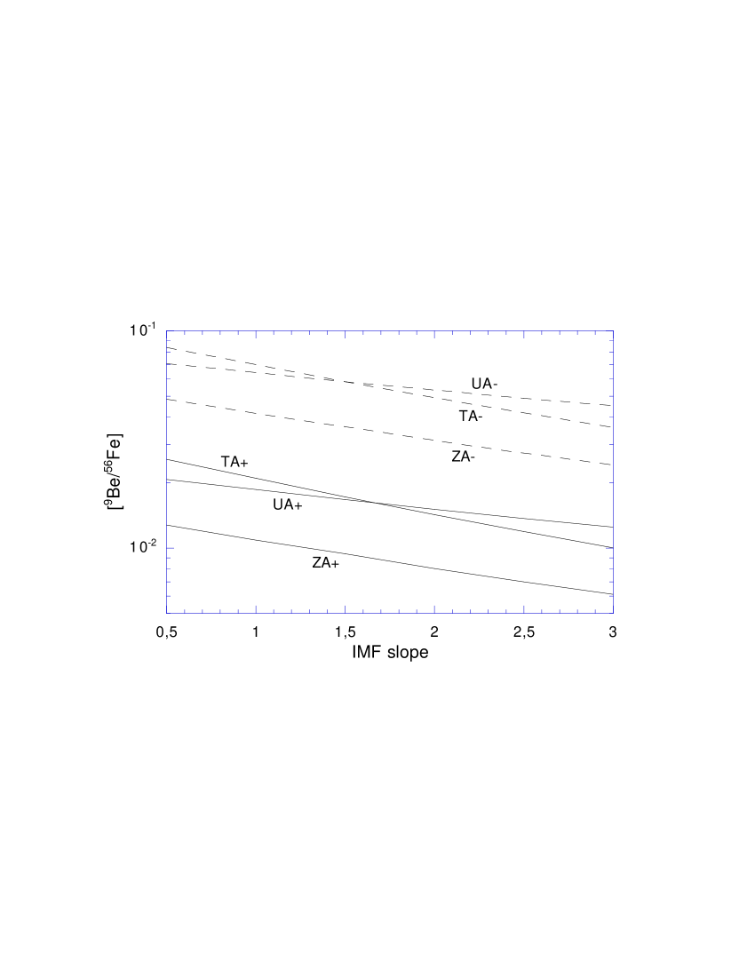
Figure 8: Normalized Be/Fe ratio calculated from SN models ZA, UA, and TA, averaged on the IMF, as a function of the IMF logarithmic slope. (Salpeter slope is 2.35). Models labeled with a ‘+’ include adiabatic losses; those labeled with a ‘-’ (dashed lines) do not.

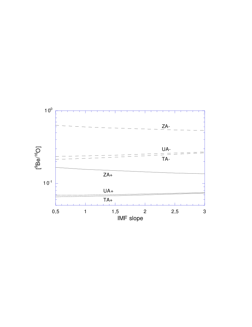
Figure 9: Normalized Be/O ratio calculated from SN models ZA, UA, and TA, averaged on the IMF, as a function of the IMF logarithmic slope. (Salpeter slope is 2.35). Models labeled with a ‘+’ include adiabatic losses; those labeled with a ‘-’ (dashed lines) do not.

However that may be, even if we trust the low (or even extremely low) Fe and O yields obtained from models A for high mass progenitors, the contribution of these high mass SNe still has to be weighted by their frequency among the type II SNe. In Figs. 8 and 9 we show the normalized [Be/Fe] and [Be/O] ratios, after averaging over a power-law IMF with logarithmic slope $x$ ranging from 0.5 to 3. This allows us to explore the influence of varying the weight of the more efficient high mass stars relatively to the lower mass SN progenitors. A low IMF slope (towards 0.5) strongly favours high mass star formation, and is therefore expected to lead to a higher [Be/Fe] ratio than a high IMF slope (towards 3). This qualitative behavior is indeed observed on Figs. 8 and 9, but it can be seen that the effect is actually quite weak, even for such a large range of IMFs. Note that we used ‘IMFs by number’ (of stars), and not ‘IMFs by mass’, so that the Salpeter IMF corresponds to $x=2.35$ in our notations. This means that a slope as low as $x=0.5$ corresponds to an IMF in which more mass is locked in high mass than in low mass stars. Even for such an IMF, the Be/Fe ratio obtained is still less than a few percent of the observed value. Comparing Be to O, it is shown in Fig. 9 that the IMF slope has almost no influence on the normalized [Be/O] ratio, which is a consequence of the strong physical link between the ejected Oxygen and the Be production, as discussed above.

We have also shown, in Figs. 8 and 9, the results obtained without including adiabatic losses (dashed lines). Both [Be/Fe] and [Be/O] ratios are then found to be higher by a factor of about 3 to 4, which is in good quantitative agreement with the analytical calculations of Paper I (see Fig. 5 there). This result has two simple, but important implications. First, it points out the necessity of including the adiabatic losses in the calculations (unless explicitely shown that they do not apply), and therefore of using time-dependent models. Second, it indicates that a model in which the EPs do not suffer adiabatic losses has more chance to succeed in accounting for the observed amount of Be in the halo stars.

5 Conclusion

In conclusion, we have calculated the Be production associated with the explosion of a supernova in the ISM, using a time-dependent model, and confirmed the results of Parizot and Drury (1999) stating that isolated SNe cannot be responsible for the Be observed in the metal-poor stars of the Galactic halo. All the qualitative and quantitative features of the two processes investigated (i.e. acceleration of particles at the forward and the reverse shocks of an isolated supernova) have been found to conform to the analytical expectations. This includes the dependence of the Be yields on the ambient density, the evolution of the spallation rates during and after the Sedov-like phase of the SNR expansion, and the influence of the adiabatic energy losses.

The implications of these results for the Galactic chemical evolution of the light elements have been discussed in detail in Paper I. We shall only stress here that it proves very hard for theoretical models to produce the required amount of Be (and similarly ⁶Li and B) by isolated SNe, according to conventional shock acceleration theory. Indeed, the processes that we investigated tend to optimize the spallation efficiency, in that they either accelerate the freshly synthesized C and O or confine the EPs in an environement much richer in C and O than the surrounding ISM at this stage of chemical evolution. Shock acceleration efficiencies of order 10 percent are also about the maximum that can be expected of any acceleration process. Thinking of a process involving more energy than that released by a SN and/or a higher concentration of C and O than within a SNR is rather challenging.

One promising alternative, however, seems to be a model in which the SNe act collectively, rather than individually, as in the processes investigated in this paper. The idea is that most of the massive stars in the Galaxy are formed in associations (Melnik and Efremov, 1995) and generate superbubbles which expand owing to the cumulated energy released by several consecutive supernovae. This energy leads to strong magnetic turbulence within the superbubble, which is thought to accelerate particles in a very efficient way, according to a specific model developed by Bykov and Fleishman (1992). The interesting feature is that the interior of the superbubble is enriched by significant amounts of C and O previously ejected by stellar winds and SN explosions, so that the accelerated particle should have a primary composition (Parizot et al., 1998; Higdon et al., 1998; Parizot and Knoedlseder, 1998) and therefore be very efficient in producing Be. Moreover, the average energy imparted to the EPs by each supernova is directly related to the explosion energy, instead of only the energy in the reverse shock, as in the process 2 investigated here. Indeed, either that the particles are accelerated directly by the forward shock or that the explosion energy first turns into turbulence and a distrubution of weak secondary shocks (this will be investigated in a forthcoming paper), the total energy imparted to the EPs is expected to be about ten times larger than that assumed for process 2 above (say 10 % of the explosion energy, instead of the $\sim 1\leavevmode\nobreak\ \%$ implied by the use of the reverse shock energy). Further considering that the adiabatic losses would not apply in such a case, we predict an overall factor of about 10 to 30 on the Be yields, depending on the mixing of the ejecta with non enriched ISM within the superbubble. According to the results presented in this paper, this would be enough to account for the [Be/O] ratio observed in the metal-poor halo stars.

Apart from the problem of light element production in the early Galaxy, our calculations have shown that the situation is somewhat different whether we compare Be to Fe or O. This obviously indicates that the Galactic evolution of Fe and O are mutually inconsistent, if one uses the yields of Woosley and Weaver (1995), so that a revision of the SN models should be considered. A similar conclusion has been pointed out by Fields and Olive (1999), who observed that these theoretical yields cannot reproduce the O/Fe slope measured in the abundance diagram. Since the Be problem is found to be less serious when comparison is made with O rather than Fe, we suggest that the Fe rather than the O yields may be responsible for the Fe-O problem. Further observational and theoretical work are however needed to reach a convincing conclusion.

- (1) Boesgaard A. M., King J. R., Deliyannis C. P., Vogt S. S., 1998, in press
- (2) Bykov A. M., Fleishman G. D., 1992, MNRAS, 255, 269
- (3) Duncan D. K., Lambert D. L., Lemke M., 1992, ApJ, 401, 584
- (4) Duncan D. K., Primas F., Rebull L. M., Boesgaard A. M., Deliyannis C. P., Hobbs L. M., King J. R., Ryan S. G., 1997, ApJ, 488, 338
- (5) Edvardsson B., Gustafsson B., Johansson S. G., et al., 1994, A&A, 290, 176
- (6) Fields B. D., Olive K. A., 1999, ApJ, in press
- (7) Gilmore G., Edvardsson B., Nissen P.E., Nissen P. E., 1991, ApJ, 423, 68
- (8) Gilmore G., Gustafsson B., Edvardsson B., Nissen P. E., 1992, Nat, 357, 379
- (9) Higdon J. C., Lingenfelter R. E., Ramaty R., 1998, ApJ, 509, L33
- (10) Israelian G., García-López R. J., Rebolo R., 1998, ApJ, in press
- (11) Kiselman D., Carlsson M., 1996, A&A, 311, 680
- (12) Melnik A. M., Efremov Yu. N., 1995, Astron. Lett., 21, 10
- (13) Molaro P., Bonifacio P., Castelli F., Pasquini L., 1997, A&A, 319, 593
- (14) Parizot E., 1999, A&A, accepted
- (15) Parizot E., Drury L., 1999, A&A, accepted (Paper I)
- (16) Parizot E., Knödlseder J., 1998, in: The transparent Universe, Proceedings of the 3rd INTEGRAL Workshop (Taormina)
- (17) Parizot E., Cassé M., Vangioni-Flam E., 1998, A&A, 328, 107
- (18) Ramaty R., Kozlovsky B., Lingenfelter R. E., Reeves H., 1997, ApJ, 488, 730
- (19) Ryan S., Norris I., Bessel M., Deliyannis C., 1994, ApJ, 388, 184
- (20) Silberbers R., Tsao C. H., 1990, Phys. Rep., 191, 351
- (21) Woosley S. E., Weaver T. A., 1995, ApJSS, 101, 181