GENESIS:
A high–resolution code for 3D relativistic hydrodynamics

Abstract

The main features of a three dimensional, high–resolution special relativistic hydro code based on relativistic Riemann solvers are described. The capabilities and performance of the code are discussed. In particular, we present the results of extensive test calculations which demonstrate that the code can accurately and efficiently handle strong shocks in three spatial dimensions. Results of the performance of the code on single and multi-processor machines are given. Simulations (in double precision) with $\leq 7\,\,10^{6}$ computational cells require less than 1 Gb of RAM memory and $\approx 7\,\,10^{-5}$ CPU seconds per zone and time step (on a SCI Cray–Origin 2000 with a R10000 processor). Currently, a version of the numerical code is under development, which is suited for massively parallel computers with distributed memory architecture (like, e.g., Cray T3E).

1 Introduction

Numerical relativistic hydrodynamics (RHD) has experienced an important step forward in recent years when modern high–resolution shock–capturing (HRSC) techniques began to be applied to solve the equations of RHD in conservation form. Prior to the advent of HRSC techniques the field was dominated for more than one decade by Wilson (1979)’s approach to relativistic hydrodynamics. This approach relies on the use of artificial viscosity in order to handle the discontinuities (shocks, contact discontinuities, etc.) that may appear in the flow numerically. However, techniques based on artificial viscosity are prone to severe numerical difficulties when simulating ultrarelativistic flows (see, e.g., Centrella & Wilson 1984). Using modern HRSC techniques instead, these difficulties are overcome (see, e.g., Donat et al. 1998) allowing one to simulate challenging relativistic astrophysical phenomena like, e.g., relativistic jets or gamma-ray bursts (GRB hereafter).

In astrophysical jets flow velocities as large as $99.5\%$ of the speed of light (Lorentz factors $>10$) are required – according to the nowadays accepted standard model – to explain the apparent superluminal motion observed at parsec scales in many jets of extragalactic radio sources associated to active galactic nuclei. Similar arguments applied to the galactic superluminal sources GRS1915+105 (Mirabel & Rodriguez 1994) and GROJ1655–40 (Tingay et al. 1995) allow one to infer intrinsic velocities of $\approx 0.9c$ in the jets of these sources. Further independent indication of highly relativistic speeds can be inferred from the intraday variability occurring in more than a quarter of all compact extragalactic radio sources (Krichbaum, Quirrenbach & Witzel 1992). If the observed intraday radio variability is intrinsec and results from incoherent synchrotron radiation (according to Begelman, Rees & Sikora 1994), the associated jets must have bulk Lorentz factors in the range $\sim$ 30 – 100.

With exception of the remarkable work of van Putten (1993, 1996), who used pseudo spectral techniques to solve the equations of relativistic magnetohydrodynamics, numerical simulations of relativistic jets started soon after the first multidimensional relativistic HRSC codes had been developed (Martí, Müller & Ibáñez 1994, Duncan & Hughes 1994, Martí et al. 1995). Since then many different aspects of relativistic jets have been investigated (see, e.g., Martí 1997 for a recent review). The morphology, dynamics and propagation properties of relativistic jets have been analysed in Martí et al. (1997). Komissarov & Falle (1997) investigated the long–term evolution of relativistic jets. First simulations of superluminal sources combining relativistic hydrodynamics and synchrotron radiation transfer at parsec scales have been performed by Gómez et al. (1995, 1997) and by Mioduszewski, Hughes & Duncan (1997) and Komissarov & Falle (1997). From their simulations these authors inferred that the observations of such sources can be explained in terms of travelling perturbations in steady relativistic jets.

In the last two years further progress was achieved by simulating relativistic jets in three spatial dimensions and by incorporating magnetic fields (Koide, Nishikawa & Mutel 1996; Nishikawa et al. 1997; Koide 1997). However, instead of using fluxes obtained by solving Riemann problems at zone interfaces, Koide and collaborators code rely on the addition of nonlinear dissipation terms to their Lax–Wendroff scheme to stabilise the code across discontinuities. This stabilisation method was originally proposed by Davis (1984), who applied it successfully to the equations of classical hydrodynamics. The method is robust and simple as no detailed characteristic information is needed. Koide and collaborators did simulate the evolution of the jet only for a very brief period of time. This fact and the coarse grid zoning used in their simulations, however, prevented them from studying genuine 3D effects in relativistic jets in any detail. On the other hand, the relative smallness of the beam flow Lorentz factor (4.56, beam speed $\approx 0.98$) assumed in their simulations does not allow for a comparison with Riemann-solver-based HRSC methods in the ultrarelativistic limit.

An astrophysical phenomenon which also involves flows with velocities very close to the speed of light are gamma-ray bursts (GRB). Although known observationally since over 30 years, their nature and their distance (“local” or “cosmological”) is still a matter of controversial debate (Fishman & Meegan 1995; Mézáros 1995; Piran 1997). In order to explain the energies released in a GRB various catastrophic collapse events have been proposed including neutron-star/neutron-star mergers (Pacyński 1986; Goodman 1986; Eichler et al.1989), neutron-star/black-hole mergers (Mochkovitch et al.1993) collapsars (Woosley 1993) and hypernovae (Pacyński 1998). These models all rely on a common engine, namely a stellar mass black hole which accretes several solar masses of matter from a disk (formed during a merger or by a non-spherical collapse) at a rate of $\sim 1\,\mbox{M}_{\odot}\mbox{s}^{-1}$ (Popham, Woosley & Fryer 1998). A fraction of the gravitational binding energy released by accretion is converted into neutrino and anti-neutrino pairs, which in turn annihilate into electron-positron pairs. This creates a pair fireball, which will also include baryons present in the environment surrounding the black hole. Provided the baryon load of the fireball is not too large, the baryons are accelerated together with the e${}^{+}\,$e^- pairs to ultrarelativistic speeds with Lorentz factors $>10^{2}$ (Cavallo & Rees 1978; Piran, Shemi & Narayan 1993). The bulk kinetic energy of the fireball then is thought to be converted into gamma-rays via cyclotron radiation and/or inverse Compton processes (see, e.g., Mészáros 1995).

In the following we describe the main features of a special relativistic 3D hydrodynamic code, which is based on explicit HRSC methods, and which is a considerably extended version of the special relativistic 2D hydrodynamic code developed by Martí, Müller & Ibáñez (1994) and by Martí et al. (1995). The code has been designed modularly which allows one to use different reconstruction algorithms and Riemann solvers. As it is the final goal of our work to simulate relativistic jets and GRBs in three spatial dimensions, the code has successfully been subjected to an intensive testing in the ultrarelativistic regime (see Section (4)). In particular, GENESIS has successfully passed the spherical shock reflection test (simulated in 3D Cartesian coordinates) involving flow Lorentz factors larger than 700 (see §(4.3)).

The paper is organised as follows. In Section (2), we introduce the 3D equations of RHD in Cartesian coordinates in differential and discretized forms. The latter have been implemented into our 3D RHD code GENESIS. Detailed information about the structure and the main features of the code is given in Section (3). Several 1D, 2D and 3D relativistic test problems computed with GENESIS are described in Section (4). The performance of GENESIS on scalar and multi-processor computers is analysed in Section (5), and a realistic simulation of a 3D relativistic astrophysical jet is presented in Section (6). A summary of the paper containing our main conclusions and a discussion of present and future applications of the code in different astrophysical areas can be found in Section (7). In Appendix A, we give the spectral decomposition of the three dimensional system of RHD equations with explicit expressions for the eigenvalues and the right- and left-eigenvectors. Appendix B contains the explicit formulae for the numerical viscosity for Marquina’s (Donat & Marquina 1996) Riemann solver, and Appendix C describes the explicit algorithm to recover the primitive variables form the conserved ones.

2 Equations of RHD in conservation form

The evolution of a relativistic perfect fluid is described by five conserved quantities: rest mass density, $D$, momentum density, ${\bf S}$, and energy density, $\tau$ (all of them measured in the laboratory frame and in natural units, i.e., the speed of light $c=1$),

$$D = \rho W$$ (1)

$$S^{j} = \rho hW^{2}v^{j}\quad(j=1,2,3)$$ (2)

$$\tau = \rho hW^{2}-p-\rho W,$$ (3)

where the Lorentz factor $W=(1-{\rm v}^{2})^{-1/2}$ and ${\rm v}^{2}=\delta_{ij}v^{i}v^{j}$ (the Einstein summation convention is used here, and $\delta_{ij}$ is the Kronecker symbol). Furthermore, $\rho$ is the rest–mass density, $p$ the pressure and $h$ the specific enthalpy given by $h=1+\varepsilon+p/\rho$ with $\varepsilon$ being the specific internal energy. The components of the vector of variables ${\bf w}\equiv(\rho,v^{i},\varepsilon)^{T}$ are called primitive or physical variables.

The relativistic Euler equations form a system of conservation laws (see, e.g., Font et al. 1994) which can be written in Cartesian coordinates as

$$\frac{\partial D}{\partial t} + \displaystyle{\sum_{j=1}^{3}}\frac{\partial}{\partial x^{j}}(Dv^{j})=0$$ (4)

$$\frac{\partial S^{i}}{\partial t} + \displaystyle{\sum_{j=1}^{3}}\frac{\partial}{\partial x^{j}}(S^{i}v^{j}+{\delta}^{ij}p)=0\>\>\>\>\>\>\>\>\mbox{(i=1, 2, 3)}$$ (5)

$$\frac{\partial\tau}{\partial t} + \displaystyle{\sum_{j=1}^{3}}\frac{\partial}{\partial x^{j}}(S^{j}-Dv^{j})=0$$ (6)

or, equivalently, as

$$\frac{\partial{\bf U}}{\partial t}+\displaystyle{\sum_{j=1}^{3}}\frac{\partial{\bf F}^{j}}{\partial x^{j}}=0\,,$$ (7)

where the vector of unknowns ${\bf U}$ (i.e., the conserved variables) is given by

$${\bf U}=\left(D,\>S^{1},\>S^{2},\>S^{3},\>{\tau}\right)^{T}\,,$$ (8)

and the fluxes are defined by

$${\bf F}^{i} = \left(Dv^{i},S^{1}v^{i}+p\delta^{1i},S^{2}v^{i}+p\delta^{2i},S^{3}v^{i}+p\delta^{3i},S^{i}-Dv^{i}\right)^{T}\,.$$ (9)

The system (7) of partial differential equations is closed with an equation of state $p=p(\rho,\varepsilon)$. Anile (1989) has shown that system (7) is hyperbolic for causal equations of state, i.e., for those where the local sound speed, $c_{s}$, defined by

$$hc_{s}^{2}=\frac{\partial p}{\partial\rho}+(p/\rho^{2})\frac{\partial p}{\partial\epsilon},$$ (10)

satisfies $c_{s}<1$.

The structure of the characteristic fields corresponding to the nonlinear system of conservation laws (7) has explicitly been derived in Donat et al. (1998) and is summarised in Appendix A.

In order to evolve system (7) numerically, one has to discretize the state vector ${\bf U}$ within computational cells. The temporal evolution of the state vector is determined by the flux balance across the zone interfaces of each cell and the contribution of source terms. Using a method of lines (see, e.g., LeVeque 1991), our discretization reads

$$\frac{d{\bf U}_{i,j,k}}{dt} = -\frac{1}{{\Delta}x}\left({\bf\tilde{F}}^{x}_{i+\frac{1}{2},j,k}-{\bf\tilde{F}}^{x}_{i-\frac{1}{2},j,k}\right)-\frac{1}{{\Delta}y}\left({\bf\tilde{F}}^{y}_{i,j+\frac{1}{2},k}-{\bf\tilde{F}}^{y}_{i,j-\frac{1}{2},k}\right)$$ (11)

$$-\frac{1}{{\Delta}z}\left({\bf\tilde{F}}^{z}_{i,j,k+\frac{1}{2}}-{\bf\tilde{F}}^{z}_{i,j,k-\frac{1}{2}}\right)+{\bf S}_{i,j,k}\equiv L({\bf U})\,,$$

where latin subscripts $i$, $j$ and $k$ refer to the $x$, $y$ and $z$ coordinate direction, respectively. ${\bf U}_{ijk}$ and ${\bf S}_{i,j,k}$ are the mean values of the state and source vector (if non zero) in the corresponding three-dimensional cell, while ${\bf\tilde{F}}^{x}_{i\pm\frac{1}{2},j,k}$, ${\bf\tilde{F}}^{y}_{i,j\pm\frac{1}{2},k}$ and ${\bf\tilde{F}}^{z}_{i,j,k\pm\frac{1}{2}}$ are the numerical fluxes at the respective cell interface. Finally, $L({\bf U})$ is a short hand notation of the spatial operator in our method.

At this stage, our system of conservation laws is a system of ordinary differential equations which can be integrated with a large number of algorithms. We have chosen a multistep Runge–Kutta (RK) method developed by Shu & Osher (1988) which can provide second (RK2) and third (RK3) order in time. The explicit form of the algorithms is (subindexes $(i,j,k)$ are ommited to clarify the notation):

1. Prediction step (common for both RK2 and RK3):

   $${\bf U}^{(1)}={\bf U}^{n}+{\Delta}tL({\bf U}^{n})$$ (12)

2. Depending on the order do:

   • RK2:

     $${\bf U}^{n+1}=\frac{1}{\alpha}\left({\beta}{\bf U}^{n}+{\bf U}^{(1)}+{\Delta}tL({\bf U}^{(1)})\right),$$ (13)

     being $\alpha=2$ and $\beta=1$.

   • RK3:

     $${\bf U}^{(2)} = \frac{1}{\alpha}\left({\beta}{\bf U}^{n}+{\bf U}^{(1)}+{\Delta}tL({\bf U}^{(1)})\right)$$

     $${\bf U}^{n+1} = \frac{1}{\beta}\left({\beta}{\bf U}^{n}+2{\bf U}^{(2)}+2{\Delta}tL({\bf U}^{(2)})\right),$$ (14)

     in this case, $\alpha=4$ and $\beta=3$.**

3 The relativistic hydrodynamic code GENESIS

3.1 Code structure

The special relativistic multidimensional hydrodynamic code GENESIS described in detail in the following is a 3D extension of the 2D HRSC hydrodynamic code developed by some of the authors. The 2D code has been successfully used for the simulation of relativistic jets (Martí et al. 1994, 1995, 1997; Gómez et al. 1995, 1997). The main structural features of Martí et al.’s code has been kept, but there are important changes in the computational part. Besides the addition of the third spatial dimension, a large effort has been made to minimise memory requirements and to optimise the performance of the code as well as to enhance its portability.

Like its predecessor, GENESIS evolves the equations of RHD in conservation form using a finite volume approach in Cartesian coordinates. In accordance with the method of lines, we split the discretization process in two parts. First, we only discretize the differential equations in space, i.e. the problem remains continuous in time. This leads to a system of ordinary differential equations (ODEs) in time (11). The numerical fluxes between adjacent cells required for the time integration are obtained by solving the appropriate 1D Riemann problems along the coordinate directions (spatial sweeps). High-order spatial accuracy is achieved by applying a high-order interpolation procedure in space, while high-order accuracy in time is obtained by using high-order ODE solvers.

GENESIS integrates the 3D RHD equations on uniform grids in each spatial direction. In order to have a flexible code GENESIS is programmed to allow for different boundary conditions, spatial reconstruction algorithms, Riemann solvers, ODE solvers for the time integration and external forces. The user selects these options at the preprocessor level, which reduces the number of if–clauses inside the nested 3D loops to a minimum, and thereby maximising the code’s efficiency.

Making the selection at the preprocessing stage has allowed us to obtain a code, which is independent of a specific (shared memory) machine architecture. Hence, it runs on different types of machines and processors. Up to now, we have tested GENESIS on SGI platforms (INDY workstations, Power Challenge and Cray-Origin 2000 arrays), on HP machines (712 workstations and J280 computers), and on a CRAY-JEDI multiprocessor system. As a next step we plan to port GENESIS on a CRAY-T3E massively parallel computer.

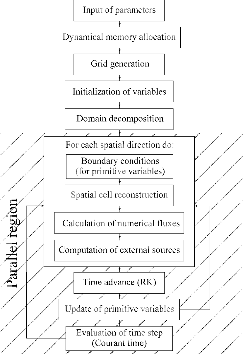
Figure 1: Flow diagram of GENESIS.

The flow diagram of GENESIS is shown in figure 1. Details of the major components of GENESIS are discussed in the following subsections.

3.2 Memory requirements

The current version of GENESIS, which is written in FORTRAN 90 has the capability of allocating memory dynamically, i.e. the number of computational cells can be chosen at run time. Reducing the RAM requirements of a 3D hydrodynamic code is obviously crucial. In GENESIS multidimensional variables are responsible for about $99\%$ of the code’s memory requirement. Thus, the number of these 3D arrays has to be kept at the absolute minimum possible. In its present version, GENESIS only requires three sets of five 3D arrays each, consisting of one set of conserved variables at the begining of each time level (${\bf U}^{n}$), another set of primitive variables and a third set of scratch variables (${\bf\tilde{U}}$). The time integration scheme (eqs. 12–14) which results in the updated values of the conserved variables at the next time level (${\bf U}^{n+1}$) then reads:

1. Prediction step (common for RK2 and RK3):

   $${\bf\tilde{U}}={\bf U}^{n}+{\Delta}tL({\bf U}^{n})$$

2. Depending on the order of accuracy of the time integration scheme do:

   • $${\bf\tilde{U}} = {\bf\tilde{U}}+{\Delta}tL({\bf\tilde{U}}),$$

     $${\bf U}^{n+1} = \frac{1}{\alpha}\left({\beta}{\bf U}^{n}+{\bf\tilde{U}}\right),$$

     with $\alpha=2$ and $\beta=1$, or

   • $${\bf\tilde{U}} = {\bf\tilde{U}}+{\Delta}tL({\bf\tilde{U}}),$$

     $${\bf\tilde{U}} = \frac{1}{\alpha}\left({\beta}{\bf U}^{n}+{\bf\tilde{U}}\right),$$

     $${\bf\tilde{U}} = {\bf\tilde{U}}+{\Delta}tL({\bf\tilde{U}}),$$

     $${\bf U}^{n+1} = \frac{1}{\beta}\left({\beta}{\bf U}^{n}+2{\bf\tilde{U}}\right),$$

     with $\alpha=4$ and $\beta=3$.

Quantities like entropy, internal energy, sound speed or Lorentz factor are implemented as FORTRAN scalars. Consequently, GENESIS needs about 1 Gbyte of RAM memory to handle a grid of $100\times 100\times 720$ (in double precision).

3.3 Domain decomposition

The technique of domain decomposition is used to optimise the parallelization of the code and to guarantee its performance in real applications, too. It is also the first step towards the development of a parallel version of GENESIS which runs efficiently on parallel computers with distributed memory.

The physical domain is split along one arbitrary spatial direction (z, in the present version) in a set of subdomains (i.e. slices, see Fig. 2a) of similar computational load. The subdomains are then distributed across processors. Numerical fluxes at subdomain boundaries are calculated by providing the appropriate internal and external boundary conditions (see Fig. 2b,c, respectively, and § 3.4).

3.4 Boundary conditions

The computational grid is extended in each coordinate in positive and negative direction by four so-called ghost zones, which provide a convenient way to implement different types of boundary conditions. These boundary conditions have to be provided in each spatial sweep for all primitive variables. In GENESIS several types of boundary conditions are available including reflecting, inflow, outflow, time-dependent and analytically prescribed boundary conditions.

Flow conditions at subdomain boundaries must be provided, too, in order to calculate numerical fluxes at subdomain interfaces. Hence, subdomains are also enlarged by four ghost zones in each coordinate direction. Note that these ghost zones do overlap with adjacent subdomains (see Fig. 2). The internal boundary conditions in these overlapping regions are defined by copying the corresponding values of the respective adjacent subdomain. For $NS$ subdomains and $NX\times NY\times NZ$ computational zones the number of overlapping cells is $(4+4)\times(NS-1)\times NX\times NY$, i.e. the fraction of overlapping cells is $8\times(NS-1)/NZ$. Hence, for $NS=16$ and $NZ=1000$ (typical of a jet simulation) the fraction of overlapping cells is about 12%.

3.5 Spatial reconstruction

In order to improve the spatial accuracy of the code, we interpolate the values of the pressure, the proper rest–mass density and the spatial components of the four–velocity ($Wv^{i}$) within computational cells. These reconstructed variables are afterwards used to compute the numerical fluxes. Because of the monotonicity of the reconstruction procedures (see below) used in GENESIS, the occurrence of unphysical (i.e., negative) values in the reconstructed profiles of pressure and density are avoided. In addition, reconstructing the spatial components of the four-velocity with monotonic schemes, also prevents the occurrence of unphysical values of the flow velocity, i.e., the flow velocity always remains smaller than the speed of light even in multidimensional calculations.

GENESIS provides, at the preprocessing level, four different types of reconstruction schemes: piecewise constant, linear using the minmod function of Van Leer (1979), parabolic using the piecewise parabolic method, PPM, of Colella & Woodward (1984; see also Martí & Müller 1996) or hyperbolic using the piecewise hyperbolic method, PHM, of Marquina (1994).

3.6 Source terms

Gravity, local radiative processes, etc., are coupled with hydrodynamics through terms on the right hand side of the RHD equations (i.e., via the source terms, ${\bf S}_{i,j,k}$, in Eq. (11)). GENESIS integrates such terms assuming piecewise constant profiles for the source functions.

3.7 Computation of the numerical fluxes

In this paper we use a variant of Marquina’s flux formula (see Donat & Marquina 1996) which has already been shown to work properly in the simulation of relativistic jets in 2D (Martí et al. 1997).

The approach followed by Donat & Marquina (1996) relies on the extension of the entropy–satisfying scalar numerical flux of Shu & Osher (1989) to hyperbolic systems of conservation laws. Given the spectral decomposition of the RHD equations (see Appendix A), the implementation of Marquina’s scheme is straightforward.

The original Marquina’s algorithm computes the contribution to the numerical viscosity of each characteristic field in a different way depending on whether the corresponding eigenvalue (characteristic speed) does change its sign between the left and right states or whether it does not. However, instead of using the original algorithm, we only consider that part which corresponds to characteristic speeds changing their signs between the left and right states of every numerical interface. The modified algorithm has a larger numerical viscosity, but it is more stable and does not involve any if-clause. Hence, it can easily be vectorized.

In the 2D version used in Martí et al. (1997) the left eigenvectors of the Jacobians are calculated numerically by inverting the matrix of right eigenvectors. In GENESIS we use the analytical expressions for the left eigenvectors, which allow one to simplify the computation of the numerical viscosity terms.

The explicit expressions for the numerical fluxes (${\bf\tilde{F}}^{i}$, $i\in{x,y,z}$ in Eq. 11) as a function of the local (reconstructed) primitive and conserved variables are given in Appendix B. Besides its influence on the efficiency of the code, the use of explicit expressions for the left eigenvectors also leads to analytical cancellations in the computation of the numerical viscosity causing a damping of the growth of round-off errors and an improvement of the overall accuracy of the code. Previous versions of GENESIS, in which numerical fluxes were calculated without the use of analytical expressions, suffered from a growth of round-off errors due to the large number of operations involved and due to the finite precision of floating point arithmetics. This growth of errors manifests itself in a gradual loss of symmetry in initially perfectly symmetric problems. Our experience shows that the analytical manipulation of the expressions of the numerical flux together with their appropriate symmetrization (i.e., using commutating formulas for the components of the velocity parallel to cell interfaces) allows one to achieve a perfect numerical symmetry (see §3.10 and §4.2).

3.8 Time advance and time step computation

Time integration is carried out by two different total variation diminishing RK methods developed in Shu & Osher (1988). The user can choose, at preprocessing level, between the RK2 and RK3 algorithm (see eqs. 12–14). Results of similar quality can be obtained either with the RK3 algorithm or with RK2 using smaller time steps. Nevertheless, for a given time step, the computational cost of RK3 is about a factor 1.5 larger than that of RK2.

As in any explicit hydrodynamic code, time steps are limited for stability reasons by the Courant-Friedrichs-Levy (CFL) condition, which is computed using the characteristic speeds. At the end of each time step the size of the new time step is determined as the minimum of the time steps of all subdomains. This requires a global operation across all subdomains. Experience has shown that acceptable CFL numbers lie in the interval $[0.1,0.8]$. CFL numbers larger than $0.8$ can lead to post shock oscillations.

3.9 Recovering primitive variables

The solution of the Riemann problem requires knowledge of the value of the pressure and its thermodynamic derivatives. Given the functional dependence between conserved and primitive variables (see eq. (2)), the recovering procedure can not be formulated in closed form. Instead a kind of iterative method must be used, which is very time consuming. Hence, usage of the recovering procedure should be reduced to the absolute minimum. Therefore, primitive variables are consistently updated from the mean values of the conserved variables after each Runge-Kutta step and their values are stored in a set of 3D arrays.

Our approach is the same as that of Martí, Ibáñez & Miralles (1991) and that of Martí et al. (1997). Its explicit form can be found in Appendix C (see also Martí & Müller 1996). The iterative recovering procedure is based on a second order accurate Newton-Raphson method to solve an implicit equation for the pressure.

In zones where the flow conditions change smoothly the typical number of iterations ranges from 1 to 3 when a relative accuracy of $10^{-10}$ is requested. There exist zones, however, inside shocks or near strong gradients, where the number of iterations required is larger depending on the strength of the shock or the steepness of the gradient. For example, in the shock reflection test in 3D, the shock zone needs about 4 to 8 iterations.

3.10 Some notes on code structure

We have taken special care in designing a numerical code that accurately preserves any symmetries present in the initial data. This is an important point for a code aimed to study, for example, the stability and long term evolution of initially axisymmetric jets.

There exist two potential sources of numerical asymmetries in our code, both of them are related to the fact that floating point arithmetics is not associative. One cause of asymmetries is due to the computation of numerical fluxes in spatial sweeps, which violates what we call henceforth sweep–level symmetry (SLS). In order to guarantee SLS the expressions by which the numerical fluxes are evaluated have been symmetrized (see §3.7).

A second source of (numerically caused) asymmetry arises specifically in 3D codes using directional splitting. It can only be avoided, if the code has a property which we call sweep–coherence symmetry (SCS). It refers to the symmetry of the integration algorithm with respect to the order in which the 1D-sweeps are performed. This symmetry property of the algorithm becomes crucial if an initially spherically symmetric state is considered. We found that its initial symmetry is lost unless special care is taken in the calculation of the Lorentz factor (in the numerical flux routine), which involves the summation of the squares of the three velocity components. To guarantee a perfect sweep–coherence symmetry of the algorithm the addition of the vector components has to be performed in a cyclic manner, i.e. in the X–sweep the components are summed up in ${x,y,z}$ order, in the Y–sweep in ${y,z,x}$ order, and finally in the Z–sweep in ${z,x,y}$ order. Due to the stochastic nature of round-off errors, a violation of the sweep–coherence symmetry manifests itself only in the last few significant digits of the state variables, if the number of time steps is not too large (less than about 3000; see section §4.3).

Given that round–off errors grow sufficiently slow and that they do not interact with the truncation errors due to the finite difference scheme (which can render the scheme unstable), GENESIS does keep the symmetry of an initial state at an acceptable level. We have also tried to develop a version of GENESIS with a perfect 3D symmetry (limited by the Cartesian discretization). For this purpose, we applied the extended partial precision technique in the computation of expressions in which the associative property should be satisfied. The procedure was successful, but increased the total computational costs by more than 30$\%$. All the results presented in the following have been obtained without making use of such a technique.

4 Code Testing

The capabilities of GENESIS to solve problems in special relativistic hydrodynamics are checked by means of three tests calculations that involve strong shocks and a wide range of flow Lorentz factors. In these test runs an ideal gas equation of state with an adiabatic exponent $\gamma$ has been used. All results presented in this section have been obtained with the PPM reconstruction procedure and the relativistic Riemann solver based on Marquina’s flux formula (see previous section for details).

4.1 Mildly Relativistic Riemann Problem (MRRP)

In the first test we consider the time evolution of an initial discontinuous state of a fluid at rest. The initial state is given by $\rho_{L}=10$, $\epsilon_{L}=2$, $v_{L}=0$, $\gamma_{L}=5/3$, $\rho_{R}=1$, $\epsilon_{R}=10^{-6}$, $v_{R}=0$ and $\gamma_{R}=5/3$, where the subscript $L$ ($R$) denotes the state to the left (right) of the initial discontinuity. This test problem has been considered by several authors in the past (in 1D by Hawley, Smarr & Wilson 1984, Schneider et al. 1993, Martí & Müller 1996, Wen, Panaitescu & Laguna 1997; in 2D by Martí et al. 1997). It involves the formation of an intermediate state bounded by a shock wave propagating to the right and a transonic rarefaction propagating to the left. The fluid in the intermediate state moves at a mildly relativistic speed ($v=0.72c$) to the right. Flow particles accumulate in a dense shell behind the shock wave compressing the fluid by a factor of 5 and heating it up to values of the internal energy much larger than the rest-mass energy. Hence, the fluid is extremely relativistic from a thermodynamical point of view, but only mildly relativistic dynamically.

To change this intrinsically one dimensional test problem into a multidimensional one we have rotated the initial discontinuity (normal to the x-axis) by an angle of $45^{o}$ around the y-axis, and then again by an angle of $45^{o}$ around the z-axis. Gas states $L$ and $R$ are placed within a cube of major diagonal equal to 1 that constitutes the 3D numerical grid.

The analytical solution to this test problem can be found in Martí & Müller (1994). Our analysis is restricted to the flow conditions along the major diagonal of the numerical grid, which is normal to the initial discontinuity. Figure 3 shows the solution along the major diagonal at time $t=0.5$. The shock is captured in two to three zones in accordance with the capabilities of HRSC methods. The transonic rarefaction has a smooth profile across the sonic point located at $x=0.5$, and exhibits sharp corners. The contact discontinuity is spread out over roughly three zones.

The absolute global errors (in $L_{1}$ norm given by ${\epsilon}_{\mbox{\small abs}}=\sum_{i,j,k}\,\left|{\bf w}_{i,j,k}^{n}-{\bf w}({\bf x}_{i,j,k},t_{n})\right|\,\Delta x_{i}\Delta y_{j}\Delta z_{k}$, where ${\bf w}_{i,j,k}^{n}$ and ${\bf w}({\bf x}_{i,j,k},t_{n})$ are the numerical and exact solution, respectively) of pressure, density and velocity are given in Table 1 for different grid resolutions at $t=0.5$. Table 1 implies a convergence rate of slightly less than 1 when comparing the errors obtained on the coarsest ($40^{3}$) and the largest ($150^{3}$) grid. This behaviour is expected for multidimensional problems involving discontinuities (see, e.g. LeVeque 1991).

4.2 Relativistic Planar Shock Reflection (RPSR)

This 1D test problem involves the propagation of a strong shock wave generated when two cold gases, moving at relativistic speeds in opposite directions, collide. The problem has been considered as a test for almost any new relativistic hydrodynamic code (Centrella & Wilson 1984; Hawley, Smarr & Wilson 1984; Martí & Müller 1994; Eulderink & Mellema 1994; Falle & Komissarov 1996).

After the collision of the two gases, two shock waves are created in the plane of symmetry of the physical domain propagating in opposite directions. The inflowing gas is heated in the shocks and comes to a rest. The exact solution of this Riemann problem was obtained by Blandford & McKee (1976).

The initial data are $\rho_{L}=1$, $\epsilon_{L}=2.29\,10^{-5}$, $v_{L}=v_{i}$, $\rho_{R}=1$, $\epsilon_{R}=2.29\,10^{-5}$ and $v_{R}=-v_{i}$, where $v_{i}$ is the inflow velocity of the colliding gas.

Figure 4 shows the numerical solution at $t=2.0$ on the left half of a grid having a total of 401 zones. The results obtained in the right half of the grid are strictly symmetric with respect to the collision point ($x=0$), i.e., the sweep–level symmetry (SLS; see section §3.10) is exactly fulfilled. Near $x=0$, the numerical solution shows small errors (of the same order as the mean error in the post-shock state, $0.3\%$) which are due to the wall heating phenomenon (Noh 1987) characterised by an overshooting of the internal specific energy and an undershooting of the proper rest-mass density.

In Table 2 we give the global absolute errors ($L_{1}$ norm) of the primitive variables for different grids at $t=2.0$ and for an inflow velocity $v_{i}=0.999c$. We find a convergence rate about equal to one (see columns 5-7) for all variables.

We can use this test problem to check the robustness of GENESIS in the ultrarelativistic regime. To simplify notation, we define the quantity $\nu=1-v_{i}$, which tends to zero when $v_{i}$ tends to one. Table 3 contains the relative global errors of the primitive variables at $t=2.0$ for a set of calculations performed on a grid of 401 zones, where we have varied $\nu$ from $10^{-1}$ to $10^{-11}$. The latter value corresponds to a Lorentz factor $W=2.24\times 10^{5}$. The relative error of the primitive variables shows a weak dependence on the inflow velocity. It never exceeds $3.5\%$ and for $\nu\geq 10^{-9}$ it is smaller than $1\%$.

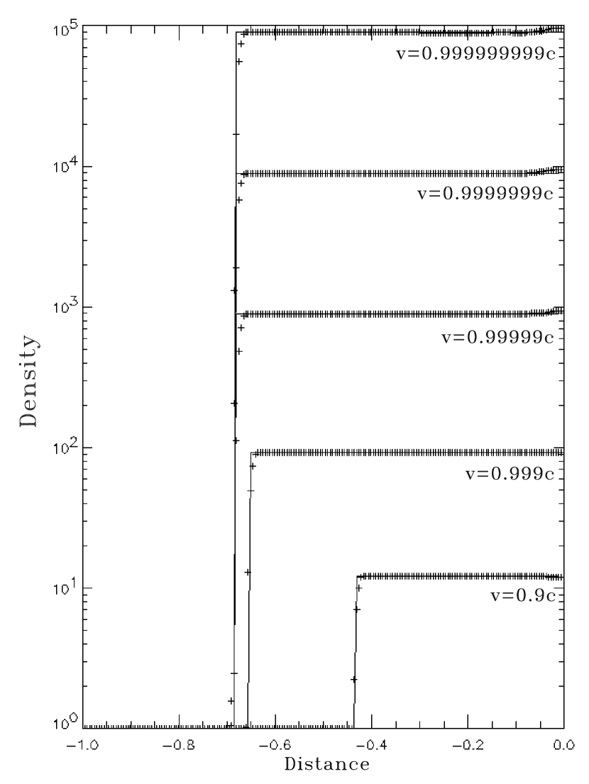
Figure 5: Density jump (in logarithmic scale) for different inflow velocities in the relativistic planar shock reflection problem (RPSR), over an equally spaced grid of $401$ zones at $t=2.0$. As in the previous Figure, only the left half of the grid is shown. Solid lines represent the exact solution while symbols refer to numerical values. A third–order Runge–Kutta was used for time integration.

The PPM parameters (see Colella & Woodward 1984) have been tuned to minimize the number of zones within the shock without introducing unacceptable numerical post–shock oscillations. Fig. 5 demonstrates that there are no numerical post-shock oscillations for $\nu\leq 10^{-5}$ when the shock is captured by 2 to 3 zones.

4.3 Relativistic Spherical Shock Reflection (RSSR)

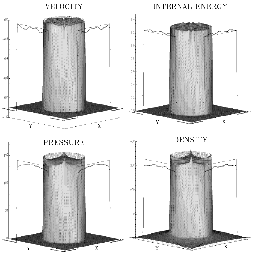
Figure 6: Intensity plots of proper rest–mass density, pressure, specific internal energy and flow velocity over the plane $XY$ at $z=0$ in the relativistic spherical shock reflection test problem (RSSR) described in the text, after 2.0 time units. Shaded surfaces represent the numerical results while dotted surfaces are the exact solution. One dimensional plots along X and Y axes are projected on the front sides of the pictures. Symbols inside the one dimensional plots are numerical values; solid lines represent the exact solution on the same axis. The test was ran using a CFL equal to 0.2 and a third–order Runge–Kutta for time integration.

The initial setup consists of a spherical inflow at speed $v_{i}$ (which might be ultrarelativistic) colliding at the centre of symmetry of a sphere of radius unity. For a hydrodynamic code in Cartesian coordinates this is a 3D test problem, which allows one to evaluate the directional splitting technique as well as the symmetry properties of the algorithm. Figure 6 shows the numerical results for $v_{i}=0.9c$ on a grid of $101^{3}$ zones at $t=2.0$. The shock capturing properties of GENESIS, which we have already demonstrated in 1D, are retained in this genuine multidimensional case. Two or three zones are required to handle the shock wave. The pressure and proper rest–mass density have global relative errors of about $12\%$ and $8\%$ respectively.

Ultrarelativistic flows have been explored by increasing the inflow Lorentz factor. Table 5 gives the growth of the relative global errors (${\epsilon}_{\mbox{\small rel}}={\epsilon}_{\mbox{\small abs}}/\left(\sum_{i,j,k}\,\left|{\bf w}({\bf x}_{i,j,k},t_{n})\right|\,\Delta x_{j}\Delta y_{j}\Delta z_{k}\right)$) on a fixed grid size of $81^{3}$ zones for $v_{i}$ in the range $0.9c$ to $0.999999c$ (the latter inflow velocity corresponding to a Lorentz factor $W\approx 707$). The relative global errors are acceptable (considering the inherent difficulty of the test and the resolution of the experiments) and do not grow dramatically with the Lorentz factor. The observed growth can be explained by the fact that the errors are dominated by the shock region and that the shock strength increases with the Lorentz factor.

The CFL factors used in the last two tests of this series are unusually small ($0.019$ and $0.005$) which is due to the strength of the shock and the relatively small grid resolution (compared with the 1D case). It is noticeable that for $v_{i}=0.999999c$ the errors are considerably larger (last entry in Table 5). This has two reasons. Firstly, the global relative errors decrease with time in the RSSR test problem. Secondly, we could not continue the run with $v_{i}=0.999999c$ beyond 1.5 time units, because interaction with the grid boundaries became severe causing the code to crash. Hence, $v_{i}=0.999999c$ must be considered as the maximum inflow velocity in the RSSR test problem, which the present code can handle properly (for the resolution used). The symmetry properties of the RSSR solution are very well maintained by GENESIS, even though the number of timesteps was very large ($>30000$) in the last two test runs.

The absolute global errors ($L_{1}$ norm) and the convergence rates of the primitive variables at $t=2.0$ are displayed in Table 4. Obviously, the errors are much larger in the 3D test than in the corresponding 1D one. This can be explained considering that (i) the grids are coarser than in 1D, and that (ii) the jumps in pressure and density across the shock are nearly a factor of 30 larger in the 3D test than in the planar case.

The preservation of the sweep-level symmetry (SLS; see section §3.10) is reflected in the symmetry of the one dimensional profiles in Fig. 6. Moreover, a comparison of the profiles in X and Y direction in Fig. 6 shows the capability of the code to maintain the sweep-coherence symmetry (SCS), too.

5 Code Performance

We have parallelized GENESIS in order to run on multiprocessor computers with shared memory. Appart from the initial setup of variables, the grid generation and the output, the rest of the program is organised in a 4-level nested loop. The outermost loop runs from one to the total number of sub-domains, assigning one sub-domain to each processor. This procedure allows an almost complete parallelization of the code employing the corresponding parallelization directives (see Fig. 1).

The MRRP and RSSR tests have been run for different grids on a SGI Cray-Origin 2000 computer. Tables 6 and 7 show the total execution time for every run as a function of the number of CPUs used. We also give the speed up factor, defined as the CPU ratio between a one processor run and one using several processors in parallel. This factor is a measure of the degree of parallelization of the code and should ideally be equal to the number of CPUs used. The tables also contain the execution time per cell and time iteration (TCI). The TCI for a given number of processors is nearly independent of the number of computational cells, and can be used as a time unit to estimate the total execution time needed in a particular simulation.

According to the data shown in Tables 6 and 7 the TCI is about $7.6\,\,10^{-5}$, $2.1\,\,10^{-5}$ and $1.3\,\,10^{-5}$ seconds for 1, 4 and 8 processors, respectively. A significant drop of the performance is noticeable for a grid of $64^{3}$ zones due to the phenomenon of cache trashing, because in this case the dimensions of the 3D matrices are multiples of the size of cache lines. Hence, different 3D matrices are mapped into the same set of cache lines, and every time the program needs to reference a new 3D matrix all cache lines are updated.

Concerning the speed up factor, it is noticeable from Tables 6 and 7 that it increases with the number of grid points, because the 3D nested loops consume a larger percentage of the total CPU time when the number of grid zones is larger. The maximum speed up factors are 3.7 and 6.5 for 4 and 8 CPUs, respectively. We also notice a super linear behaviour, for the largest grid, for the MRRP test problem. As typical 3D simulations are performed with zone numbers larger than the ones used in the test runs, we expect to reach even larger speed up factors in these applications.

The number of Mflops (millions of floating point operations per second) achieved by the code is about 60 on one processor (R10000) of a SGI Cray–Origin 2000 computer. The theoretical peak speed of such a processor is 400 Mflops. For comparison, Pen (1998) reports a performance of 48 Mflops for his 3D adaptive moving mesh classical hydrodynamic code using a SGI Power Challenge machine with R8000 processors (300 Mflops theoretical peak speed).

Finally, we compare the performance of GENESIS achieved on the PA8000 processor of Hewlett Packard with that obtained on the R10000 processor of Silicon Graphics. For the comparison we used a HP J280 workstation equipped with a PA8000 processor with a 180 MHz clock and a cache memory of 512 Kbytes and a SGI Cray-Origin 2000 equipped with a R10000 processor with a 195 MHz clock and 4 Mbytes of cache memory. The test problem selected for the comparison was the relativistic spherical shock reflection test (RSSR) with an inflow velocity of $0.9c$. Test runs were done with four different grids. The resulting execution times per zone and time step (TCI) are given in Table 8.

We find that $\mbox{TCI}_{HP}\approx 2\times\mbox{TCI}_{SGI}$. From Table 8 we can infer a general trend. The TCIs obtained on both machines tend to become similar when the number of zones increases. Furthermore, the TCI for the HP machine is nearly independent of the number of zones, while the TCI for the SGI machine increases with that number. This behaviour may result from the fact that the problem size always leads to an overflow of the cache memory on the HP workstation, while this does not generally happen for the larger cache memory of the SGI machine.

6 An astrophysical application: axisymmetric jet in 3D

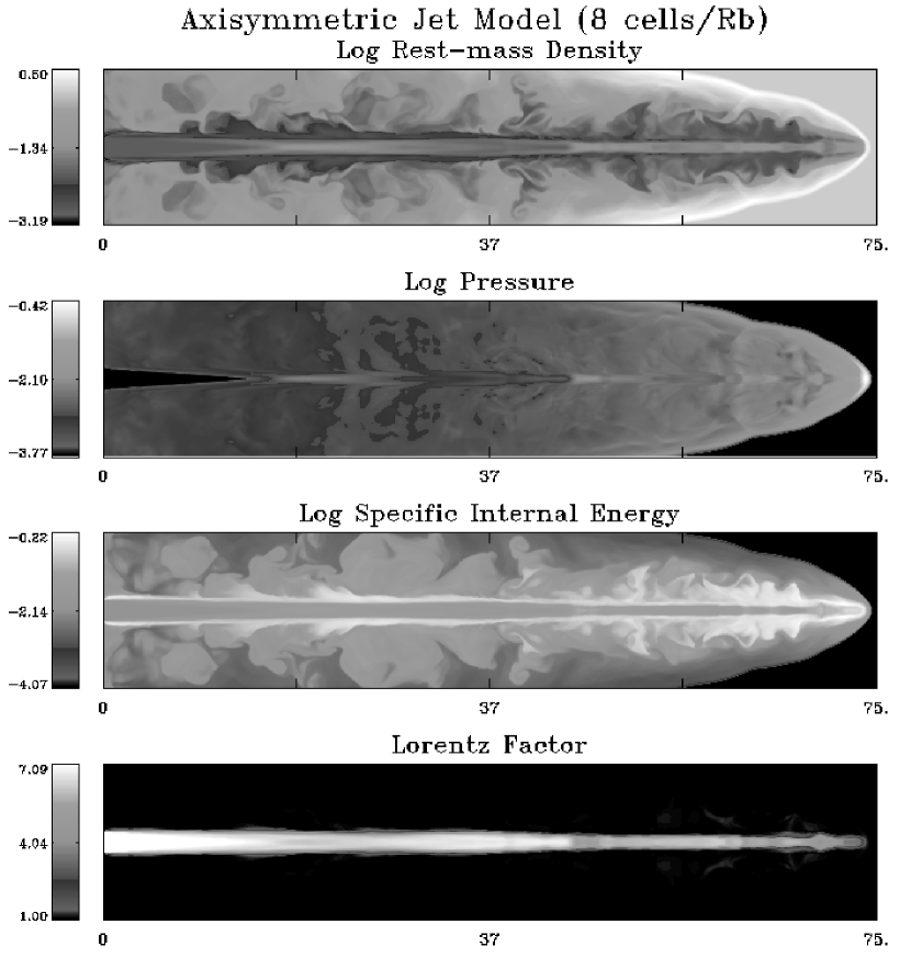
Figure 8: Same as Fig. 7 but with a resolution of 8 zones$/R_{b}$.

Next we discuss an astrophysical application computed with GENESIS, namely the 3D simulation of a relativistic jet propagating through an homogeneous atmosphere. The properties of the jet are those of model C2 in Martí et al. (1997). The beam flow velocity, $v_{b}=0.99c$, the beam Mach number, ${\cal M}_{b}=6.0$, and the ratio of the rest-mass density of the beam and the ambient medium ${\eta}=0.01$. The ambient medium is assumed to fill a Cartesian domain (X,Y,Z) with a size of $15R_{b}\times 15R_{b}\times 75R_{b}$, where $R_{b}$ is the beam radius. The jet is injected at $z=0$ in the direction of the positive $z$-axis through a circular nozzle defined by $x^{2}+y^{2}\leq R_{b}^{2}$, and is in pressure equilibrium with the ambient medium. An ideal gas equation of state with an adiabatic exponent $\gamma=5/3$ is assumed to describe both the jet matter and the ambient gas. Two different spatial resolutions with 4 and 8 zones per beam radius were used in our calculations (Figs. 7,8).

In Martí et al. (1997) the simulation was performed in cylindrical coordinates assuming axial symmetry. The spatial resolution was 20 zones per beam radius both in the axial and radial directions. It is well known that the propagation of a supersonic jet is governed by the interaction of jet matter with the ambient medium, which produces a bow shock in the ambient medium and an envelope surrounding the central beam (the cocoon, in the Blandford & Rees 1974 model). The cocoon contains jet material deflected backward at the head of the jet. In the case of highly supersonic jets, discussed in Martí et al. (1997), extensive, overpressured cocoons are formed with large vortices of jet matter propagating down the cocoon/ambient medium interface. The vortices are the result of Kelvin–Helmholtz instabilities at the interface between the jet and the shocked ambient medium. The interaction of these vortices with the central beam causes internal shocks inside the beam. These, in turn, affect the advance speed of the jet making it highly non–stationary. The propagation speed of the jet can be estimated from the momentum transfer between the jet and the ambient medium assuming a one dimensional flow. For model C2 one obtains an advance speed equal to $0.42c$, whereas the 2D hydrodynamic simulation presented in Martí et al. (1997) gives a mean jet advance speed of $0.37c$.

The four panels in Figs. 7,8 display, from top to bottom, the logarithm of the proper rest-mass density, pressure and specific internal energy and flow Lorentz factor in the plane $x=0$ at $t=160R_{b}/c$, when the jet has propagated about 75 $R_{b}$. The analysis of cross sections of the grid perpendicular to the the jet’s direction of propagation (not shown here) reveals acceptable symmetry of the numerical simulation, i.e both the SLS and the SCS properties are maintained (see §3.10).

The gross morphological and dynamical properties of highly supersonic relativistic jets as inferred from our 3D simulations are qualitatively similar to those established in earlier 2D simulations. An extensive, overpressured cocoon with pressure about 20 times that in the beam at the injection point is found surrounding the jet. The pressure and density at the head of the jet in the model with 8 zones$/R_{b}$ are a factor of 2 larger and 1.3 smaller, respectively, than in the 2D calculation. For the model with 4 zones$/R_{b}$ these factors are 1 and 1.3, respectively. In contrast with the model with 4 zones$/R_{b}$, in which the propagation speed coincides with the 1D estimate, the larger pressure at the head of the jet in the model with 8 zones$/R_{b}$ causes it to propagate through the ambient medium at a larger speed in the 3D calculation ($0.47c$ instead of $0.42c$ for the 1D estimate and $0.37c$ for the 2D simulation) producing a narrower profile of the bow shock near the head. In all the simulations, the supersonic beam displays rich internal structure with oblique shocks effectively decelerating the flow in the beam from a Lorentz factor equal to 7 at the injection point down to a value of about 4 near the head. Whereas gross morphological properties are qualitatively similar in all three simulations, finer jet details (e.g., number, size, position and development of turbulent vortices in the cocoon) do not agree. However, it has been pointed out before that the fine structure is highly dependent on the numerical grid resolution (see, e.g., Kössl & Müller 1988). In the model with 4 zones/$R_{b}$ (see Fig. 7), the material deflected at the head of the jet forms a thick, stable overpressured cocoon surrounding the beam up to the nozzle. Due to the small resolution only large vortices develope in the cocoon/external medium surface which grow slowly. A turbulent cocoon with smaller vortices growing at a faster rate (much more similar to the one obtained in the 2D cylindrical model) are obtained by doubling the resolution (compare, e.g., the proper rest–mass density pannels in Figs. 7,8).

7 Conclusions and Future Developments

We have described the main features of a novel three dimensional, high–resolution special relativistic hydrodynamic code GENESIS based on relativistic Riemann solvers. We have discussed several test problems involving strong shocks in three dimensions which GENESIS has passed successfully. The performance of GENESIS on single and multiprocessor machines (HP J280 and SGI Cray–Origin 2000) has been investigated. Typical simulations (in double precission) with up to $7\,10^{6}$ computational cells can be performed with 1Gbyte of RAM memory with a performance of $\approx 7\,10^{-5}$ s of CPU time per zone and time step (on a SCI Cray-Origin 2000 with a R10000 processor). Currently we are working on a version of GENESIS suited for massively parallel computers with distributed memory (like, e.g., Cray T3E).

GENESIS has been designed to handle highly relativistic flows. Hence, it is well suited for three dimensional simulations of relativistic jets. First results will be presented in a separate paper (Aloy et al. 1998). Further applications envisaged are the simulation of relativistic outflows from merging compact objects (see, e.g., Ruffert et.al. 1997), from hypernovae (Paczynski 1998), or collapsars (MacFadyen & Woosley 1998). In all these models ultra-relativistic outflow is thought to occur and to play a crucial role in the generation of gamma-ray bursts.

ACKNOWLEDGEMENTS

This work has been supported in part by the Spanish DGICYT (grant PB94-0973 and Acción Integrada hispano-alemana HA1996-0154). MAA expresses his gratitude to the Conselleria d’Educació i Ciència de la Generalitat Valenciana for a fellowship. The authors gratefully acknowledge the collaboration of the User’s Support Service of the Centre Europeu de Paral$\cdot$lelisme de Barcelona (CEPBA). The calculations were carried out on a HP J280 and on two SGI Origin 2000, at CEPBA and at the Centre de Informática de la Universitat de València.

Appendix A Characteristic fields of the RHD equations

Analytical expressions for the spectral decomposition of the three $5\times 5$ (in 3D) Jacobian matrices ${\bf\cal B}^{i}({\bf U})$ associated to the fluxes ${\bf F}^{i}({\bf U})$ of system (7),

$${\bf\cal B}^{i}({\bf U})=\frac{\partial{\bf F}^{i}({\bf U})}{\partial\bf U\rm}$$ (A1)

have been given by Donat et al. (1998).

In this Appendix, we explicitly show the eigenvalues and the right and left eigenvectors coresponding to matrix ${\bf\cal B}^{x}$, whereas the cases $y$ and $z$ easily follows from symmetry. The eigenvalues are:

$$\lambda_{\pm}=\frac{1}{1-{\rm v}^{2}c_{s}^{2}}\left\{v^{x}(1-c_{s}^{2}){\pm}c_{s}\sqrt{(1-{\rm v}^{2})[1-v^{x}v^{x}-({\rm v}^{2}-v^{x}v^{x})c_{s}^{2}]}\right\}$$ (A2)

$$\lambda_{0}=v^{x}\mbox{\,\,\,\,(triple)}$$ (A3)

The following expressions define auxiliary quantities:

$${\cal K}\equiv{\displaystyle{\frac{\tilde{\kappa}}{\tilde{\kappa}-c_{s}^{2}}},\>\>\>\>{\tilde{\kappa}}=\frac{1}{\rho}\left.\frac{\partial p}{\partial\varepsilon}\right|_{\rho}},\>\>\>\>{\cal A}_{\pm}\equiv{\displaystyle{\frac{1-v^{x}v^{x}}{1-v^{x}{\lambda}_{\pm}}}}$$ (A4)

A complete set of right–eigenvectors is,

$${\bf r}_{0,1}=\left({\displaystyle{\frac{{\cal K}}{hW}}},v^{x},v^{y},v^{z},1-{\displaystyle{\frac{{\cal K}}{hW}}}\right)$$ (A5)

$${\bf r}_{0,2}=\left(Wv^{y},2hW^{2}v^{x}v^{y},h(1+2W^{2}v^{y}v^{y}),2hW^{2}v^{y}v^{z},2hW^{2}v^{y}-Wv^{y}\right)$$ (A6)

$${\bf r}_{0,3}=\left(Wv^{z},2hW^{2}v^{x}v^{z},2hW^{2}v^{y}v^{z},h(1+2W^{2}v^{z}v^{z}),2hW^{2}v^{z}-Wv^{z}\right)$$ (A7)

$${\bf r}_{\pm}=(1,hW{\cal A}_{\pm}{\lambda}_{\pm},hWv^{y},hWv^{z},hW{\cal A}_{\pm}-1)$$ (A8)

The corresponding complete set of left–eigenvectors is

$${\bf l}_{0,1}={\displaystyle{\frac{W}{{\cal K}-1}}}(h-W,Wv^{x},Wv^{y},Wv^{z},-W)$$

$${\bf l}_{0,2}={\displaystyle{\frac{1}{h(1-v^{x}v^{x})}}}(-v^{y},v^{x}v^{y},1-v^{x}v^{x},0,-v^{y})$$

$${\bf l}_{0,3}={\displaystyle{\frac{1}{h(1-v^{x}v^{x})}}}(-v^{z},v^{x}v^{z},0,1-v^{x}v^{x},-v^{z})$$

$${\bf l}_{\mp}=({\pm}1){\displaystyle{\frac{h^{2}}{\Delta}}}\left[\begin{array}[]{c}hW{\cal A}_{\pm}(v^{x}-{\lambda}_{\pm})-v^{x}-W^{2}({\rm v}^{2}-v^{x}v^{x})(2{\cal K}-1)(v^{x}-{\cal A}_{\pm}{\lambda}_{\pm})+{\cal K}{\cal A}_{\pm}{\lambda}_{\pm}\\ \\ 1+W^{2}({\rm v}^{2}-v^{x}v^{x})(2{\cal K}-1)(1-{\cal A}_{\pm})-{\cal K}{\cal A}_{\pm}\\ \\ W^{2}v^{y}(2{\cal K}-1){\cal A}_{\pm}(v^{x}-{\lambda}_{\pm})\\ \\ W^{2}v^{z}(2{\cal K}-1){\cal A}_{\pm}(v^{x}-{\lambda}_{\pm})\\ \\ -v^{x}-W^{2}({\rm v}^{2}-v^{x}v^{x})(2{\cal K}-1)(v^{x}-{\cal A}_{\pm}{\lambda}_{\pm})+{\cal K}{\cal A}_{\pm}{\lambda}_{\pm}\end{array}\right]$$

where $\Delta$ is the determinant of the matrix of right-eigenvectors.

$$\Delta=h^{3}W({\cal K}-1)(1-v^{x}v^{x})({\cal A}_{+}{\lambda}_{+}-{\cal A}_{-}{\lambda}_{-})$$ (A9)

For an ideal gas equation of state it can be proven that ${\cal K}$ is always greater than one (in fact ${\cal K}$ = $h$), and $\Delta$ is different from zero ($\mid v^{x}\mid<1$).

Appendix B Numerical fluxes and disipation terms in Marquina’s flux formula

Given a cell interface, the numerical fluxes accross such interface are given, in our modified version of Marquina’s flux formula, by

$${\bf\tilde{F}}=\frac{1}{2}\left({\bf F}^{L}+{\bf F}^{R}+{\bf Q}\right).$$ (B1)

In the above expression, ${\bf F}^{L}$ and ${\bf F}^{R}$ are the fluxes at the left and right side of the interface and ${\bf Q}$ is a five–vector containing the numerical viscosity terms which is calculated according to ${\bf Q}={\bf Q}^{R}-{\bf Q}^{L}$.

Quantities ${\bf Q}^{S}$ ($S=L,R$) are written as a sum involving the projectors onto each eigenspace (i.e., direct products of left and right eigenvectors) and the eigenvalues of the corresponding Jacobian matrix

$$Q^{S}_{j}=\sum_{i,k=1}^{5}|\lambda_{i}|_{\mbox{max(L,R)}}\,\,r^{S}_{ji}\,\,l^{S}_{ik}\,\,U^{S}_{k},\,\,\,\,\,\,\,(j=1,\ldots,5).$$ (B2)

Quantities $|\lambda_{i}|_{\mbox{max(L,R)}}$ ($i=1,\ldots,5$) are the maximum of the modulus of the two corresponding eigenvalues at the left and right side of the interface, whereas $r^{S}_{ij}$ ($l^{S}_{ij}$) with $i,j=1,\ldots,5$, refer to the $i$ ($j$) component of the right (left) eigenvector $j$ ($i$). In this expression, subscripts ${1,\ldots,5}$ correspond to ${-,0,0,0,+}$ as defined in Appendix A. $U^{S}_{k}$ are the components of the vector of unknowns. The superscript $S$ indicates that the various qunatities are calculated at each side of the interface in terms of the reconstructed variables.

Omitting the superscript $S$ (the expressions are identical for the left and right side of the interface) one derives the following analytical formulas for $Q_{j}^{S}$:

$$Q_{1} = \frac{h}{\Delta}\left\{M\left[{\cal A}_{-}{\Omega}_{+}-{\cal A}_{+}{\Omega}_{-}\right]+p(\tilde{\lambda}_{+}\tilde{l}_{+}-\tilde{\lambda}_{-}\tilde{l}_{-})\right\}+$$

$$\tilde{\lambda}_{0}p\frac{W}{h}\left\{\frac{{\cal K}}{{\cal K}-1}+\frac{v_{t}^{2}+v_{tt}^{2}}{1-v_{n}^{2}}\right\}$$

$$Q_{2} = \frac{h^{2}W}{\Delta}\left\{M{\cal A}_{+}{\cal A}_{-}\left[{\Omega}_{+}\lambda_{+}-{\Omega}_{-}\lambda_{-}\right]+p(\tilde{\lambda}_{+}\lambda_{+}{\cal A}_{+}\tilde{l}_{+}-\tilde{\lambda}_{-}\lambda_{-}{\cal A}_{-}\tilde{l}_{-})\right\}+$$

$$\tilde{\lambda}_{0}pW^{2}v_{n}\left\{\frac{1}{{\cal K}-1}+2\frac{v_{t}^{2}+v_{tt}^{2}}{1-v_{n}^{2}}\right\}$$

$$Q_{3} = \frac{h^{2}W}{\Delta}v_{t}\left\{M\left[{\Omega}_{+}{\cal A}_{-}-{\Omega}_{-}{\cal A}_{+}\right]+p(\tilde{\lambda}_{+}\tilde{l}_{+}-\tilde{\lambda}_{-}\tilde{l}_{-})\right\}+$$

$$\tilde{\lambda}_{0}p\left\{\frac{W^{2}}{{\cal K}-1}+\frac{1+2W^{2}(v_{t}^{2}+v_{tt}^{2})}{1-v_{n}^{2}}\right\}$$

$$Q_{4} = \frac{h^{2}W}{\Delta}v_{tt}\left\{M\left[{\Omega}_{+}{\cal A}_{-}-{\Omega}_{-}{\cal A}_{+}\right]+p(\tilde{\lambda}_{+}\tilde{l}_{+}-\tilde{\lambda}_{-}\tilde{l}_{-})\right\}+$$

$$\tilde{\lambda}_{0}p\left\{\frac{W^{2}}{{\cal K}-1}+\frac{1+2W^{2}(v_{t}^{2}+v_{tt}^{2})}{1-v_{n}^{2}}\right\}$$

$$Q_{5} = \frac{h}{\Delta}\left\{M\left[{\cal A}_{-}{\Omega}_{+}{\cal D}_{+}-{\cal A}_{+}{\Omega}_{-}{\cal D}_{-}\right]+p[\tilde{\lambda}_{+}\tilde{l}_{+}{\cal D}_{+}-\tilde{\lambda}_{-}\tilde{l}_{-}{\cal D}_{-}]\right\}+$$

$$\tilde{\lambda}_{0}p\frac{W}{h}\left\{\frac{hW-{\cal K}}{{\cal K}-1}+\frac{(2hW-1)(v_{t}^{2}+v_{tt}^{2})}{1-v_{n}^{2}}\right\},$$

with $M=\rho hW^{2}({\cal K}-1)$, ${\Omega}_{\pm}=\tilde{\lambda}_{\pm}(v_{n}-\lambda_{\mp})$, ${\cal D}_{\pm}=hW{\cal A}_{\pm}-1$, $\tilde{\lambda}_{+}=|\lambda_{5}|_{\mbox{max(L,R)}}$, $\tilde{\lambda}_{0}=|\lambda_{2}|_{\mbox{max(L,R)}}$ and $\tilde{\lambda}_{-}=|\lambda_{1}|_{\mbox{max(L,R)}}$. Quantities $v_{n}$, $v_{t}$ y $v_{tt}$ denote the velocities normal and parallel to the interface at which the numerical flux is to be computed, and $\tilde{l}_{\pm}$ are quantities proportional to the fifth component of the left eigenvectors ${\bf l}_{+}$ and ${\bf l}_{-}$ given by:

$${\tilde{l}}_{\pm}={\pm}\left\{-v^{x}-W^{2}({\rm v}^{2}-v^{x}v^{x})(2{\cal{K}}-1)(v^{x}-{\cal{A}_{\pm}}\lambda_{\pm})+{\cal{K}\cal{A}_{\pm}}\lambda_{\pm}\right\}$$

Appendix C Explicit algorithm to recover primitive variables

In any RHD code evolving the conserved quantities Eq. (8) in time, the variables $\{p,v^{1},v^{2},v^{3},\rho,\varepsilon\}$ have to be computed from the conserved quantities at least once per time step. In GENESIS this is achieved using Eqs. (1)–(3) and the equation of state. For an ideal gas equation of state with constant $\gamma$, this implies to find the root of the function

$$f(p)=(\gamma-1)\rho_{\ast}\varepsilon_{\ast}-p$$ (C1)

with $\rho_{\ast}$ and $\varepsilon_{\ast}$ given by

$$\rho_{\ast}=\frac{D}{W_{\ast}}$$ (C2)

and

$$\varepsilon_{\ast}=\frac{\tau+D\,(1-W_{\ast})+p\,(1-W_{\ast}^{2})}{D\,W_{\ast}}\,,$$ (C3)

where

$$W_{\ast}=\frac{1}{{\displaystyle\sqrt{1-{\bf v}_{\ast}\cdot{\bf v}_{\ast}}}}\,,$$ (C4)

and

$${\bf v}_{\ast}=\frac{\bf S}{\tau+D+p}\,.$$ (C5)

The zero of $f(p)$ in the physically allowed domain $p\in\,]p_{\rm min},\infty[$ determines the pressure. The monotonicity of $f(p)$ in that domain ensures the uniqueness of the solution. The lower bound of the physically allowed domain, $p_{\rm min}$, defined by

$$p_{\rm min}=|{\bf S}|-\tau-D,$$ (C6)

is obtained from Eq. (C5) taking into account that (in our units) $|{\bf v}|\leq 1$. Knowing $p$, Eq. (C5) then directly gives ${\bf v}$, while the remaining state quantities are straightforwardly computed from Eqs. (1)–(3) and the definition of the Lorentz factor.

In GENESIS, the solution of $f(p)=0$ is obtained by means of a Newton–Raphson iteration in which the derivative of $f$, $f^{\prime}$, is approximated by

$$f^{\prime}=|{\bf v}_{\ast}|^{2}c_{s\ast}^{2}-1,$$ (C7)

where $c_{s\ast}$ is the sound speed given by

$$c_{s\ast}=\sqrt{\frac{(\gamma-1)\gamma\varepsilon_{\ast}}{1+\gamma\varepsilon_{\ast}}}.$$ (C8)

This approximation tends to the exact derivative when the solution is approached. On the other hand, it easily allows one to extend the present algorithm to general equations of state.

Table 1: Absolute global errors ($L_{1}$ norm) of the primitive variables for the mildly relativistic Riemann test problem (MRRP) for different grids at $t=0.5$. As the errors are dominated by those zones located inside the shock and as the grid resolution is still poor even on the finest grid, we have repeated every calculation four times varying $t$ within an interval $t\pm\delta t$ ($\delta t$ being of the order of one Courant time) and calculated the mean errors. In parentheses we give the standard root mean square deviation of the errors (${\sigma}_{\mbox{n-1}}$).

Cells	Pressure	Density	Velocity
$40^{3}$	8.0(2.0)E–2	1.1(0.3)E–1	0.9(0.4)E–2
$60^{3}$	5.2(0.4)E–2	9.8(0.8)E–2	1.1(0.3)E–2
$80^{3}$	4.5(0.2)E–2	9.2(0.5)E–2	1.1(0.1)E–2
$100^{3}$	3.7(0.4)E–2	7.0(0.9)E–2	7.0(2.0)E–3
$150^{3}$	2.5(0.2)E–2	4.8(0.7)E–2	5.0(2.0)E–3

Table 2: Absolute global errors ($L_{1}$ norm) of the primitive variables (columns 2-4) and the corresponding convergence rates (columns 5-7) for the relativistic planar shock reflection test problem (RPSR) for different grids at $t=2.0$. The test runs have been performed with a Courant number equal to 0.1 and the third order accurate Runge-Kutta time integration method (RK3). In parenthesis we give the standard root mean square deviation of the errors (see also Table 1).

Cells	Pressure	Density	Velocity	$r_{\rho}$	$r_{p}$	$r_{v}$
$101$	19.3(0.3)E+0	290.8(0.4)E–2	2.4(0.1)E–2
$201$	10.8(0.2)E+0	147.2(0.7)E–2	10.1(0.4)E–3	0.99	0.84	1.26
$401$	49.2(0.7)E–1	85.0(1.0)E–2	92.8(0.8)E–4	0.80	1.14	0.14
$801$	25.2(0.2)E–1	37.3(0.1)E–2	3.4(0.1)E–3	1.19	0.97	1.44
$1601$	13.8(0.1)E–1	187.4(0.7)E–3	17.3(0.4)E–4	0.99	0.87	0.98

Table 3: Relative global errors ($L_{1}$ norm) of the primitive variables for the planar shock reflection test problem (RPSR) on a grid of 401 zones at $t=2.0$. The quantity $\nu$ is defined as $\nu=1-v_{i}$. The test runs have been performed with a Courant number equal to 0.1 and the third order accurate Runge-Kutta time integration method (RK3). In parenthesis we give the standard root mean square deviation of the errors (see also Table 1).

$\nu$	Pressure	Density	Velocity
$10^{-1}$	90.7(0.5)E–4	96.6(0.5)E–4	80.3(0.5)E–4
$10^{-3}$	58.0(0.8)E–4	72.0(0.8)E–4	12.6(0.1)E–3
$10^{-5}$	100.3(0.5)E–5	79.3(0.5)E–4	72.0(0.8)E–4
$10^{-7}$	61.0(0.8)E–4	93.0(0.1)E–4	85.6(0.1)E–4
$10^{-9}$	65.2(0.1)E–4	103.0(0.1)E–4	81.3(0.5)E–4
$10^{-11}$	141.0(0.1)E–5	340.1(0.1)E–4	325.7(0.5)E–5

Table 4: Absolute global errors ($L_{1}$ norm) and convergence rates of the primitive variables for the relativistic spherical shock reflection test problem (RSSR) for different grids at $t=2.0$. The test runs have been performed with a Courant number equal to 0.1 and the third order accurate Runge-Kutta time integration method (RK3). In parenthesis we give the standard root mean square deviation of the errors (see also Table 1).

Cells	Pressure	Density	Velocity	$r_{\rho}$	$r_{p}$	$r_{v}$
$41^{3}$	11.8(0.2)E+0	30.3(0.4)E+0	80.0(3.0)E–3
$61^{3}$	76.5(0.7)E–1	20.1(0.2)E+0	55.8(0.6)E–3	1.09	1.03	0.91
$81^{3}$	57.5(0.8)E–1	15.5(0.2)E+0	41.0(0.8)E–3	1.01	0.92	1.09
$101^{3}$	45.2(0.8)E–1	12.5(0.1)E+0	32.4(0.5)E–3	0.99	0.97	1.07

Table 5: Growth of relative global errors of the primitive variables for the relativistic spherical shock reflection test problem (RSSR) for different inflow velocities at $t=2.0$. The four test runs have been performed with RK3 and Courant numbers 0.1, 0.1, 0.019 and 0.005, respectively. The quantity $\nu$ has the same meaning as in Table 3.

$\nu$	Pressure $(\%)$	Density $(\%)$	Velocity $(\%)$
$10^{-1}$	15.8	10.5	0.82
$10^{-3}$	19.9	22.1	3.07
$10^{-5}$	22.1	27.8	3.89
$10^{-6}\tablenotemark{(a)}$	32.2	39.1	1.91

Table 6: Performance of GENESIS for the mildly relativistic Riemann test problem (MRRP) on different grids. The test runs are stopped at $t=0.5$, and are performed with a Courant number equal to 0.8 and the second order accurate Runge-Kutta time integration (RK2) method. Times are measured in seconds on a SGI Cray–Origin 2000. The last column displays the number of Mflops per processor and the total number of Mflops. One notices that the efficiency per processor in parallel mode (Speed Up/CPUs) multiplied by the number of Mflops in sequential mode is equal to the number of Mflops in parallel mode. Megaflops are calculated using SGI’s Perfex Tool.

# cells	# CPUs	Time	Speed up	# iter	TCI	Mflops
$44^{3}$	1	3.91E2		86	5.34E–5	64.73/——
	4	1.13E2	3.48		1.54E–5	59.03/236.11
	8	6.02E1	6.50		8.22E–6	58.58/468.65
$64^{3}$	1	3.85E3		118	1.24E–4	30.05/——
	4	1.84E3	2.09		5.94E–5	16.25/65.00
	8	1.49E3	2.59		4.81E–5	10.46/83.70
$84^{3}$	1	5.56E3		150	6.26E–5	62.04/——
	4	1.56E3	3.57		1.75E–5	56.77/227.08
	8	8.46E2	6.58		9.52E–6	53.99/431.88
$104^{3}$	1	1.31E4		183	6.35E–5	62.72/——
	4	3.66E3	3.57		1.78E–5	57.02/228.08
	8	2.36E3	5.54		1.15E–5	45.47/363.75
$154^{3}$	1	8.94E4		265	9.23E–5	45.12/——
	4	1.84E4	4.87		1.90E–5	54.92/219.68
	8	1.15E4	7.80		1.18E–5	44.74/357.91
	16	7.39E3	12.09		7.64E–6	35.90/574.41

Table 7: Performance of GENESIS for the relativistic spherical shock reflection test problem (RSSR) on different grids. The test runs are stopped at $t=2.0$, and are performed with a Courant number varying from 0.8 ($45^{3}$ grid) to 0.2 ($105^{3}$ grid). The third order accurate Runge-Kutta time integration (RK3) method has been used. Times are measured in seconds on a SGI Cray–Origin 2000. The last column displays the number of Mflops per processor and the total number of Mflops. One notices that the efficiency per processor in parallel mode (Speed Up/CPUs) multiplied by the number of Mflops in sequential mode is equal to the number of Mflops in parallel mode. Megaflops are calculated using SGI’s Perfex Tool.

# cells	# CPUs	Time	Speed up	# iter	TCI	Mflops
$45^{3}$	1	8.73E2		114	8.40E–5	62.53/——
	4	2.53E2	3.45		2.44E–5	56.88/225.67
	8	1.51E2	5.78		1.45E–5	50.15/401.21
$65^{3}$	1	4.94E3		198	9.08E–5	62.27/——
	4	1.50E3	3.29		2.76E–5	52.88/211.54
	8	1.10E3	4.49		2.02E–5	37.54/300.28
$85^{3}$	1	2.15E4		369	9.49E–5	61.76/——
	4	6.13E3	3.51		2.71E–5	55.40/221.60
	8	3.41E3	6.30		1.51E–5	51.35/410.79
$105^{3}$	1	9.92E4		890	9.63E–5	62.09/——
	4	2.78E4	3.57		2.70E–5	56.41/225.65
	8	1.57E3	6.31		1.53E–5	48.97/391.79

Table 8: Performance of GENESIS for the relativistic spherical shock reflection test (RSSR) on different grids and machines.

# cells	Machine	Time	# iter	TCI
$45^{3}$	SGI	8.73E2	114	8.40E-5
	HP	2.11E3	101	2.29E-4
$65^{3}$	SGI	4.94E3	198	9.08E-5
	HP	1.33E4	220	2.20E-4
$85^{3}$	SGI	2.15E4	369	9.49E-5
	HP	4.76E4	357	2.17E-4
$105^{3}$	SGI	9.92E4	890	9.63E-5
	HP	2.16E5	879	2.12E-4

Figure 2: (a) Complete three dimensional computational domain, showing a typical subdomain (in grey). (b) Zoom of the previous subdomain including its internal boundaries. These regions overlap with contiguous subdomains. (c) Cut through the computational grid along the $X$-$Y$ plane displaying the external boundaries.

Figure 3: Numerical and exact solution of the mildly relativistic Riemann test problem (MRRP) described in the text after 0.5 time units. The computed one–dimensional distributions of proper rest–mass density, pressure, specific internal energy and flow velocity are shown, in normalized units, with discrete symbols. Continuous lines depict the corresponding exact solution. The simulation was performed on a grid of $100^{3}$ zones. The CFL number was set equal to 0.6 and a second–order Runge-Kutta was used for time integration.

Figure 4: Numerical and exact solution of the relativistic planar shock reflection problem (RPSR) described in the text after 2.0 time units. The computed distributions of proper rest–mass density, pressure, specific internal energy and flow velocity are shown, in normalized units, with discrete symbols, for an inflow velocity of the colliding gases equal $v_{i}=0.9$. Continuous lines depict the corresponding exact solution. The simulation was performed on a grid of $401$ zones spanning the interval $[-1,1]$ with both gases colliding in the middle of the grid at $x=0$. Only the left half of the grid is shown. The CFL number was set equal to 0.3 and a second–order Runge–Kutta was used for time integration.

Figure 7: Snapshots (from top to bottom) of the proper rest–mass density distribution, pressure, specific internal energy (all on a logarithmic scale) and Lorentz factor of the relativistic jet model discussed in the text ($v_{b}=0.99c$, ${\cal M}_{b}=6.0$, ${\eta}=0.01$, $\gamma=5/3$) after 160 units of time. The resolution is 4 zones$/R_{b}$.

References

- (1) Aloy et al. 1998, in preparation
- (2) Anile, A.M. 1989, Relativistic Fluids and Magneto-Fluids (Cambridge University Press)
- (3) Blandford, R.D., & McKee, C.F. 1976, Phys. Fluids, 19, 1130
- (4) Blandford, R.D., & Rees, M.J. 1974, MNRAS, 169, 395
- (5) Begelman, M.C., Rees, M.J., & Sikora, M. 1994, ApJ, 429, L57
- (6) Cavallo, G. & Rees, M.J., 1978, MNRAS, 183, 359
- (7) Centrella, J. & Wilson, J.R. 1984, ApJS, 54, 229
- (8) Colella, P., & Woodward, P.R. 1984, JCP, 54, 174
- (9) Davis, S.F. 1984, NASA Contractor Rep. 172373, ICASE Rep., No.84-20
- (10) Donat, R., Font, J.A., Ibáñez, J.M., & Marquina, A. 1998, JCP, in press
- (11) Donat, R., & Marquina, A. 1996, JCP, 125, 42
- (12) Duncan, G.C., & Hughes, P.A. 1994, ApJ, 436, L119
- (13) Eichler, D., Livio, M., Piran, T. & Schramm, D.N., 1989, Nature, 340, 126
- (14) Eulderink, F., & G. Mellema, G. 1994, A&A, 284, 652
- (15) Fishman, G. & Meegan, C., 1995, Ann. Rev. Astron. Astrophys., 33, 415
- (16) Font, J.A., Ibáñez, J.M., Marquina, A., & Martí, & J.M. 1994, A&A, 282, 304
- (17) Falle, S.A.E.G., & Komissarov, S.S. 1996, MNRAS, 278, 586
- (18) Gómez, J.L., Martí, J.M, Marscher, A.P., Ibáñez, J.M., & Alberdi, A. 1997, ApJ, 482, L33
- (19) Gómez, J.L., Martí, J.M, Marscher, A.P., Ibáñez, J.M & Marcaide, J.M. 1995, ApJ, 449, L19
- (20) Goodman, J., 1986, ApJ, 308, L47
- (21) Hawley, J.F., Smarr, L.L., & Wilson, J.R. 1984, ApJS, 55, 221
- (22) Kirchbaum, T.P., Quirrenbach, A., & Witzel 1992, in Variability of Blazars, ed. E. Vataoja & M. Valtonen (Cambrige: Cambridge Univ. Press), 331.
- (23) Kössl, D., & Müller, E. 1988, A&A, 206, 204
- (24) Koide, S. 1997, ApJ, 487, 66
- (25) Koide, S., Nishikawa, K.-I., & Muttel, R.L. 1996, ApJ, 463, L71
- (26) Komissarov, S.S., & Falle, S.A.E.G. 1997, MNRAS, 288, 833
- (27) LeVeque, R.J. 1991, Numerical Methods for Conservation Laws (Birkhäuser)
- (28) MacFadyen, A. & Woosley, S.E., 1998, ApJ, submitted; and astro-ph/980102748
- (29) Marquina, A. 1994, SIAM J. Scient. Comp., 15, 892
- (30) Martí, J.M. 1997, in Relativistic Jets in AGNs, ed. by M. Ostrowski, M. Sikora, G. Madegski, M. Begelman (Astronomical Observatory of the Jagiellonian University, Cracovia), p.90
- (31) Martí, J.M., Ibáñez, J.M., & Miralles, J.A. 1991, Phys. Rev. D, 43, 3794
- (32) Martí, J.M., & Müller, E. 1994, J. Fluid Mech., 258, 317
- (33) Martí, J.M., & Müller, E. 1996, JCP, 123, 1
- (34) Martí, J.M., Müller, E., & Ibáñez, J.M. 1994, A&A, 281, L9
- (35) Martí, J.M., Müller, E., Font, J.A. & Ibáñez, J.M. 1995, ApJ, 448, L105
- (36) Martí, J.M., Müller, E., Font, J.A., Ibáñez, J.M. & Marquina, A. 1997, ApJ, 479, 151
- (37) Mèszáros, P., 1995, in Proc. of the 17th Texas Symp. on Relativistic Astrophysics and Cosmology, H. Böhringer, G.E. Morfill, & J.E. Trümper (eds.), N. Y. Acad. Sci., p. 440
- (38) Mioduszewski, A.J., Hughes, P.A., & Duncan, G.C. 1997, ApJ, 476, 649
- (39) Mirabel, I.F., & Rodriguez, L.F. 1994, Nature, 371, 46
- (40) Mochkovitch, R., Hernanz, M., Isern, J. & Martin, X., 1993, Nature, 361, 236
- (41) Nishikawa, K.-I., Koide, S., Sakai, J.-I., Christodoulou, D.M., Sol, H., & Mutel, R.L. 1998, ApJ, 498, 166
- (42) Noh, W.F. 1987, JCP, 72, 1
- (43) Pacyński, B., 1986, ApJ, 308, L43
- (44) Pacyński, B., 1998, ApJ, 494, L45
- (45) Pen, U.-L. 1998, ApJS, 115, 19
- (46) Piran, T., 1997, in Unsolved Problems in Astrophysics, J.N. Bahcall & J.P. Ostriker (eds.), Princeton Univ. Press, p. 343
- (47) Piran, T., Shemi, A. & Narayan, R., 1993, MNRAS, 263, 861
- (48) Popham, R., Woosley, S.E. & Fryer, C., 1998, ApJ, submitted; and astro-ph/9807028
- (49) Ruffert, M., Janka, H.-T., Takahashi, K. & Schäfer, G. 1997, å, 319, 122
- (50) Schneider, V., Katscher, V., Rischke, D.H., Waldhauser, B., Marhun, J.A., & Munz, C.-D. 1993, JCP, 105, 92
- (51) Shu, C.W., & Osher, S.J. 1989, JCP, 83, 32
- (52) Strang, G. 1968, SIAM J. Num. Anal., 5, 506
- (53) Tingay, S.J., et al. 1995, Nature, 374, 141
- (54) Van Leer, B. 1979, JCP, 32, 101
- (55) van Putten, M.H.P.M. 1993, ApJ, 408, L21
- (56) van Putten, M.H.P.M. 1996, ApJ, 467, L57
- (57) Wen, L., Panaitescu, A., & Laguna, P. 1997, ApJ, 486, 919
- (58) Wilson, J.R. 1979, in Sources of Gravitational Radiation, ed. by L.L. Smarr (Cambridge University Press)
- (59) Woosley, S.E., 1993, ApJ, 405, 273