In-Shock Cooling in Numerical Simulations

Abstract

We model a one-dimensional shock-tube using smoothed particle hydrodynamics and investigate the consequences of having finite shock-width in numerical simulations caused by finite resolution of the codes. We investigate the cooling of gas during passage through the shock for three different cooling regimes.

For a theoretical shock temperature of 10⁵K, the maximum temperature of the gas is much reduced. When the ration of the cooling time to shock-crossing time was 8, we found a reduction of 25 percent in the maximum temperature reached by the gas. When the ratio was reduced to 1.2 maximum temperature reached dropped to 50 percent of the theoretical value. In both cases the cooling time was reduced by a factor of 2.

At lower temperatures, we are especially interested in the production of molecular Hydrogen and so we follow the ionization level and H₂ abundance across the shock. This regime is particularly relevent to simulations of primordial galaxy formation for halos in which the virial temperature of the galaxy is sufficiently high to partially re-ionize the gas. The effect of in-shock cooling is substantial: the maximum temperature the gas reaches compared to the theoretical temperature was found to vary between 0.15 and 0.81 for the simulations performed, depending upon the strength of the shock and the mass resolution. The downstream ionization level is reduced from the theoretical level by a factor of between $2.4$ and $12.5$, and the resulting H₂ abundance was found to be reduced to a fraction of $0.45$ to $0.74$ of its theoretical value.

At temperatures above 10⁵K, radiative shocks are unstable and will oscillate. We reproduce these oscillations and find good agreement with the previous work of Chevalier and Imamura (1982), and Imamura, Wolff and Durisen (1984). The effect of in-shock cooling in such shocks is difficult to quantify, but is undoubtedly present.

We conclude that extreme caution must be exercised when interpretting the results of simulations of galaxy formation.

1 Introduction

In order for hydrodynamics codes to be able to simulate shocks it is necessary that the width of the shock be spread over a few mesh cells, or represent a few inter-particle spacings, depending on whether a grid or particle based code is being used. In reality, however, the true width of the shock is only a few mean free paths, giving a shock thickness $\Delta x$, of

$$\Delta x\sim\frac{1}{n\sigma}$$ (1)

where $n$ is the number density and $\sigma$ is the collisional cross-section. A few simple calculations show that the true shock thickness is orders of magnitude smaller than the shock thickness obtained in simulations. This allows the possibility that gas in simulations can cool artificially while passing through a shock, and that temperature-sensitive quantities, such as ionization levels and molecular abundances may also vary. Any such effects will be purely numerical because of the finite shock crossing time in simulations. In the present paper will consider a number of possibilities. Firstly, if gas is able to cool during a shock the maximum temperature the gas will reach after passing through the shock will be reduced from that of an adiabatic jump. Where the cooling function rate decreases with increasing temperature, this will then reduce the cooling time of the post-shock gas. Secondly, we shall consider the evolution of the ionization level through a shock, where the cooling rate is proportional to the number density of free electrons. This has important consequences for simulations of primordial structure formation as the ionization level determines the rate of molecular hydrogen (H₂) and Hydrogen-Deuterium (HD)production. These two molecules then determine the cooling time of the gas down to temperatures less than $100$K. Finally, we shall also address the question of instability of radiative shocks. Imamura et al. (1984) and Chevalier and Imamura (1982) found that radiative shocks with a cooling rate per unit volume $\propto\rho^{2}T^{\alpha}$ (where $\rho$ is the mass density and $T$ the temperature) are unstable against perturbations when $\alpha\leq 0.4$. This instability results in periodic oscillations of the position of the shock front and of the jump temperature at the shock front. We address the nature of these oscillations in the context of galaxy formation using a cooling function composed of the sum of a number of terms, each with a different power law.

2 Analytic Profiles

Shocks can be generally classified into three types, depending upon the amount of cooling present. In adiabatic shocks the shocked gas does not cool significantly during the period of time of interest. Isothermal shocks have the same jump conditions at the shock front as an adiabatic shock, but the cooling is very rapid so that the downstream gas is at the same temperature as the upstream gas. Any cooling tail is thus very narrow. In between these two extremes is the case where the shocked gas has a cooling time of order the time-scale which is of interest in a given situation.

For an adiabatic shock the conservative form of the fluid equations in the absence of sources which change momentum, mass or energy can be written as

$$\frac{d}{dx}\left(\rho u\right)=0\\$$ (2)

$$\frac{d}{dx}\left(\rho u^{2}+P\right)=0\\$$ (3)

$$\frac{d}{dx}\left[\rho u\left(\frac{1}{2}u^{2}+\epsilon+\frac{P}{\rho}\right)\right]=0$$ (4)

where the variables $u$, $x$, $\rho$, $\epsilon$ and $P$ represent velocity, position, density, specific energy and pressure respectively, all evaluated in the rest frame of the shock.

If we apply equations 2-4 to gas far upstream and write its properties in terms of gas far downstream, we arrive at the Rankine-Hugoniot jump conditions:

$$\rho_{2}u_{2}^{2}+P_{2}=\rho_{1}u_{1}^{2}+P_{1}\\$$ (5)

$$\rho_{2}u_{2}=\rho_{1}u_{1}\\$$ (6)

$$\frac{1}{2}u_{2}^{2}+\frac{\gamma}{\gamma-1}k_{b}\frac{T_{2}}{\mu m_{\rm H}}=\frac{1}{2}u_{1}^{2}+\frac{\gamma}{\gamma-1}k_{b}\frac{T_{1}}{\mu m_{\rm H}}$$ (7)

where $T$ is the gas temperature, $k_{b}$ the Boltzmann constant $\mu$ the mean molecular weight and $m_{\rm H}$ the mass of a hydrogen atom. The suffixes $1$ and $2$ refer to the upstream and downstream gas respectively and the equation of state of the gas is given by the equations:

$$\frac{P}{\rho}=\frac{k_{b}T}{\mu m_{\rm H}}$$ (8)

$$\epsilon=\frac{1}{\gamma-1}\frac{k_{b}T}{\mu m_{\rm H}}$$ (9)

Taking $\gamma=5/3$ we can write the pressure of the shocked gas as

$$P_{2}=\frac{P_{1}\left(4\rho_{2}-\rho_{1}\right)}{\left(4\rho_{1}-\rho_{2}\right)}$$ (10)

For the case of an isothermal shock where the temperature of the gas far downstream is equal to its temperature up stream, the conservation of energy equation is no longer valid and should be replaced with the condition $T_{1}=T_{2}$. We must stress however that the gas will still undergo an adiabatic jump at the shock front before cooling back down to its upstream temperature.

For the case of a radiative shock we wish to determine the path between the state of the gas at the shock front and its state downstream. In order to do this we must add a cooling term to the energy flux equation:

$$\frac{d}{dx}\left[\rho u\left(\frac{1}{2}u^{2}+\epsilon+\frac{P}{\rho}\right)-\rho^{2}\Lambda\right]=0\\$$ (11)

The cooling term $\Lambda$ serves to determine the path between the down stream and adiabatic jump conditions, but does not change them in any way. Equations 2, 3 and 11 can be numerically integrated for any cooling function resulting in an analytic profile from the specified down-stream conditions to the shock front. The shock front is reached when the adiabatic jump condition of equation 10 is satisfied.

3 Shock-tube

3.1 Description of the code

The shock tube simulations were performed using a smoothed particle hydrodynamics code. The code was that described by Couchman, Thomas & Pearce (1995) but with modified geometry to make the simulation volume cuboidal with dimensions of $6\times 6\times 100$. The shock front was initially set to be at z coordinate $50$ with gas flowing in the z direction. On what will be the upstream side of this point, particles are placed one per unit volume and given unit mass. On the downstream side, particles were placed four per unit volume. Their mass however is allowed to vary in order for the gas to have any density profile that is initially desired. The density profile, along with the temperature and velocity of the gas, is read in upon the start of a simulation. For this geometry the simulation thus starts with $9000$ particles. The particles on each side of the shock front were allowed to relax independently to a glass-like initial state.

The sides of the simulation box were periodic, with the exception of each end, where gas was fed into the box at the appropriate rate upstream and removed from the simulation a sufficient distance downstream so as not to effect any cooling tail. A padding region of two mesh cells at each end was necessary and gas within this region had its position updated on each time-step, but did not have its energy, velocity or density updated. (The code searches for $32$ neighbours, thus needing a search radius of approximately $2$ units when particles are located one per cell. It is this distance that determines the size of the padding region as any particle closer than this distance to the end of the simulation volume would experience a non-symmetric force.) All simulations were performed in the rest frame of the shock and the units the code used were dimensionless until a cooling function was chosen.

The cooling function, and ionization/recombination rates were integrated using RK4 from Press et al. (1992), this routine being called at the end of each time-step. All the rates used were tabulated on the first timestep.

4 Stable In-shock cooling

4.1 Theory

The cooling function for objects with high virial temperatures (above $10^{4}$K) collapsing after the Universe has been enriched with metals can be written as the sum of three terms: a bremsstrahlung term, $\lambda_{1}$, a metal line-cooling term, $\lambda_{2}$ and a H-He term, $\lambda_{3}$. The fit for each term is split into two temperature regimes. For $T>10^{5}$K we have, where $\lambda=\Lambda/$erg ${\rm cm}^{3}$ ${\rm s}^{-1}$:

$$\lambda_{1}=5.2\times 10^{-28}\left(T/{\rm K}\right)^{\frac{1}{2}}\\$$ (12)

$$\lambda_{2}=1.7\times 10^{-18}\left(T/{\rm K}\right)^{-0.8}{\rm Z/Z_{\odot}}\\$$ (13)

$$\lambda_{3}=1.4\times 10^{-18}\left(T/{\rm K}\right)^{-1}\\$$ (14)

For $10^{5}{\rm K}>T>10^{4}$K we have:

$$\lambda_{1}=0\\$$ (15)

$$\lambda_{2}=1.7\times 10^{-27}\left(T/{\rm K}\right){\rm Z/Z_{\odot}}\\$$ (16)

$$\lambda_{3}=1.4\times 10^{-28}\left(T/{\rm K}\right)\\$$ (17)

where ${\rm Z/Z_{\odot}}$ is the metallicity in terms of solar.

The above cooling function is a good approximation to within a factor of $2$ to Raymond & Smith (1977). The nature of this cooling function is such that the cooling rate rises abruptly as one moves from a temperature $T<10^{4}$K to $T>10^{4}$K. The cooling rate peaks at $10^{5}$K and then decreases, reaching a minimum at $2\times 10^{7}$K. At this point bremsstrahlung cooling starts to become effective and the cooling rate begins to slowly rise as the temperature increases further. For gas being shocked from $10^{4}$K to a temperature of order $2\times 10^{7}$K the cooling function is of a suitable nature to produce a significant reduction in the cooling time of shocked gas, if in-shock cooling is present. The cooling rate being most rapid at lower temperatures and then decreasing as the temperature rises above $10^{5}$K means that a modest reduction in the maximum temperature reached could make a significant difference to the cooling time as it is the hottest gas that takes the longest to cool. Unfortunately a declining cooling function makes the shock unstable and in this section we restrict ourselves to studying shocks which do not reach the declining part of the cooling function, and which thus settle down into a steady state.

The nature of such shocks can be specified by the ratio of the cooling time to the shock crossing time. If the cooling time is very long, and the ratio is thus large, the effect of in-shock will be negligible. Conversely, if the cooling time is very rapid, in-shock cooling will tend to drive the shock towards an isothermal transition. The cooling time itself will be determined by the physical conditions that are being simulated and will be determined by the density and temperature of the gas. The shock crossing time will depend upon the mass resolution of the code and will vary as the cube root of the particle mass.

4.2 Methodology

By specifying the downstream conditions of the shock, equations 2, 3 and 11 were numerically integrated for $\Lambda$ of section $4.1$, and a profile of the cooling tail was obtained. The integration was stopped at the shock front, when equation 10 was satisfied. This profile was then read directly into the shock-tube to create the initial conditions, with the shock front being placed at the boundary between the low and high mass particles. Particles within the region of the cooling tail had their temperature, velocity and mass adjusted to recreate the analytic shock profile. The simulations were then allowed to run until a steady state-state was reached.

The upstream gas was started with a temperature of $5.95\times 10^{4}$K and the analytic jump temperature was $1.84\times 10^{5}$K. The density of gas far downstream had a density twelve times that of the upstream gas. Two simulations were ran, one with a ratio of the shock crossing time to the cooling time of $8$, and the other with a ratio of $1.2$.

4.3 Results

Figure 1: Steady state temperature profile demonstrating in-shock cooling. The solid line shows the analytic profile that would be expected in the absence of in-shock cooling. The ratio of the cooling-time to shock crossing time is of order $8$.

Figure 2: Steady state temperature profile demonstrating in-shock cooling. The solid line shows the analytic profile that would be expected in the absence of in-shock cooling. The ratio of the cooling-time to shock crossing time is of order $1.2$.

Figures 1 and 2 show the temperature profiles as a function of position for two shocks with ratios of $8$ and $1.2$ respectively. Despite the upper part of the theoretical shock being in the unstable regime the simulations were found to settle down into a steady state. This was aided by in-shock cooling which reduces the maximum temperature reached. The solid lines in show the analytic temperature profiles. We can see that the maximum temperature obtained is approximately $25$ percent less than the analytic jump temperature in Figure 1 , and $50$ percent less for the simulation of Figure 2 with a particle mass $512$ times greater.

The effect that these reductions in jump temperature have on the cooling tails can be seen to be somewhat erratic. In both cases the cooling time of the gas decreases by a factor of approximately $2$, but the spatial extent of the cooling tail depends upon the resolution. The reason for this is that spatial location is not an accurate indication of the cooling time, as the latter is dependent upon the density. We would not necessarily expect the shock-tube simulations to have the same density profile or the same density jump at the shock front as the theoretical profile. However they do converge to the correct jump conditions far downstream.

The sort of objects in numerical simulations where in-shock cooling will be important are those with a low ratio of cooling time to shock crossing time and which cool on a time-scale of order the dynamical time of the virialized halo. Objects which cool on a time-scale much longer than this are generally of little interest as they will not collapse sufficiently quick to form luminous objects. At the other extreme, if an object cools on a time-scale much less than the dynamical time the gas will be in a state of free-fall collapse; in-shock cooling will certainly be present in this case as the cooling is so rapid, but the correct conditions will be recovered on a time-scale less than the dynamical time.

As an example, consider the collapse of an object with a cooling time equal to its collapse time, in a cosmological simulation with a dark-matter particle mass of $3\times 10^{10}M_{\odot}$. Taking $\Omega_{b}=0.06$, a galaxy with total mass of $1.7\times 10^{12}M_{\odot}$ collapsing at redshift $2$ would have a shock velocity at about $350$km$\rm{s}^{-1}$. Taking the shock to be spread over $3$ inter-particle spacings, we find the ratio of the cooling time to the shock crossing time to be $1.2$. If the same object were to be simulated with a particle mass $1000$ times lower, the ratio would increase to $12$. The shock-tube simulations described in this section suggest that, for either large-scale cosmological simulations with a ratio of $1.2$, or simulations of a single galaxy with a ratio of $8$ the effect of in-shock cooling will reduce the maximum temperature reached by between $25$ to $50$ percent and reduce the cooling time by a factor of approximately $2$.

5 Simulations with electron cooling

5.1 Theory

The most important cooling mechanisms for a primordial gas with a temperature above $10^{4}$K result from recombination of electrons with hydrogen ions and collisional excitation of neutral hydrogen by collisions with free electrons, the excited hydrogen atom then emits a photon which, should it not be re-absorbed, amounts to a reduction in the internal energy of the gas. The cooling terms, taken from Haiman, Thoul and Loeb (1996) are:

$$\frac{\Lambda}{{\rm cm}^{3}{\rm s}^{-1}}=7.5\times 10^{-19}\left(1+T_{5}^{\frac{1}{2}}\right)^{-1}{\rm exp}\left(\frac{-1.18348}{T_{5}}\right)\\$$ (18)

$$\frac{\Lambda}{{\rm cm}^{3}{\rm s}^{-1}}=4.02\times 10^{-19}\left(\frac{T_{5}^{\frac{1}{2}}}{1+T_{5}^{\frac{1}{2}}}\right){\rm exp}\left(\frac{-1.57809}{T_{5}}\right)\\$$ (19)

where $T_{5}$ is the temperature in units of $10^{5}$K. The rate of energy loss from the gas will be proportional to the number densities of both neutral hydrogen and free electrons. The ionization level thus needs to be known and is generally not equal to its equilibrium value for the situations we shall consider. In order to trace the ionization level we need to specify the ionization and recombination rates. For the purpose of this section we consider a gas composed entirely of hydrogen which is ionized through the reaction:

$${\rm H}+e^{-}\longmapsto{\rm H}^{+}+2e^{-}$$ (20)

This proceeds at a rate (Black 1978):

$$\frac{\gamma_{{\rm i}}}{{\rm cm}^{3}{\rm s}^{-1}}=1.85\times 10^{-8}T_{5}^{\frac{1}{2}}{\rm exp}\left(\frac{-1.578091}{T_{5}}\right)\\$$ (21)

The gas recombines via the reaction:

$${\rm H}^{+}+e^{-}\longmapsto{\rm H}+h\nu\\$$ (22)

which proceeds at a rate (Hutchins 1976):

$$\frac{\gamma_{r}}{{\rm cm}^{3}{\rm s}^{-1}}=1.19\times 10^{-13}T_{5}^{-.64}$$ (23)

5.2 Methodology

For the electron-cooling runs, the gas was started with jump conditions for a perfectly isothermal shock. The motivation for this approach is that the cooling time is short, meaning that the perfectly isothermal conditions are reasonably close to the stable profile and should soon evolve to that state. The mass of the downstream particles was adjusted so that the correct density jump was obtained and the simulations were then allowed to run until the developing temperature, density and ionization profiles reach a stable state. Gas upstream had an ionization level of $4\times 10^{-4}$ and a temperature of 12 000 K, which was the minimum temperature permitted in the simulations. Gas at or below 12 000 K did not have its ionization level updated and was not allowed to cool further as this would slow down the code too much. Instead, cooling below 12 000 K was estimated analytically.

Run 1 is a fiducial run with units designed to represent an object at a redshift of 20 containing 10⁶ particles with a total baryonic mass of $4\times 10^{8}M_{\odot}$ and a virial temperature of 78 000 K. Runs $2$ and $3$ have the same mass resolution as the fiducial run but represent objects with higher and lower virial temperatures respectively. Runs $4$ and $6$ have the same virial temperature as the fiducial run but lower and higher mass resolution respectively. Runs $5$ and $7$ have a lower virial temperature than the fiducial but different mass resolutions. The mass resolution is represented by the number of particles an object of mass $4\times 10^{8}M_{\odot}$ would contain, although the simulations which have been performed have the same number of particles in every case.

5.3 Results

Table $1$ below lists the results of seven shock-tube simulations using the cooling functions of equations 18 and 19. From left to right, the column headings of Table 1 are: run number; the number of particles an object of mass $4\times 10^{8}M_{\odot}$ would contain, $N_{\rm obj}$; the (analytic) virial temperature $T_{a}$ (the temperature the shocked gas should jump to); the ratio of the maximum temperature obtained in the simulations to the virial temperature, $T_{s}/T_{a}$; the analytic ionization level for gas cooling from the virial temperature to 12 000 K, $x_{a}$; the ionization level of gas in the simulation that has cooled back to 12 000 K divided by the analytic level, $x_{s}/x_{a}$; the ratio of the simulated to analytic cooling times from the peak of the shock, down to 12 000 K, $\tau_{s}/\tau_{a}$; the ratio of the numerical to the analytic cooling times to reach 600 K, $\tau_{sf}/\tau_{af}$; and the ratio of the numerical to the analytic H₂ fractions at 600 K, H_2,s/H_2,a.

The analytic ionization level at 12 000 K, $x_{a}$, assumes an adiabatic shock followed by rapid cooling and was calculated by integrating the shock conservation equations 2, 3 and 11 with the cooling functions of equations 18 and 19 using non-equilibrium chemistry. Cooling below 12 000 K was calculated allowing the gas to cool at a constant density to $600$K via the H₂ cooling mechanism. A detailed treatment of the gas chemistry was used incorporating formation and destruction of H₂, ionization and recombination, the cooling functions of equations 18 and 19 and the H₂ cooling function. The destruction and cooling rates of H₂ was taken from Martin, Schwarz and Mandy (1996). The simulated cooling time from 12 000 K to 600 K, $\tau_{sf}$, and H₂ fraction H_2s use $x_{s}$ as the starting ionization level; $\tau_{af}$ and H_2a use $x_{a}$ as the input ionization.

Run No.	$N_{\rm obj}$	$T_{a}$/K	$T_{s}/T_{a}$	$x_{a}$	$x_{s}/x_{a}$	$\tau_{sf}/\tau_{af}$	$\tau_{s}/\tau_{a}$	H2,s/H2,a
$1$	$10^{6}$	$78\,000$	$0.27$	$0.14$	0.11	$236$	$2.14$	$0.50$
$2$	$10^{6}$	$168\,000$	$0.15$	$0.58$	0.08	$512$	$2.01$	$0.51$
$3$	$10^{6}$	$39\,000$	$0.45$	$0.029$	0.24	$48$	$1.74$	$0.61$
$4$	$10^{3}$	$78\,000$	$0.22$	$0.14$	0.09	$941$	$2.40$	$0.45$
$5$	$10^{3}$	$39\,000$	$0.44$	$0.029$	0.16	$139$	$2.10$	$0.52$
$6$	$10^{9}$	$78\,000$	$0.39$	$0.14$	0.24	$42$	$1.63$	$0.64$
$7$	$10^{9}$	$39\,000$	$0.81$	$0.029$	0.41	$9$	$1.40$	$0.74$

Table 1: Steady state properties of shock tube simulations with cooling due to collisional excitation of free electrons with neutral hydrogen.

5.4 Discussion

5.4.1 Fiducial Run

The effect of in-shock cooling is dramatic and striking in the fiducial run. The maximum temperature the shock reaches is only $0.27$ of its theoretical value. This leads to an increase in the cooling time for the gas to cool back down to 12 000 K by an astonishing factor of $236$. There are a number of contributing factors to this extreme figure. Firstly, although the ionization level at 12 000 K is $9$ times lower in the shocktube than expected, this is a conservative estimate of the difference, as the factor is somewhat higher than this at other points on the cooling tail. This is because the lower jump temperature obtained results in a much slower rate of of ionization. Also, the density of the theoretical profile is somewhat higher at any given temperature (above 12 000 K) as the gas has reduced its temperature by a greater factor than gas at the same temperature in the shock tube. e.g. for the fiducial run, at 22 000 K the theoretical profile has a density of $16$ while gas at this temperature in the shocktube has has a density of only $3.5$. These effects combined produce the high factors of $\tau_{s}/\tau_{a}$ seen in Table 1. The consequences of this are of extreme importance as simulations of such objects will be meaningless unless in-shock cooling can be removed, as the increase in the cooling times of such objects will slow the collapse.

Figure 3: (a) Variation of Ionization Level with time for gas passing through the shock of the fiducial run (dashed line) and run 7 (solid line). (b) Variation of Ionization Level with time for gas passing through the shock of run 3 (dashed line) and run 5 (solid line).

Also of importance is the ability of an object to cool to temperatures below 12 000 K when molecular hydrogen becomes the dominant coolant. Molecular hydrogen is formed via the reactions

$${\rm H}+e^{-}\longmapsto{\rm H}^{-}+h\nu\\$$

$${\rm H}^{-}+{\rm H}\longmapsto{\rm H}_{2}+e^{-}$$

Its production is thus proportional to the ionization level, the free electrons acting as a catalyst. The effect of in-shock cooling on the fiducial run was found to halve the H₂ abundance and to increase the cooling time from 12 000 K to 600 K by a factor of two.

5.4.2 Effect of Virial Temperature

Increasing the shock jump temperature, whilst retaining the same spatial and mass resolution results in a modest increase in the maximum temperature obtained at the shock front. This difference is sufficient to cause the ionization level of the cooled downstream gas, $x_{s}$ to be higher than that obtained in the fiducial run by a factor of almost three. However, the correct ionization level is still some way from being obtained in each of runs $1$, $2$ and $3$. Comparing these runs shows that the fractional temperature reached increases with decreasing virial temperature, and the ionization level gets closer to its theoretical value. However, these trends do not appear to carry over to the cooling times and H₂ abundances when the virial temperature increases from 78 000 K to 16 8000 K. This is due to the complex interaction between reaction rates and cooling times.

5.4.3 Effect of resolution

As one might expect, improving the mass resolution reduces the severity of any in-shock effects. For jump temperatures of 78 000 K and 39 000 K, as the mass resolution is improved there is a steady convergence towards the correct values of the H₂ abundance, the cooling time to $600$K, the cooling time from the virial temperature to 12 000 K and the jump temperature. Essentially the convergence of the first three is determined by the convergence towards the correct jump temperature, as it is this temperature that determines the extent to which the gas is re-ionized which in turn determines the rate of H₂ production and the cooling time. Figure 3 shows the ionization level as a function of time for an analytical shock and for three shocks each with a virial temperature of 39 000 K, but with different mass resolutions. In each case we have defined time zero to be the time when gas reaches the maximum temperature. Negative time represents gas which is being heated by the shock but has not yet reached the peak. These figures show the effect of lowering the resolution from the analytical profile, through runs 7, 3 and 5. Note that the y-scale is the same in each panel but the x-scale is not.

We can see from the graphs that as resolution is improved there is a convergence of the final ionization level and cooling time towards the theoretical profile. However, even if an object were to contain $10^{9}$ particles the effects of in-shock cooling would still remain significant, most noticeably for $\tau_{s}/\tau_{a}$. Such resolutions are at present not possible, and even if they were the quantities we have considered are yet to converge. We must conclude that the resolution of typical simulations being performed is hopelessly inadequate and if sensible results are to be obtained a way of removing in-shock cooling must be found.

6 Temperature oscillations of unstable shocks.

6.1 Theory

For a planar radiative shock with a cooling function $\Lambda\propto T^{\alpha}$, Chevalier and Imamura (1982) showed that for $\alpha\leq 0.4$ the shock is unstable against perturbations and will undergo oscillations both spatially and in the jump temperature. The latter results from the fact that as the shock front moves, the relative velocity of the upstream gas in the frame of the shock varies. This in turn results in a different solution of the jump equations. The situation is similar for stable shocks also: if perturbed, they also undergo oscillations but with a decaying amplitude. For values of $\alpha$ between $-1$ and $2$ Chevalier and Imamura found the frequency of oscillation, $\omega$, to vary between $0.26$ and $0.31$ with units of $u_{in}/\bar{x}_{s}$ where $\bar{x}_{s}$ is the mean distance from the shock front to the point upstream where the gas has cooled to its upstream temperature, and $u_{in}$ is the velocity of the upstream gas. The maximum displacement of the shock front from its mean position, $x_{max}$, was also calculated and was found to be $x_{max}=\tau_{cool}v_{s}$, where $\tau_{cool}$ is the steady state cooling time and $v_{s}$ the speed the shock front is moving at.

6.2 Methodology

The following simulations verify the instabilities found by Chevalier and Imamura (1982) for the case of a realistic cooling function composed of a number of power law terms, (some of which are stable). An analytic profile of the cooling tail was calculated as in Section $4.2$. The gas upstream had a temperature of $50000$K with a density jump of $100$ for the downstream gas. This results in a temperature jump of a factor of $19.7$ to $9.8\times 10^{5}$K. The cooling function used was that of Section $4$, meaning that gas with a temperature above $10^{5}$K is in the unstable regime. The fact that the shock is unstable means that a steady state will never be reached so the simulation was ran until the nature of the oscillations became apparent.

Figure 4: Position of shock front as a function of time for an unstable radiative shock.

Figure 5: Oscillations of the jump temperature of an unstable shock as a function of time.

6.3 Results

The unstable nature of both the position and jump temperature of radiative shocks is well demonstrated upon consideration of Figures 4 and 5. Although the cooling function used is not strictly a power law, but rather a combination of power laws, we find that both the magnitude of the spatial oscillations, and their period, are in reasonable agreement with the work of Chevalier and Imamura as presented above. The frequency of oscillations $\omega$ was found to be $\omega=0.31$, where $\omega=\left(2\pi/P\right)\left(\bar{x}_{s}/u_{in}\right)$ and P is the observed period of oscillations. The majority of heated gas in the simulation has $\alpha\sim-0.8$. For the case of $\alpha=-1$, Chevalier and Imamura found the oscillation frequency to be $\omega=0.26$. The agreement is reasonable, although interpolation of the Chevalier and Imamura values to intermediate values of $\omega$ is somewhat uncertain as there is no obvious linear trend in their results. The maximum displacement of the shock was found to be $x_{max}=8.0$ which agrees well with the theoretical value of $x_{max}=7.8$.

The effects of in-shock cooling on the simulations is uncertain but, given that we know it is present, it may account for the extreme oscillations down to an isothermal transition as seen in Figure 5. We note, however, that the period and spatial magnitude of the oscillations appears to be correct even when in-shock cooling is present. In the absence of in-shock cooling, any halo with a virial temperature of more than a few times 10⁵K (i.e. galaxies) will be subject to such an instability.

7 Conclusion

In this paper we have clearly demonstrated that in-shock cooling has important consequences for numerical simulations of galaxy formation, especially at high redshifts, where collisional excitation of hydrogen by free electrons, cooling by recombination and cooling by molecular hydrogen are the relevant coolants, but also for galaxies with higher virial temperatures collapsing at lower redshifts.

The effect of in-shock cooling on a stable radiative shock was found to decrease the maximum temperature reached by $25$ percent when the ratio of the cooling-time to shock crossing time was $8$. This value increased to $50$ percent for a ratio of $1.2$. The result of this was that the profiles of the cooling tails were found to have different spatial extents from the theoretical profile. From this we conclude that although the effects of in-shock cooling are quite small, the collapse rate of such objects could be altered along with the spatial extent of any cooling tail.

The effect on primordial objects of in-shock cooling was found to be extremely significant: the ionization level emerging from the shock was significantly lower by a factor of $2.4$ in the best resolved case, and up to a factor of $12.1$ in the worst case. The implications for the cooling time of the gas ranged from an increase of a factor of $9$ up to nearly $1000$, for the cooling times above 12 000 K. Below 12 000 K the result was less extreme, ranging from a factor of $1.4$ to $2.4$. This difference is nevertheless important and will significantly slow the collapse of any object. The resulting molecular hydrogen abundance of the gas after it was allowed to cool to $600$K was found in all cases to decrease from its analytic value by a factor of around 2.

For the case of an unstable shock we find oscillations of the spatial location of the shock front and the maximum temperature reached. It is likely that the extreme oscillations of temperature observed (cooling to a virtually isothermal state) are fueled by in-shock cooling. For the resolutions currently achievable, an incorrect result will be obtained for simulations of galaxy formation.

Finally, Figure 6 shows a successful attempt to remove in-shock cooling from the fiducial run. The method used to remove the effect was case-specific and was achieved by allowing the gas to cool only when its temperature is in excess of the adiabatic jump temperature or its density exceeds the adiabatic jump density. The upper curve in Figure 6 shows the gas density, the lower curve shows the temperature and the middle curve, with the double maximum, shows the dimensionless ratio of the artificial pressure to the pressure, $q/p$. The density and temperature are plotted in code units. The finite width of the shock can clearly be seen and the correct jump conditions and ionization level both at the peak of the shock and downstream are recovered. The correct cooling tail down to a temperature of 12 000 K is also recovered.

The importance of the ratio $q/p$ is that it is a dimensionless indicator of when the gas is being shocked and might therefore be used as a method of removing in-shock cooling from other simulations, by means of preventing the gas from cooling when $q/p$ exceeds a certain threshold value (i.e. when the gas is being shocked). However, this approach is unlikely to prove successful for two reasons. Firstly, consideration of the double maximum structure of $q/p$ as seen in Figure 6 means than gas which is shocking does not necessarily have a value of $q/p$ greater than gas which is not. Indeed, gas which is radiating rapidly (which is the case for gas whose density is increasing) has values of $q/p$ as high as gas which is being shocked. Secondly, although $q/p$ is dimensionless and in theory could produce a threshold value true for all scales of simulations, we would not expect the threshold value to be the same for shocks of different strengths. These two reasons rule out the use of $q/p$ as a possible means of eliminating in-shock cooling. This was tested in a large-scale cosmological simulation. Different objects were found to have very different values of $q/p$ and it was obvious that there was no single value that could be used to determine when gas was being shocked.

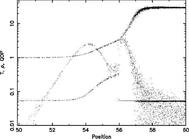
Figure 6: Graph showing the properties of temperature, density and the ratio of the artificial pressure to the pressure for a shock where in-shock cooling has been removed. The temperature starts at $0.054$ and is heated to $0.30$ at position $56$, this temperature being the correct jump temperature. The gas then cools extremely rapidly back down to its upstream value. The density starts at $1$ and increases as the gas shocks and the cools until it reaches its downstream value of $12$. The ratio $q/p$ has a double peaked structure, each peak being caused by shock heating and rapid cooling respectively.

8 Acknowledgments

The authors would like to thank Paul Nulsen for discussion about the effects of in-shock cooling.

References

- [ ] Anninos P., Zhang Y., Abel T. and Norman M. L., New Astronomy, 2, 209
- [ ] Black J.H., 1978, ApJ, 222, 103
- [ ] Chevalier R. A. & Imamura J. N., 1982, ApJ, 261, 543
- [ ] Couchman H., Thomas P. A., and Pearce F. R., 1995, ApJ, 452, 797
- [ ] Haiman Z., Thoul A. A. and Loeb A., 1996, ApJ, 464, 523
- [ ] Hutchins J. B., 1976, ApJ, 205, 103
- [ ] Imamura J.N., Wolff M. T. & Durisen R. H., ApJ, 1984, 276, 667
- [ ] Martin P.G., Schwarz D. H. & Mandy M. E., 1996, ApJ, 461, 265
- [ ] Press W.H., Teukolsky S. A., Vetterling W. T. & Flannery B.P., 1992, Numerical Recepies in Fortran 2nd edition, CUP
- [ ] Raymond J.C. & Smith B. W., Astrophys. J.Suppl., 1977, 35, 419