Non-axisymmetric wind-accretion simulations

Abstract

The hydrodynamics of a variant of classical Bondi-Hoyle-Lyttleton accretion is investigated: a totally absorbing sphere moves at various Mach numbers (3 and 10) relative to a medium, which is taken to be an ideal gas having a density gradient (of 3%, 20% or 100% over one accretion radius) perpendicular to the relative motion. I examine the influence of the Mach number, the adiabatic index, and the strength of the gradient upon the physical behaviour of the flow and the accretion rates of the angular momentum in particular. The hydrodynamics is modeled by the “Piecewise Parabolic Method” (PPM). The resolution in the vicinity of the accretor is increased by multiply nesting several grids around the sphere.

Similarly to the 3D models published previously, both with velocity gradients and without, the models with a density gradient presented here exhibit non-stationary flow patterns, although the Mach cone remains fairly stable. The accretion rates of mass, linear and angular momenta do not fluctuate as strongly as published previously for 2D models. No obvious trend of the dependency of mass accretion rate fluctuations on the density gradient can be discerned. The average specific angular momentum accreted is roughly between zero and 70% of the total angular momentum available in the accretion cylinder in the cases where the average is prograde. Due to the large fluctuations during accretion, the average angular momentum of some models is retrograde by up to 25%. The magnitude is always smaller than the value of a vortex with Kepler velocity around the surface of the accretor.

The models with small density gradients initially display a transient quasi-stable accretion phase in which the specific angular momentum accreted is within 10% of the total angular momentum available in the accretion cylinder. Later, when the flow becomes unstable, the average decreases. I conclude that for accretion from a medium with both density and/or velocity gradients, most of the angular momentum that is available in the accretion cylinder is accreted together with mass. Small gradients hardly influence the average accretion rates as compared to accretion from a homogeneous medium, while very large ones succeed to dominate and form an accretion flow in which the sense of rotation is not inverted.

Table 1: Parameters and some computed quantities for all models. ${\cal M}_{\infty}\equiv{\cal M}_{\infty}(y=0)$ is the Mach number of the unperturbed flow, $\varepsilon_{\rho}$ the parameter specifying the magnitude of the density gradient, $\gamma$ the ratio of specific heats, $t_{\rm f}$ the total time of the run (units: $R_{\rm A}/c_{\infty}$), $\overline{\dot{M}}$ the integral average of the mass accretion rate, $S$ one standard deviation around the mean $\overline{\dot{M}}$ of the mass accretion rate fluctuations, $\widehat{\dot{M}}$ the maximum mass accretion rate, $\dot{M}_{\rm BH}$ is defined in Eq. (3) of Ruffert & Arnett (1994), $l_{\rm x}$, $l_{\rm y}$, $l_{\rm z}$, are the averages of specific angular momentum components together with their respective standard deviations $\sigma_{\rm x}$, $\sigma_{\rm y}$, $\sigma_{\rm z}$, $s$ is the entropy (Eq. (4) in Ruffert & Arnett 1994), the radius of the accretor always is $R_{\star}=0.02R_{\rm A}$, the number of grid nesting depth levels $g=9$, the size of one zone on the finest grid $\delta=1/256R_{\rm A}$, the softening parameter for the potential of the accretor (see Ruffert 1994) $\epsilon=3$ zones, the number $N$ of zones per grid dimension is 32, and the size of the largest grid is $L=32R_{\rm A}$.

Model	${\cal M}_{\infty}$	$\varepsilon_{\rho}$	$\gamma$	$t_{\rm f}$	$\overline{\dot{M}}$	$\!\!\!\!\pm\!\!\!\!$	$S$	$\widehat{\dot{M}}$	$l_{\rm x}$	$\!\!\!\!\pm\!\!\!\!$	$\sigma_{\rm x}$	$l_{\rm y}$	$\!\!\!\!\pm\!\!\!\!$	$\sigma_{\rm y}$	$l_{\rm z}$	$\!\!\!\!\pm\!\!\!\!$	$\sigma_{\rm z}$	$s$
					[$\dot{M}_{\rm BH}$]			[$\dot{M}_{\rm BH}$]	[$\varepsilon_{\rho}R_{\rm A}v_{0}/4$]			[$\varepsilon_{\rho}R_{\rm A}v_{0}/4$]			[$\varepsilon_{\rho}R_{\rm A}v_{0}/4$]			[${\cal R}$]
MV	1.4	0.03	5/3	25.2	0.88	$\!\!\!\!\pm\!\!\!\!$	0.11	0.96	-0.01	$\!\!\!\!\pm\!\!\!\!$	0.01	-0.02	$\!\!\!\!\pm\!\!\!\!$	0.03	+0.76	$\!\!\!\!\pm\!\!\!\!$	0.17	1.14
MS	3	0.03	5/3	10.1	0.62	$\!\!\!\!\pm\!\!\!\!$	0.09	0.77	0.01	$\!\!\!\!\pm\!\!\!\!$	0.50	-0.02	$\!\!\!\!\pm\!\!\!\!$	0.60	+0.38	$\!\!\!\!\pm\!\!\!\!$	1.22	2.8
MF	10	0.03	5/3	4.05	0.45	$\!\!\!\!\pm\!\!\!\!$	0.17	0.69	-0.20	$\!\!\!\!\pm\!\!\!\!$	1.22	+0.52	$\!\!\!\!\pm\!\!\!\!$	3.05	-0.22	$\!\!\!\!\pm\!\!\!\!$	2.36	6.2
NS	3	0.20	5/3	7.96	0.38	$\!\!\!\!\pm\!\!\!\!$	0.09	0.64	-0.09	$\!\!\!\!\pm\!\!\!\!$	0.20	-0.07	$\!\!\!\!\pm\!\!\!\!$	0.26	+0.35	$\!\!\!\!\pm\!\!\!\!$	0.26	2.9
NF	10	0.20	5/3	2.99	0.36	$\!\!\!\!\pm\!\!\!\!$	0.11	0.66	-0.04	$\!\!\!\!\pm\!\!\!\!$	0.20	-0.02	$\!\!\!\!\pm\!\!\!\!$	0.27	+0.40	$\!\!\!\!\pm\!\!\!\!$	0.39	6.0
PS	3	0.03	4/3	9.99	1.03	$\!\!\!\!\pm\!\!\!\!$	0.14	1.43	+0.10	$\!\!\!\!\pm\!\!\!\!$	0.56	-0.23	$\!\!\!\!\pm\!\!\!\!$	0.75	+0.65	$\!\!\!\!\pm\!\!\!\!$	1.94	6.3
PF	10	0.03	4/3	3.99	0.81	$\!\!\!\!\pm\!\!\!\!$	0.15	1.36	-0.19	$\!\!\!\!\pm\!\!\!\!$	1.21	-0.81	$\!\!\!\!\pm\!\!\!\!$	2.51	-0.10	$\!\!\!\!\pm\!\!\!\!$	2.64	13.1
QS	3	0.20	4/3	6.16	0.83	$\!\!\!\!\pm\!\!\!\!$	0.18	1.42	0.00	$\!\!\!\!\pm\!\!\!\!$	0.11	0.00	$\!\!\!\!\pm\!\!\!\!$	0.15	+0.55	$\!\!\!\!\pm\!\!\!\!$	0.26	6.3
QF	10	0.20	4/3	2.21	0.72	$\!\!\!\!\pm\!\!\!\!$	0.10	0.98	-0.01	$\!\!\!\!\pm\!\!\!\!$	0.12	-0.08	$\!\!\!\!\pm\!\!\!\!$	0.20	+0.37	$\!\!\!\!\pm\!\!\!\!$	0.29	12.7
VS	3	1.00	4/3	6.24	0.35	$\!\!\!\!\pm\!\!\!\!$	0.08	0.71	0.00	$\!\!\!\!\pm\!\!\!\!$	0.02	0.02	$\!\!\!\!\pm\!\!\!\!$	0.04	+0.23	$\!\!\!\!\pm\!\!\!\!$	0.04	5.5
TS	3	0.03	1.01	6.14	1.20	$\!\!\!\!\pm\!\!\!\!$	0.10	1.35	-0.02	$\!\!\!\!\pm\!\!\!\!$	0.08	+0.22	$\!\!\!\!\pm\!\!\!\!$	0.54	+1.11	$\!\!\!\!\pm\!\!\!\!$	1.50	68.7
TF	10	0.03	1.01	2.00	0.83	$\!\!\!\!\pm\!\!\!\!$	0.03	0.91	-1.12	$\!\!\!\!\pm\!\!\!\!$	0.08	0.75	$\!\!\!\!\pm\!\!\!\!$	1.11	-0.25	$\!\!\!\!\pm\!\!\!\!$	0.75	201.
US	3	0.20	1.01	6.09	1.19	$\!\!\!\!\pm\!\!\!\!$	0.11	1.43	+0.03	$\!\!\!\!\pm\!\!\!\!$	0.05	+0.08	$\!\!\!\!\pm\!\!\!\!$	0.11	+0.69	$\!\!\!\!\pm\!\!\!\!$	0.23	76.4
UF	10	0.20	1.01	2.22	0.82	$\!\!\!\!\pm\!\!\!\!$	0.04	0.97	-0.14	$\!\!\!\!\pm\!\!\!\!$	0.02	0.16	$\!\!\!\!\pm\!\!\!\!$	0.05	-0.04	$\!\!\!\!\pm\!\!\!\!$	0.07	210.

1 Introduction

The simplicity of the classic Bondi-Hoyle-Lyttleton (BHL) accretion model makes its use attractive in order to estimate roughly accretion rates and drag forces applicable in many different astrophysical contexts. Various aspects of the BHL flow have repeatedly been investigated in the past by many authors. In the BHL scenario a totally absorbing sphere of mass $M$ moves with velocity $v_{\infty}$ relative to a surrounding homogeneous medium of density $\rho_{\infty}$ and sound speed $c_{\infty}$. In this second instalment, I extend the investigations started in Ruffert (1997, henceforth R1) to include density gradients of the surrounding medium. Usually, the accretion rates of various quantities, like mass, angular momentum, etc., including drag forces, are of interest as well as the bulk properties of the flow, (e.g. distribution of matter and velocity, stability, etc.). The results pertaining to total accretion rates tend to agree well qualitatively (to within factors of two, and ignoring the instabilities of the flow) with the original calculations of Bondi, Hoyle and Lyttleton (Hoyle & Lyttleton 1939, 1940a, 1940b, 1940c; Bondi & Hoyle 1944). However, the question of whether and how much angular momentum is accreted together with mass from an inhomogeneous medium has remained largely unanswered, although R1 has attempted a first answer. It has already been summarised in the introduction of R1, that the strict application of the BHL recipe to inhomogeneous media, including some small constant gradient in the density or the velocity distribution, yields that the accreted matter has zero angular momentum by construction (Davies & Pringle, 1980).

We recall that the largest radius $R_{\rm a}$ from which matter is still accreted by the BHL-procedure turns out to be the so-called Hoyle-Lyttleton accretion radius

$$R_{\rm a}=\frac{2GM}{v_{\infty}^{2}}\quad,$$ (1)

where $G$ is the gravitational constant. The mass accretion rate follows to be

$$\dot{M}_{\rm HL}=\pi R^{2}_{\rm a}\rho_{\infty}v_{\infty}\quad.$$ (2)

I will refer to the volume upstream of the accretor from which matter is accreted as accretion cylinder. One can additionally calculate (Dodd & McCrea 1952; Illarionov & Sunyaev 1975; Shapiro & Lightman 1976; Wang 1981) how much angular momentum is present in the accretion cylinder for a non-axisymmetric flow which has a gradient in its density or velocity distribution perpendicular to the mean velocity direction. Then, assuming no redistribution of angular momentum, the amount accreted is equal to (or at least is a large fraction of) the angular momentum present in the accretion cylinder.

The uncertainty about how much angular momentum can actually be accreted in a BHL flow stems from these two opposing views involving either a large or a very small fraction of what is present in the accretion cylinder. In the first paper R1, I showed that the answer is not clear cut, but depends on the initial and boundary conditions. Roughly 7% to 70% of the total angular momentum available in the accretion cylinder is accreted.

Figure 1: The coefficient for the mass accretion rate $f_{\rm m}$ (dotted), defined by Eq. (8), and for the specific angular momentum $f_{\rm j}$ (solid), defined by Eq. (9), as a function of $\varepsilon_{\rho}$. The thin curves show the values of $f$ for a simple linear relation between $v_{{\rm x}\infty}$ and $\varepsilon_{\rho}$, while the bold curves apply to a relation including the “tanh”-term as given in Eq. (4). The two vertical straight lines indicate the gradients that were used in the numerical models (cf. Table 1), $\varepsilon_{\rho}=0.03$ and $\varepsilon_{\rho}=0.2$. Compare this figure with Fig. 1 in paper R1 and note the differences.

In this second paper I would like to compare the accretion rates of the angular momentum of numerically modeled accretion flows with density gradients to the previous results of accretion with velocity gradients (R1). Although several investigations of two-dimensional flows with gradients exist (Anzer et al. 1987; Fryxell & Taam 1988; Taam & Fryxell 1989; Ho et al. 1989; Benensohn et al 1997, Shima et al, 1998), three-dimensional simulations are scarce due to their inherently high computational load. Livio et al. (1986) first attempted a three-dimensional model including gradients, but due to their low numerical resolution the results were only tentative. In the models of Ishii et al. (1993) the accretor was only coarsely resolved, while the results of Boffin (1991) and Sawada et al. (1989) are only indicative, because due to the numerical procedure the flows remained stable (too few SPH particles in Boffin 1991 and local time stepping in Sawada et al. 1989 which was described to be appropriate only for stationary flows). Also Sawada et al. (1989) only investigated velocity gradients.

In order to be able to compare the new results to previous models of R1, I will use the same values for the gradients as in R1. However, as will be mentioned in connection with Eq. 6 (which had already been presented in R1), the expected angular momentum accretion is reduced by a factor of six, when changing from velocity to density gradients. Thus the clear separation between angular momentum from the bulk flow one from the unstable, fluctuating flow blurs. On the other hand arbitrarily large specific angular momenta cannot be accreted because of the ang. mom. barrier felt by matter spiralling into the accretor. A simulation with a very large density gradient was done, too, mainly to be able to compare to a previous 2D model (Fryxell & Taam, 1988).

In Sect. 2 I give an only short summary of the numerical procedure used. Sections 3 and 4 present the results, which I summarise in Sect. 5.

2 Numerical Procedure and Initial Conditions

Since the numerical procedures and initial conditions are mostly identical to what has already been described and used in previous papers (cf. Ruffert 1997, R1, and references therein) I will refrain from repeating every detail, but only give a brief summary.

2.1 Numerical Procedure

The distribution of matter is discretised on multiply nested equidistant Cartesian grids (e.g. Berger & Colella, 1989) with zone size $\delta$ and is evolved using the “Piecewise Parabolic Method” (PPM) of Colella & Woodward (1984). The equation of state is that of a perfect gas with a specific heat ratio $\gamma$ (see Table 1). The model of the maximally accreting, vacuum sphere in a softened gravitational potential is summarised in Ruffert & Arnett (1994) and Ruffert & Anzer (1995).

	Figure 2: Contour plots showing snapshots of the density together with the flow pattern for all models with an adiabatic index of 5/3. The contour lines are spaced logarithmically in intervals of 0.1 dex. The bold contour levels are sometimes labeled with their respective values (0.0, 0.2, and 0.4). Darker shades of gray indicate higher densities. The dashed contour delimits supersonic from subsonic regions. The time of the snapshot together with the velocity scale is given in the legend in the upper right hand corner of each panel.

Figure 3: The accretion rates of several quantities are plotted as a function of time for model MV (${\cal M}_{\infty}$=1.4, gradient of 3%, adiabatic index of $\gamma=5/3$). The left panel contains the mass and angular momentum accretion rates, the right panel the specific angular momentum of the matter that is accreted. In the left panel, the straight horizontal lines show the analytical mass accretion rates: the top solid line is the Bondi-Hoyle approximation formula (Eq. (3) in Ruffert 1994; Bondi 1952) and the lower one half that value. The upper solid bold curve represents the numerically calculated mass accretion rate. The lower three curves of the left panel trace the x (dotted), y (thin solid) and z (bold solid) component of the angular momentum accretion rate. The same components apply to the right panel. The horizontal line in the right panel shows the specific angular momentum value as given by Eq. (7).

Figure 4: The accretion rates of several quantities are plotted as a function of time for the moderately supersonic (${\cal M}_{\infty}$=3) models MS and NS with an index $\gamma=5/3$. The top panels contain the mass and angular momentum accretion rates, the bottom panels the specific angular momentum of the matter that is accreted. In the top panels, the straight horizontal lines show the analytical mass accretion rates: half the value of the Bondi-Hoyle approximation formula (Eq. (3) in Ruffert 1994; Bondi 1952). The upper solid bold curve represents the numerically calculated mass accretion rate. The lower three curves of the top panels trace the x (dotted), y (thin solid) and z (bold solid) component of the angular momentum accretion rate. The same components apply to the bottom panels. The horizontal line in the bottom panels show the specific angular momentum value as given by Eq. (7).

A gravitating, totally absorbing “sphere” moves relative to a medium that has a distribution of density and velocity far upstream (at $x\to-\infty$) given by

$$\rho_{\infty}=\rho_{\rm 0}\left(1-\frac{1}{2}\tanh\left[2\varepsilon_{\rho}\frac{y}{R_{\rm A}}\right]\right)\quad,$$ (3)

$$v_{{\rm x}\infty}=v_{\rm 0}\left(1+\frac{1}{2}\tanh\left[2\varepsilon_{\rm v}\frac{y}{R_{\rm A}}\right]\right),\,\,v_{{\rm y}\infty}=0,\,\,v_{{\rm z}\infty}=0\,\,,$$ (4)

with the redefined accretion radius (note slight difference to Eq. 1)

$$R_{\rm A}=\frac{2GM}{v_{0}^{2}}\quad.$$ (5)

In this paper I only investigate models with gradients of the density distribution, thus for all models I set $\varepsilon_{\rm v}\equiv 0$. The values of $\varepsilon_{\rho}$ can be found in Table 1. In order to keep the pressure constant throughout the upstream boundary, I changed the internal energy or equivalently the sound speed $c$ accordingly ($c^{2}=\gamma p/\rho$). Thus the Mach number ${\cal M}_{\infty}(y)\equiv v/c_{\infty}(y)$ of the incoming flow varies too, since the velocity is kept constant. The Mach numbers given in the Table 1 refer to the values along the axis ($y$=0) upstream of the accretor.

The function “$\tanh$” is introduced in Eq. (3) and (4) to serve as a cutoff at large distances $y$ for large gradients $\varepsilon$. The units I use in this paper are (1) the on-axis sound speed $c_{\infty}(y=0)$ as velocity unit; (2) the accretion radius (Eq. (5)) as unit of length, and (3) the on-axis density $\rho_{0}$ . Thus the unit of time is $R_{\rm A}/c_{\infty}$.

I’ll assume both $\varepsilon_{\rm v}\neq 0$ and $\varepsilon_{\rho}\neq 0$ for the following estimates. Accreting all mass within the accretion cylinder, and taking the matter to have the density and velocity distributions as given by Eqs. (3) and (4) one obtains the mass accretion rate to lowest order in $\varepsilon_{\rm v}$ and $\varepsilon_{\rho}$ to be

$$\dot{M}=\pi R^{2}_{\rm A}\rho_{0}v_{0}\quad,$$ (6)

an equation very similar to Eq. (2). Further assuming that all angular momentum within the deformed accretion cylinder is accreted too, the specific angular momentum of the accreted matter follows to be (Ruffert & Anzer 1994; Shapiro & Lightman 1976; again to lowest order in $\varepsilon_{\rm v}$)

$$j_{\rm z}=\frac{1}{4}\left(6\varepsilon_{\rm v}+\varepsilon_{\rho}\right)v_{0}R_{\rm A}\quad.$$ (7)

For positive $\varepsilon_{\rho}$ the density is lower on the positive side of the $y$-axis, then the vortex formed around the accretor is in the anticlockwise direction, i.e. the angular momentum component in $z$-direction is positive.

The values of the specific angular momentum obtained from the numerical simulations will be compared to the values that follow from this Eq. (7) to conclude which of the above mentioned views — low or high specific angular momentum of the accreted material — is most more appropriate. As was stated further above, R1 found that a sizable amount (between 7% and 70%) is accreted, when velocity gradients are present. I will implicitly assume the component $j_{\rm z}$ when discussing properties like fluctuations, magnitudes, etc. From the symmetry of the boundary conditions the average of the $x$ and $y$ components of the angular momentum should be zero, although their fluctuations can be quite large. Taking the numerically obtained accretion rates of mass $\dot{M}(t)$ and angular momentum $\dot{J}(t)$, I calculate the instantaneous specific angular momentum $j(t)=\dot{J}(t)/\dot{M}(t)$, the temporal mean $l$ of which is listed in Table 1, too.

Apart from serving as cut-off, the tanh-dependencies in Eqs. (3) and (4) have a gradient that is slightly less steep than simply linear. Thus less specific angular momentum is present at a given radius from the accretor and smaller values in the magnitude of the accreted quantity result.

One can numerically approximate the integrals of the mass flux and angular momentum over the cross section of the accretion cylinder, to obtain the coefficients $f$ in the relations Eq. (6) and Eq. (7):

$$\dot{M}=f_{\rm m}(\varepsilon_{\rho})\pi R^{2}_{\rm A}\rho_{0}v_{0}\quad,$$ (8)

$$\jmath_{\rm z}=f_{\rm j}(\varepsilon_{\rho})\varepsilon_{\rho}v_{0}R_{\rm A}\quad.$$ (9)

Here, I will only consider the effect of a density gradient. The unitless functions $f$ are a function of $\varepsilon_{\rho}$ and the functional relation of $\rho_{\infty}[\varepsilon_{\rho}]$, i.e. whether $\rho_{\infty}$ depends purely linearly on $\varepsilon_{\rho}$ or as in Eq. (3) via the “tanh”-term. Figure 1 shows the values of the functions $f$ for the mass and specific angular momentum and for both the linear and “tanh” case. The only minimal deviation of the “tanh” curves from the linear ones indicates that the tanh-cutoff hardly acts within the accretion cylinder. Since $f_{\rm m}\approx 1$ and is practically constant for $\varepsilon_{\rho}\la 1$, Eq. (6) is a good approximation in this range. If the prescription is correct that everything in the accretion cylinder is accreted, no difference in the accretion rate should be observable in the models with differing magnitude of gradient $\varepsilon_{\rho}$ (cf. Table 1). The same constancy applies to the accretion of specific angular momentum: its coefficient $f_{\rm j}$ remains relatively constant $f_{\rm j}\approx 0.25$ in the range $\varepsilon_{\rho}\la 0.4$, which includes both $\varepsilon_{\rho}$ for which models were simulated. So although I used the same magnitudes for the gradients, the effects I expect in the accretion rates are markedly different from what was presented in paper R1. Only for model VS with $\varepsilon_{\rho}=1.0$, does $f_{\rm j}$ deviate appreciably from 0.25: it is $f_{\rm j}\approx 0.16$.

Figure 5: The accretion rates of several quantities are plotted as a function of time for the highly supersonic (${\cal M}_{\infty}$=10) models MF and NF with an adiabatic index of $\gamma=5/3$. The top panels contain the mass and angular momentum accretion rates, the bottom panels the specific angular momentum of the matter that is accreted. In the top panels, the straight horizontal lines show the analytical mass accretion rates: half the value of the Bondi-Hoyle approximation formula (Eq. (3) in Ruffert 1994; Bondi 1952). The upper solid bold curve represents the numerically calculated mass accretion rate. The lower three curves of the top panels trace the x (dotted), y (thin solid) and z (bold solid) component of the angular momentum accretion rate. The same components apply to the bottom panels; the horizontal line shows the specific angular momentum value as given by Eq. (7).

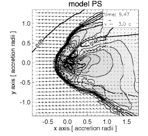
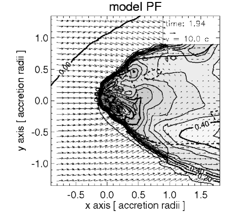
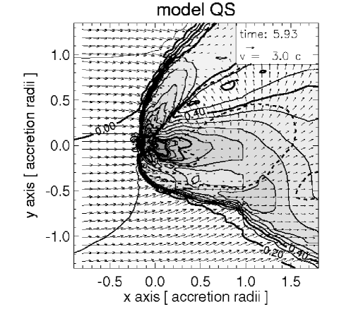
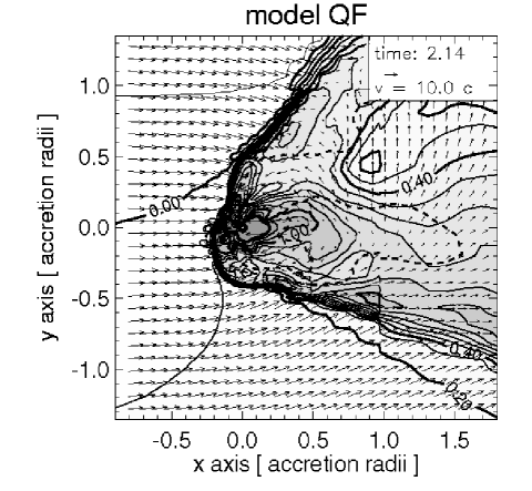
Figure 6: Contour plots showing snapshots of the density together with the flow pattern in a plane containing the centre of the accretor for all models with an adiabatic index of 4/3. The contour lines are spaced logarithmically in intervals of 0.1 dex. The bold contour levels are labeled with their respective values (0.0 or 1.0). Darker shades of gray indicate higher densities. The dashed contour delimits supersonic from subsonic regions. The time of the snapshot together with the velocity scale is given in the legend in the upper right hand corner of each panel.

Figure 7: The accretion rates of several quantities are plotted as a function of time for the moderately supersonic (${\cal M}_{\infty}$=3) models PS and QS with an adiabatic index of $\gamma=4/3$. The top panels contain the mass and angular momentum accretion rates, the bottom panels the specific angular momentum of the matter that is accreted. In the top panels, the straight horizontal lines show the analytical mass accretion rates: dotted is the Hoyle-Lyttleton rate (Eq. (1) in Ruffert 1994), solid is the Bondi-Hoyle approximation formula (Eq. (3) in Ruffert 1994; Bondi 1952) and half that value. The upper solid bold curve represents the numerically calculated mass accretion rate. The lower three curves of the top panels trace the x (dotted), y (thin solid) and z (bold solid) component of the angular momentum accretion rate. The same components apply to the bottom panels; the horizontal line shows the specific angular momentum value as given by Eq. (7).

Figure 8: The accretion rates of several quantities are plotted as a function of time for the highly supersonic (${\cal M}_{\infty}$=10) models PF and QF with an adiabatic index of $\gamma=4/3$. The top panels contain the mass and angular momentum accretion rates, the bottom panels the specific angular momentum of the matter that is accreted. In the top panels, the straight horizontal lines show the analytical mass accretion rates: dotted is the Hoyle-Lyttleton rate (Eq. (1) in Ruffert 1994), solid is the Bondi-Hoyle approximation formula (Eq. (3) in Ruffert 1994; Bondi 1952) and half that value. The upper solid bold curve represents the numerically calculated mass accretion rate. The lower three curves of the top panels trace the x (dotted), y (thin solid) and z (bold solid) component of the angular momentum accretion rate. The same components apply to the bottom panels; the horizontal line shows the specific angular momentum value as given by Eq. (7).

Figure 9: Left panels: The accretion rates of several quantities are plotted as a function of time for the model with largest gradient ($\varepsilon_{\rho}=1.0$). The top panel contains the mass and angular momentum accretion rates, the bottom panels the specific angular momentum of the matter that is accreted. In the top panel, the straight horizontal line shows the analytical half the Bondi-Hoyle value from the approximation formula (Eq. (3) in Ruffert 1994; Bondi 1952). The upper solid bold curve represents the numerically calculated mass accretion rate. The lower three curves of the top panel trace the x (dotted), y (thin solid) and z (bold solid) component of the angular momentum accretion rate. The same components apply to the bottom panel. Right panel: Comparison of the ratio of specific angular momenta accreted for models with density gradients (MS, MF, PS, NS, NF) to models with velocity gradients (IS, JS, SS, KS, LS taken from paper R1), keeping all other parameters equal.

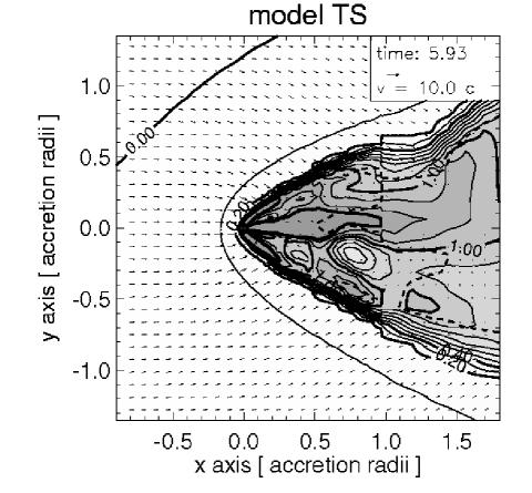
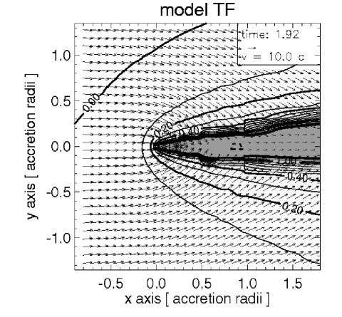
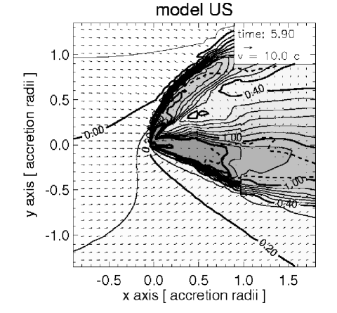
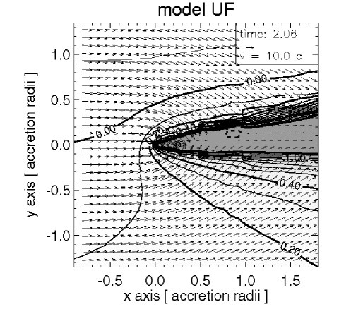
Figure 10: Contour plots showing snapshots of the density together with the flow pattern in a plane containing the centre of the accretor for all models with an adiabatic index of 1.01 The contour lines are spaced logarithmically in intervals of 0.1 dex. The bold contour levels are labeled with their respective values (0.0 or 1.0). Darker shades of gray indicate higher densities. The dashed contour delimits supersonic from subsonic regions. The time of the snapshot together with the velocity scale is given in the legend in the upper right hand corner of each panel.

Figure 11: The accretion rates of several quantities are plotted as a function of time for the moderately supersonic (${\cal M}_{\infty}$=3) models TS and US with an adiabatic index of $\gamma=1.01$. The top panels contain the mass and angular momentum accretion rates, the bottom panels the specific angular momentum of the matter that is accreted. In the top panels, the straight horizontal lines show the analytical mass accretion rates: dotted is the Hoyle-Lyttleton rate (Eq. (1) in Ruffert 1994), solid is the Bondi-Hoyle approximation formula (Eq. (3) in Ruffert 1994; Bondi 1952) and half that value. The upper solid bold curve represents the numerically calculated mass accretion rate. The lower three curves of the top panels trace the x (dotted), y (thin solid) and z (bold solid) component of the angular momentum accretion rate. The same components apply to the bottom panels; the horizontal line shows the specific angular momentum value as given by Eq. (7).

Figure 12: The accretion rates of several quantities are plotted as a function of time for the highly supersonic (${\cal M}_{\infty}$=10) models TF and UF with an adiabatic index of $\gamma=1.01$. The top panels contain the mass and angular momentum accretion rates, the bottom panels the specific angular momentum of the matter that is accreted. In the top panels, the straight horizontal lines show the analytical mass accretion rates: dotted is the Hoyle-Lyttleton rate (Eq. (1) in Ruffert 1994), solid is the Bondi-Hoyle approximation formula (Eq. (3) in Ruffert 1994; Bondi 1952) and half that value. The upper solid bold curve represents the numerically calculated mass accretion rate. The lower three curves of the top panels trace the x (dotted), y (thin solid) and z (bold solid) component of the angular momentum accretion rate. The same components apply to the bottom panels. The horizontal line in the bottom panels show the specific angular momentum value as given by Eq. (7).

2.2 Models

The combination of parameters that I varied, together with some results are summarised in Table 1. The first letter in the model designation indicates the strength of the gradient: M, P, and T have $\varepsilon_{\rho}=0.03$, while N, Q, and U have $\varepsilon_{\rho}=0.2$ and V is $\varepsilon_{\rho}=1.0$. The second letter specifies the relative wind flow speeds, F (fast), S (slow) and V stand for Mach numbers of 10, 3 and 1.4, respectively. I basically simulated models with all possible combinations of the two higher flow speeds (Mach numbers of 3 and 10), the two gradients (3% and 20%) and varying the adiabatic index between 5/3, 4/3 and 1.01. Model VS with the largest gradient of 100% facilitates a comparison to a previous two-dimensional simulation by Fryxell & Taam (1988). The grids are nested to a depth $g=9$ such that the radius of the accretor $R_{\star}=0.02R_{\rm A}$ spans several zones on the finest grid.

As far as computer resources permitted, I aimed at evolving the models for at least as long as it takes the flow to move from the boundary to the position of the accretor which is at the centre (crossing time scale). This time is given by $L/2{\cal M}_{\infty}$ and ranges from about 1 to about 10 time units. The actual time $t_{\rm f}$ that the model is run can be found in Table 1, as well as the parameters of the grids ($L$, $g$, etc.).

When modeling a BHL flow with a density gradient, one has to pay attention to the fact that matter parcels with possibly very different densities (which initially are separated upstream) will be focussed to find themselves close to each other along the accretion axis (U. Anzer, personal communication). This might render the flow additionally unstable. Although true in principle, this problem does not affect, in practice, the models I will present: a closer inspection of Eq. (3) reveals that the density jump from one end of the accretion radius to the other is only a factor 1.5 for the case with large gradient ($\varepsilon=0.2$). This does not seem to have an additional influence as compared to models with constant density presented in paper R1.

The calculations are performed on a Cray-YMP 4/64 and a Cray J90 8/512. They need about 12–16 MWords of main memory and take approximately 160 CPU-hours per simulated time unit.

Figure 13: Mass accretion rates (units: $\dot{M}_{\rm BH}$) are shown as a function of the strength of the density gradient: the points to the right of lg gradient = -2 are the results from this work, while the values for models without gradient (at the x-axis position “-infty”) are taken from Ruffert (1994) and Ruffert & Arnett (1994). Diamonds ($\Diamond$) denote models in which $\gamma=5/3$, triangles ($\triangle$) models with $\gamma=4/3$, and squares ($\Box$) show $\gamma=1.01$ The large bold symbols belong to models with a speed of ${\cal M}_{\infty}=10$, while the smaller symbols belong to models with ${\cal M}_{\infty}=3$. The adiabatic index $\gamma$ and Mach number are also written near each set of points. The “error bars” extending from the symbols indicate one standard deviation from the mean ($S$ in Table 1). Some points were slightly shifted horizontally to be able to discern the error bars.	Figure 14: The relative mass fluctuations, i.e.  the standard deviation $S$ divided by the average mass accretion rate $\overline{\dot{M}}$ (cf. Table 1), is shown as a function of the strength of the density gradient: 20% and 3% are the results from this work, while the values for models without gradient (at the x-axis position “-infty”) are taken from Ruffert (1994) and Ruffert & Arnett (1994). Diamonds ($\Diamond$) denote models in which $\gamma=5/3$, triangles ($\triangle$) models with $\gamma=4/3$, and squares ($\Box$) show $\gamma=1.01$ The large bold symbols belong to models with a speed of ${\cal M}_{\infty}=10$, while the smaller symbols belong to models with ${\cal M}_{\infty}=3$.
Figure 15: The average accreted specific angular momentum (units: $l_{\rm s}$, Kepler velocity vortex at surface of accretor, as given by Eq. (10) in R1) is shown for most models by diamond symbols ($l_{\rm z}$ in Table 1). The “error bars” extending from the symbols indicate one standard deviation from the mean ($\sigma_{\rm z}$ in Table 1). The long error bars extending to the bottom axis are an indication that the fluctuations of the respective model are so large, that the specific angular momentum changes sign from time to time. The plus signs above the diamonds indicate the specific angular momentum $j_{\rm z}$ according to Eq. (7).	Figure 16: The mass accretion rate is plotted versus the specific angular momentum of the accreted matter for model QS. Each dot displays the two quantities at one moment in time. Only dots at time later than $t\ga 0.8$ are plotted to avoid the initial transients.

3 Dynamics and accretion rates

3.1 Results of models with $\gamma$=5/3 and 4/3

I will describe the results of the models for which a ratio of specific heats of $\gamma$=5/3 was chosen together with those models of $\gamma$=4/3 because the evolution is very similar. The only exception is model MV: its slow relative bulk velocity of Mach 1.4 produces a significantly more stable flow.

Figs. 2 and 6 show snapshots of the flow velocities and density distribution in the x-y-plane containing the accretor. The velocity pattern as well as the density contours within the shock cone indicate a strongly unstable flow. Also the shock cone itself has many bumps and kinks.

Note how the density contours strongly bend over upstream of the shock (at $x\approx-0.8$) for models N and Q indicating the large gradient as compared to models M and P, where only the contour of $\rho=1$ is seen to be detached from the shock. The higher densities on the lower side of $y$ (where it is negative) seem to produce an asymmetric shock cone: the lower part of the cone subtends a smaller angle with the $y=0$-axis than the upper half. However, the quickly varying accretion flow pattern tends to impinge on the shock front and dislodge it. This asymetry has been observed and commented on in Ishii et al. (1993) and Soker & Livio (1984). In the models with smaller $\gamma$ (models P and Q) the shock cone tends to be narrower and its minimum distance from the accretor smaller than for the models M and N.

In contrast to what has been said, model MV with a slow (but still supersonic relative velocity), shows a very regular flow pattern: the stagnation point is about 0.3 $R_{\rm A}$ downstream from the accretor. Matter that comes within this point gets accreted while matter that stays outside just passes the accretor. The mass accretion rate of model MV (cf. Fig. 3) rises slowly and nearly monotonically to saturate close to the Bondi-Hoyle formula value. Only towards the end is there an indication that the flow might become unstable for this model too. The component of interest ($z$) for the specific angular momentum saturates at about 75% of the value estimated analytically by Eq. (7). This is probably due to the fact that for bulk velocities close to a Mach number of unity the Hoyle-Lyttleton approximation brakes down because a certain fraction of mass is accreted practically spherically symmetrically, i.e. as Bondi tried to describe it with the approximative formula (Bondi, 1952). The other two components ($x$ and $y$) fluctuate around zero (which is given by the symmetry of the boundary conditions), but indicate at a very early stage that the flow is mildly unstable.

The other 8 models (MS, MF, NS, NF, PS, PF, QS, QF) show very strong fluctuations of the accretion rates of mass and all angular momentum components (Figs. 4, 5, 7, and 8). A variation of factors of two is not uncommon, so the averages stated in Table 1 should be used with care and where possible the standard deviations taken into account. I include the accretion rate plots for all models in order to facilitate the judgement of how representative the average values are for the whole temporal evolution.

A few trends can be discerned. All four models MS, MF, PS, PF, i.e. the ones with small $\varepsilon_{\rho}=0.03$ display a fairly quiet initial transient phase. The $x$ and $y$-components of the angular momentum fluctuate mildly around zero and the $z$-component reaches fairly precisely (to within 10%) the analytic estimate Eq. (7). This shows the applicability of the analytic result only to the initial quasi-stationary state. The models with large $\varepsilon_{\rho}=0.2$ do not have this quiet phase but become chaotic much quicker. This decreased stability also produces lower accretion rates for mass as well as lower specific angular momenta. The initial quiet transient phase has already been seen in R1: compare the present models to the ones from R1, IS, JS, KS, LS in Figs. 4, 6, 8, and 9 in R1, respectively.

Note that model PF is one for which the simulation was run fairly long compared to the timescale of fluctuations. This increases the confidence that the average mass accretion rate is a representative value and not a random one of a transient state. The angular momenta, however, still do not display the marginal positive shift that the z-component should have compared to the other two.

No significant difference is observed when comparing two models that only differ in Mach number. However the mass accretion rates are significantly larger in the models with smaller $\gamma$, again ceteris paribus. The same applied to the velocity gradient models of R1, cf. model IS and SS in Figs. 4 and 11 respectively. This dependence of the accretion rate on the adiabatic index $\gamma$ is well known for stationary flows from analytic calculations, e.g. Bondi (1952) for spherically symmetric flows and Sect. 5 and 6 and Figs. 9 and 10 in Foglizzo & Ruffert (1997).

3.2 Results of models with $\gamma$=1.01

The first main obvious difference between the nearly isothermal models and the more adiabatic ones is that the shock cone is attached to the accretor, as can be seen in Fig. 10. The pressure around the accretor in this case is not sufficient to push away and support the shock cone. Not even the large density gradient is able to dislodge the shock from touching the surface of the accretor.

Both models with high Mach number (TF and UF) hardly show any activity of unstable flow within the shock cone, contrary to the moderately supersonic cases (TS and US). Again (as in model MV) a clear and stable stagnation point is present downstream of the accretor for these quiet models. It is a common feature of practically all simulations (including the ones by other authors) that when the shock cone is attached to the accretor no (or hardly any) instability is observed. Whether or not the shock cone is attached depends on many physical attributes of the models (e.g. stiffness of the equation of state, etc.) and numerical parameters (not least resolution). However, when these conditions collude to produce an attached shock, invariably the flow remains stable.

The very active flow of the slower models (TS and US) reflects itself in a higher variability of the mass accretion rate as compared to models TF and UF (Figs. 11 and 12). However the fluctuation of the mass accretion rates of all these $\gamma=1.01$ models is much smaller than the fluctuations shown by the more adiabatic models described further above. The average mass accretion rates of the slow models slightly exceed the values predicted by the Hoyle-Lyttleton theory, while the faster models only reach 80% of $\dot{M}_{\rm BH}$. The $z$-component of the specific angular momentum in the models with large gradient (US, UF) practically never reach the analytical estimate Eq. (7) while the models with small gradient (TS, TF) fluctuate strongly about this value, exceeding it by a factor of three or even reversing sign.

These models can be compared to models without gradients (Ruffert, 1996) but with the same remaining parameters: models TF and UF should be compared to model HS in Fig. 7e, while models TS and US can be compared to model GS in Fig. 5e of Ruffert (1996). Both the different behaviour of the mass accretion rates as well as the amplitudes of fluctuation of the angular momentum accretion rates are comparable between the models, indicating that the presence of a density gradient does not significantly alter the accretion properties of such a strongly unstable flow. Of course, the mean of the $z$-component is not zero in flows with gradients. Fig. 11 can also directly be compared with Fig. 11 from Ishii et al. (1993). Both the mass and angular momentum accretion rates show very similar magnitudes and evolution.

3.3 Results of model VS

The density gradient in the previous set of models of $\varepsilon_{\rho}=0.03$ and $\varepsilon_{\rho}=0.2$ was chosen in order to facilitate the direct comparison between the results presented in this paper and the ones with velocity gradients shown in R1. However, Eq. 7 then predicts that the specific angular momentum accreted will be six times smaller for the density gradients as compared to accretion with velocity gradients. That this is true becomes clear when comparing the plots for models MS, MF, PS, NS and NF with equivalent models from paper R1: IS, JS, SS, KS and LS, respectively: In the models presented in this paper, the z-component of the angular momentum, which is the one influenced by the gradient, hardly rises above the random fluctuations of the other two components. In order to check the correct separation of the effect of the density gradient from the unstable nature of the flow, a model with larger gradient is helpful and will be presented in this subsection.

The particular value of $\varepsilon_{\rho}=1$ is suggested because for this case, Taam & Fryxell (1988) have found that a quasi-steady disk forms which does not change its sense of direction. Fig. 9 (left panels) shows the temporal evolution of the mass and angular momentum accretion for this large density model. The mass accretion rate remains very low over the whole simulated time on average being less than half the value of model QS (which is similar to VS in all parameters except $\varepsilon_{\rho}$). Note that these average values listed in Table 1 are normalised to Eq. 7 and not to Eq. 9. Thus a big part of the reduction of specific angular momentum between model QS (0.55) and model VS (0.23) is probably due to the “tanh”-term represented by the factor $f_{j}$ (Fig. 1): $f_{j}\approx 0.25$ for model QS while $f_{j}\approx 0.16$ for model VS.

Also note that model VS does not display as drastic a reduction in mass accretion rate as shown in Fig. 22 of Taam & Fryxell (1988) [note the different choice of time units between this paper and the one in Taam & Fryxell, 1988]. The reason probably being that in their 2D models accretion gets effectively shut off as soon as a stable disk structure forms, while in my 3D simulations accretion can still proceed practically unimpeded via the poles.

The lower left panel of Fig. 9 shows the angular momentum accretion. In this large gradient model, the z-component clearly dominates compared to the other two components, i.e. the fluctuating flow cannot compete with the angular momentum available in the bulk flow gradient. Note also that the z-component never crosses the $y=0$ line which indicates the formation of a disk-like flow structure with rotation in an unchanging sense. However, I do not expect the specific angular momentum to reach a quasi-steady state because of the three-dimensional nature of my simulations: angular momentum can continue to be accreted from directions outside the plane of the disk and thus probably disturbing the disk, too.

4 Comparison of accretion rates

4.1 Mass accretion rates

I collected all the means of the mass accretion rates and their standard deviation into Fig. 16 together with the appropriate values for models without gradients. The standard deviation is shown as “error bar” in order to give an indication on how precisely one should interpret the mean values.

(a) The mass accretion rates are fairly independent of the density gradient strength for small $\gamma$, but a decrease of the rates might be present when increasing the gradients: a slight trend toward smaller rates for larger gradients seems possible. (b) A clear increase of the rates is visible when decreasing the index $\gamma$. When going from 5/3 to 1.01 the accretion rate increases by over a factor of two. (c) Models with smaller Mach numbers have larger rates. This trend also applies to models with a velocity gradient as can be seen in Fig. 12 of R1.

Because the fluctuations of the mass accretion rate slightly decrease with decreasing $\gamma$, while at the same time the rate itself increases, it follows that the relative fluctuation decreases strongly with decreasing $\gamma$ as can be seen in Fig. 16. No obvious trend seems visible on how the relative fluctuations change with gradient strength; a slight increase might be present when comparing the larger gradient fluctuation with the smaller gradient ones.

The dependence of the relative fluctuations on velocity seems to invert: while they are clearly larger for smaller Mach numbers for the $\gamma=1.01$ models, they are smaller for smaller Mach numbers in the $\gamma=5/3$ models. And last, the simulations with $\gamma=4/3$ produce relative fluctuations that vary more strongly with gradient strength than with Mach number.

4.2 Specific angular momentum

As has already been described in Sect. 3 the specific angular momentum reaches the analytic values given by Eq. (7) to within 10%, but only as long as the accretion flow is roughly stable and only for the models with small density gradients, $\varepsilon_{\rho}=0.03$. In Fig. 16 I show the specific angular momentum averaged over the whole time the models were evolved, excluding the initial transients. This gives a better picture of how the very unstable flow tends to decrease the average and produce a large fluctuation of the specific angular momentum. So I included as “error bars” the standard deviation of the fluctuations around the mean.

The unit I chose in Fig. 16 is the specific angular momentum that a vortex just at the surface of the accretor would have if it spun with the local Kepler velocity. Thus unity in these units indicates a Kepler orbit and matter that has more specific angular momentum than this would be flung off. One can see in Fig. 16 that the matter accreted is well below this value. For comparison, I also plot, using plus signs (+), the specific angular momentum as given by Eq. (7). These values tend to lie above the mean, especially for the models with large gradients (N,Q,U), and are well within one standard deviation from the mean for the small gradient models (M,P,T). For the latter models the fluctuations are so large that occasionally the sign of the accreted specific angular momentum reverses; this is indicated by the “error bars” extending completely down to the $x$-axis.

If one is only interested in the average specific angular momentum that is accreted, an inspection of Table 1 yields that the whole range of values between zero and about 70% is attained depending on the model parameters. Livio et al. (1986) reported values between 10% and 20% for their parameters.

If one reduces the size of the accretor, some point will be reached when the maximum specific angular momentum that can be accreted will become smaller than the amount present in the accretion cylinder. Setting Eq. (7) equal to Eq.(10) in R1 a relation is obtained between the gradients in the flow ($\varepsilon$) and the radius of the accretor $R_{\star}$:

$$R_{\star}=\frac{1}{32}(6\varepsilon_{\rm v}+\varepsilon_{\rho})^{2}R_{\rm A}\quad.$$ (10)

So for accretors smaller than this radius the angular momentum accretion should no longer be dominated by what is given in the accretion cylinder. For $\varepsilon_{\rm v}$=0 and $\varepsilon_{\rho}$=0.03 and 0.2 we obtain $R_{\star}\approx 3\cdot 10^{-5}R_{\rm A}$ and $R_{\star}\approx 10^{-3}R_{\rm A}$. Both these values are below what is currently possible to simulate numerically, but could be important in astrophysical objects. On the other hand for model VS, which has $\varepsilon_{\rm v}$=0 and $\varepsilon_{\rho}$=1.0, an accretor radius of $0.03R_{\rm A}$ results, which is larger than the numerically used radius of $0.02R_{\rm A}$. Thus in model VS not all the specific angular momentum offered in the incoming bulk flow can be accreted. Vice-versa, the maximum gradient $\varepsilon$ that can be accommodated by an accretor of given radius $R_{\star}$ is

$$\varepsilon^{\rm max}_{\rho}=\sqrt{32\frac{R_{\star}}{R_{\rm A}}}\quad\quad\quad\quad\varepsilon^{\rm max}_{\rm v}=\sqrt{\frac{16}{3}\frac{R_{\star}}{R_{\rm A}}}$$ (11)

The right panel of Fig. 9 compares the specific angular momentum accreted between the density gradient models presented here and the velocity gradient models shown in R1. The ratio (cf. legend of the x-axis of Fig. 9) is plotted of the specific angular momentum (values given in Table 1) for these two sets of models. If a pair of models experiences the same reduction in accretion of specific angular momentum, the ratio plotted would be one. If the density-gradient model of the pair suffers a greater decrease of accretion (due to e.g. stronger relative fluctuations of the unstable flow) this will be reflected by a ratio that is smaller than unity.

The pair MF/JS is less than zero, because the average angular momentum accreted by model MF is actually retrograde to the bulk flow momentum. For this pair, as well as for MS/IS, the very large ’error’ bar indicates that the fluctuations due to the unstable flow are very large compared to the average and so the latter value does not permit a strong statement. So although for four of the five models the ratios are above unity, which would indicate that the unstable flow actually increases the angular momentum accretion for the density gradient models as compared to the velocity gradient models, this reasoning is not a credible one. Additionally one has to keep in mind that the specific angular momentum of the incoming bulk flow of models KS and LS is actually larger than the maximum permitted by the Eq. 11. Thus the accreted momentum will be decreased due to this effect, too (angular momentum barrier), which explains why these model-pairs have the largest ratios.

4.3 Correlations

A correlation was found in R1 (Fig. 17) between the mass accretion rate and the specific angular momentum: the rate decreases when the magnitude of the momentum is largest. In Fig. 16 I draw a similar plot as in R1, each dot connecting the two quantities for every second timestep of the numerical simulation. A similar trend can be seen for model QS, which confirms that the dynamics is similar: when the flow does not rotate (low specific angular momentum) if falls down the potential to the surface of the accretor and thus produces a higher mass accretion rate. For all other models a correlation is not obvious.

5 Summary

For the first time a comprehensive numerical three-dimensional study is presented of wind-accretion with a density gradient using a high resolution hydrodynamic code. I vary the following parameters: Mach number of the relative flow (Mach ${\cal M}$=3 and 10), strength of the density gradient perpendicular to this flow ($\varepsilon_{\rho}$=3%, 20% and 100% over one accretion radius), and adiabatic index ($\gamma$=5/3, 4/3, and 1.01). The results are compared (a) among the models with different parameters, (b) to some previously published simulations of models with density and velocity gradients, and (c) also to the analytic estimates of the specific angular momentum.

1. All models exhibit active unstable phases, which are very similar to the models without gradients. Only the mildly supersonic case (${\cal M}$=1.4) displayed a relatively steady flow (as compared to the faster flow models). The accretion rates of mass, linear and angular momentum fluctuate with time, although not as strongly as published previously for 2D models.

2. Depending on the model parameters, the average specific angular momentum accreted is roughly between zero and 70% of the analytical estimate, which assumes that all angular momentum within the accretion cylinder is actually accreted.

3. The mass accretion rates of all models with density gradients are equal, to within the fluctuation amplitudes, to the rates of the models without gradients (published previously), although the accretion rates might seem to decrease slightly when increasing the density gradient. The fluctuations of the mass accretion rate in all models hardly vary with gradient strength.

4. The overall qualitative flow dynamics as well as the mass accretion rates are very similar to what has been published on models with velocity gradients. Of course the accretion rate of angular momentum and its specific values (i.e per mass unit) are reduced if one compares equal gradients for both velocity and density, well in accordance with the analytic estimates. This reduction means that in the density gradient models the fluctuations due to the unstable accretion flow have a greater influence on the angular momentum accretion than for the velocity gradient models.

5. The models with small gradients ($\varepsilon_{\rho}$=0.03) display an initially quiet stable phase, in which the specific angular momentum of the matter accreted is within 10% of the analytic estimate. Thus for the quiescent phases the analytic values are appropriate. The average drops when the flow becomes unstable.

6. The model with very large density gradient ($\varepsilon_{\rho}=100\%$ over one accretion radius) was the only one for which the accreted angular momentum was always prograde with respect to the angular momentum available in the incoming flow. Here the amplitude of the perturbation due to the unstable flow is much smaller than the average angular momentum accreted. However the specific angular momentum of the incoming flow in this case is larger than the maximum given by the Kepler velocity times the radius of the accretor surface.