On the enigmatic X-ray Source V1408 Aql (=4U 1957+11)

Abstract

Models for the characteristically soft X-ray spectrum of the compact X-ray source V1408 Aql (=4U 1957+11) have ranged from optically thick Comptonization to multicolor accretion disk models. We critically examine the X-ray spectrum of V1408 Aql via archival Advanced Satellite for Cosmology and Astrophysics (ASCA) data, archival Röntgensatellit (ROSAT) data, and recent Rossi X-Ray Timing Explorer (RXTE) data. Although we are able to fit a variety of X-ray spectral models to these data, we favor an interpretation of the X-ray spectrum as being due to an accretion disk viewed at large inclination angles. Evidence for this hypothesis includes long term (117 day, 235 day, 352 day) periodicities seen by the RXTE All Sky Monitor (ASM), which we interpret as being due to a warped precessing disk, and a 1 keV feature in the ASCA data, which we interpret as being the blend of L fluorescence features from a disk atmosphere or wind. We also present timing analysis of the RXTE data and find upper limits of 4% for the root mean square (rms) variability between f=$10^{-3}-16$ Hz. The situation of whether the compact object is a black hole or neutron star is still ambiguous; however, it now seems more likely that an X-ray emitting, warped accretion disk is an important component of this system.

1. Introduction

The low mass X-ray binary (LMXB) V1408 Aql ($=$4U 1957+11, 3U 1956+11) was detected during scans of the Aquila region by Uhuru in 1973 (Giacconi et al. (1974)), and it was subsequently identified with an 18$\fm$7 star having a strong blue excess (Margon, Thornstensen & Bowyer (1978)). The object is situated in a region of relatively small extinction ($N_{\rm H}\approx 1.3\times 10^{21}\,{\rm cm^{-2}}$; Dickey & Lockman (1990); Stark et al. (1992)). $A_{\rm V}$ measurements place the source at a distance $>$2.5 kpc, and comparisons of its X-ray and optical luminosity to Sco X-1 place it at a distance of $\sim$7 kpc (Margon, Thornstensen & Bowyer (1978)).

Little is known about the nature of the system. Optical spectra of V1408 Aql reveal a power-law continuum with H$\alpha$, H$\beta$, and He ii 4686Å emission lines (Cowley, Hutchings & Crampton (1988); Shahbaz et al. (1996)), typical for an accretion disk-dominated system. Thorstensen (1987) reported a nearly perfectly sinusoidal V-band luminosity modulation with 10% amplitude and a 0.389 d (=9.33 h) period, which he interpreted as due to X-ray heating of the companion. In recent multicolor photometry a more complex lightcurve with 30% modulation amplitude was observed. Hakala, Muhli & Dubus (1999) interpret this change in the shape of the lightcurve as evidence for a disk with a large outer rim, possibly due to a warped disk, seen close to edge on (Hakala, Muhli & Dubus (1999); see also §4). This interpretation is also consistent with the shape of the infrared spectrum (Smith, Beall & Swain (1990)). The short orbital period is indicative of a late type main sequence star of $M\sim 1\,{\rm M}_{\odot}$ as the donor star. The absence of X-ray eclipses and the assumption that the donor star fills its Roche lobe yield an upper limit on the orbital inclination of $i\sim 70^{\circ}$–$75^{\circ}$, consistent with the models for the optical variability (Hakala, Muhli & Dubus (1999)).

V1408 Aql is one of the less well-studied possible black hole candidates (BHCs). Identification as either a BHC or a neutron star-low mass X-ray binary (NS-LMXB) is usually made by analogy with the spectral- and timing-behavior of better observed sources. V1408 Aql has been a BHC since 1984, when EXOSAT X-ray observations revealed that V1408 Aql has a very soft X-ray spectrum, similar to that of other BHC. In color-color-diagrams, V1408 Aql lies halfway between the black hole candidate GX 339$-$4 (in its high/soft state) and the neutron-star LMXBs Cyg X-2 and LMC X-2 (White & Marshall (1984); Schulz, Hasinger & Trümper (1989)). This color identification of V1408 Aql as a BHC, however, is not definitive.

Previous narrow-band observations have not characterized the X-ray spectrum in a consistent manner. The analysis of 1983 and 1985 EXOSAT observations of V1408 Aql led to contradictory results. While Singh, Apparao & Kraft (1994) succeeded in fitting a Comptonization spectrum to these data and interpreted this as an indication that V1408 Aql is a black hole candidate, Ricci, Israel & Stella (1995) interpreted the same data as being similar to that observed from NS-LMXBs. Observations with Ginga, with its larger spectral range and effective area, have shed more light on the nature of V1408 Aql (Yaqoob, Ebisawa & Mitsuda (1993)). The values of the normalizations of multicolor disk models (MCD; Mitsuda et al. (1984)), i.e. $(r_{\rm in}/d)^{2}\cos i$ where $r_{\rm in}$ is the inner disk radius, $d$ is the distance to the source, and $i$ is the inclination, have been used to distinguish between BHCs and NS-LMXBs (Tanaka & Lewin (1995)). In the case of V1408 Aql, $r_{\rm in}\cos^{1/2}i\approx 2~{}{\rm km}$ assuming $d=7$ kpc, which is more characteristic of sources containing neutron stars. Additionally, the Ginga observation showed evidence of a hard tail (1–18 keV) comprising $\sim 25\%$ of the inferred flux for this system at that time. The best fit power-law photon indices for the hard component ranged from $\Gamma\approx 2$ to $3$.

The EXOSAT observations of Ricci, Israel & Stella (1995) indicate the presence of an iron fluorescence line with an equivalent width of 90 eV or smaller and a line-energy of 7.06 keV (i.e., highly ionized). Other values in the literature range from non-detection (e.g., Yaqoob, Ebisawa & Mitsuda (1993)) to 200 eV (White & Marshall (1984)), the uncertainty being mainly due to the difference in the assumed spectral continua and the different sensitivities of the instruments.

Except for one observation, which hints toward a weak red-noise ($f^{-\alpha}$) component between $10^{-4}$ and $10^{-3}$ Hz, all EXOSAT observations are consistent with the absence of any periodic features (Ricci, Israel & Stella (1995)). The Ginga observations have yet to have their short timescale variability analyzed; however, they do show evidence of significant flux and color changes on long time scales ($\gtrsim 10^{4}$ s). The Vela 5B satellite did not detect any long-term X-ray variability from this source (Priedhorsky & Terrell (1984)); however, the upper limits to the variability were not particularly strong.

If the published spectral models are accepted at face value, then the relative energetics of the disk black-body and power-law components, as well as the slope of the high-energy power-law, are very similar to those seen in BHCs such as LMC X-1 (Ebisawa, Mitsuda & Inoue (1989); Wilms et al. (1998b)), LMC X-3 (Treves et al. (1988); Wilms et al. (1998b)), and in the soft state of GX 339$-$4 (Miyamoto et al. (1991); Grebenev et al. (1991)). However, at luminosities as low as that of V1408 Aql, BHCs tend to show hard tails with no evidence of a disk or thermal component. On the other hand, NS-LMXBs that exhibit soft disk spectra also tend to show an additional $\sim 2$ keV blackbody component, while showing little hard flux (Miyamoto (1994), and references therein). Furthermore, low-luminosity NS-LMXBs also tend to be dominated by hard emission.

Thus, there are good arguments that point towards V1408 Aql being a neutron star and also toward it being a black hole; however, none of the arguments are truly conclusive. In either case, V1408 Aql would still be a unique object, being either an unusually soft low-luminosity BHC, an unusually soft low-luminosity neutron star, or a soft neutron star with an unusually energetic hard tail. With the advent of X-ray detectors with much larger effective areas than EXOSAT and Ginga, as well as with the availability of detectors of higher energy resolution, such as those on the Advanced Satellite for Cosmology and Astrophysics (ASCA), a critical reexamination of the X-ray spectrum of V1408 Aql has become possible. In this paper we present the results from our analysis of a 30 ksec pointed observation with the Rossi X-Ray Timing Explorer (RXTE), as well as archival data from ASCA and the Röntgensatellit (ROSAT). In §2 we present the results from the spectral analysis. We discuss the timing analysis in §3, the long term variability of the source in §4, and we discuss our results in §5. The details of the data extraction are described in an appendix.

Table 1Observing log for V1408 Aql. Count rates given are background subtracted.

Date	On-Source Time	Instrument	Count Rate
	[ksec]		[cps]
1997 November 26.02–26.45	21.2	RXTE-PCA	230
1997 November 27.08–27.17	4.7		229
1997 November 29.08–29.15	1.5		233
1994 October 31.13–31.93	21.6	ASCA SIS0	9.8
		ASCA SIS1	7.0
		ASCA GIS2	19.4
		ASCA GIS3	21.5
1992 May 08.39–11.14	14.6	ROSAT PSPC	19.2

2. Spectral Analysis

V1408 Aql was observed with RXTE in 1997 November in three observing blocks for a total on source time of 27 ksec. A log of the observations is given in Table 1. Since the spectral shapes of the three observing blocks are identical, the data were analyzed together. Spectral and temporal data were extracted using the methods outlined in appendix A.1. Spectral analysis was performed with XSPEC, version 10.0s (Arnaud (1996)).

The RXTE spectrum of V1408 Aql is very soft. The Proportional Counter Array (PCA) did not detect any flux above $\sim$20 keV and the High Energy X-ray Timing Experiment (HEXTE) count rates are consistent with zero: the background subtracted count rates were $0.4\pm 0.2$ cps and $0.0\pm 0.2$ cps, for HEXTE clusters A and B, respectively. The residual flux in cluster A is most probably due to a slight overestimation of the HEXTE background dead time, as the spectrum seen is similar to the HEXTE background. Therefore, we do not consider V1408 Aql to be detected with HEXTE and will not further discuss these data.

Table 2Results of spectral fitting

Model	Detector	Parameters			$\chi^{2}/{\rm dof}$
cutoffpl	PCA	$\Gamma=-0.26\pm 0.06$	$A_{\rm PL}=0.21\pm 0.01$	$E_{\rm fold}=1.44\pm 0.02$	60.2/30
	SIS	$\Gamma=0.43\pm 0.04$	$A_{\rm PL}=0.200\pm 0.002$	$E_{\rm fold}=2.30\pm 0.07$	559/501
		$N_{\rm H}=1.4\pm 0.01$
	GIS	$\Gamma=0.56\pm 0.02$	$A_{\rm PL}=0.267\pm 0.001$	$E_{\rm fold}=2.44\pm 0.03$	1630/1342
power	PSPC	$\Gamma=1.54\pm 0.05$	$A_{\rm PL}=0.148\pm 0.004$	$N_{\rm H}=1.8\pm 0.1$	56.7/21
diskbb	PCA	$kT_{\rm in}=1.319\pm 0.003$	$A_{\rm diskbb}=15.7\pm 0.26$		42.0/31
	SIS	$kT_{\rm in}=1.530\pm 0.001$	$A_{\rm diskbb}=8.7\pm 0.2$	$N_{\rm H}=1.32\pm 0.04$	628/502
	GIS	$kT_{\rm in}=1.487\pm 0.004$	$A_{\rm diskbb}=12.2\pm 0.1$		2148/1343
	PSPC	$kT_{\rm in}=1.0$	$A_{\rm diskbb}=30.3$	$N_{\rm H}=1.0$	104/22
compTT	PCA	$kT_{0}=0.338^{+0.08}_{-0.337}$	$kT_{\rm e}=1.17\pm 0.01$	$\tau=10.7\pm 0.3$	23.8/29
		${\rm norm}=0.33^{+2.5}_{-0.05}$
	SIS	$kT_{0}=0.32\pm 0.01$	$kT_{\rm e}=1.28^{+0.03}_{-0.02}$	$\tau=12.2^{+0.2}_{-0.1}$	580/500
		${\rm norm}=0.239\pm 0.003$	$N_{\rm H}=0.37^{+0.16}_{-0.14}$
	GIS	$kT_{0}=0.27\pm 0.01$	$kT_{\rm e}=1.24\pm 0.01$	$\tau=12.9\pm 0.2$	1371/1341
		${\rm norm}=0.333\pm 0.005$
	PSPC	$kT_{0}=0.176\pm 0.030$	$kT_{\rm e}=2.40^{+20.}_{-1.0}$	$\tau=9.8^{+5.5}_{-3.2}$	29.5/29
		${\rm norm}=0.15^{+0.11}_{-0.07}$	$N_{\rm H}=1.07\pm 0.30$
cutoffpl+ray	PCA	$\Gamma=-0.69^{+0.25}_{-0.19}$	$A_{\rm PL}=0.12^{+0.01}_{-0.02}$	$E_{\rm fold}=1.35\pm 0.06$	17.4/28
		$kT_{\rm ray}=1.17\pm 0.19$	$A_{\rm ray}=44^{+23}_{-20}$
	SIS	$\Gamma=0.36\pm 0.05$	$A_{\rm PL}=0.196\pm 0.003$	$E_{\rm fold}=2.21\pm 0.07$	507/499
		$kT_{\rm ray}=1.08^{+0.06}_{-0.08}$	$A_{\rm ray}=6.7^{+1.7}_{-1.8}$	$N_{\rm H}=1.4\pm 0.01$
	GIS	$\Gamma=0.35\pm 0.03$	$A_{\rm PL}=0.251\pm 0.002$	$E_{\rm fold}=2.16\pm 0.04$	1303/1340
		$kT_{\rm ray}=0.55^{+0.02}_{-0.09}$	$A_{\rm ray}=32^{+9}_{-3}$
power+ray	PSPC	$\Gamma=1.2\pm 0.1$	$A_{\rm PL}=0.12\pm 0.01$	$N_{\rm H}=1.3\pm 0.02$	19.1/20
		$kT_{\rm ray}=1.09^{+0.06}_{-0.09}$	$A_{\rm ray}=12.6^{+4.8}_{-5.2}$
diskbb+ray	PCA	$kT_{\rm in}=1.33\pm 0.01$	$A_{\rm diskbb}=14.2^{+1.0}_{-0.7}$	$kT_{\rm ray}=1.68^{+0.65}_{-0.19}$	17.3/29
		$A_{\rm ray}=100^{+56}_{-48}$
	SIS	$kT_{\rm in}=1.55\pm 0.01$	$A_{\rm diskbb}=8.3\pm 0.2$	$N_{\rm H}=1.46\pm 0.06$	542/500
		$A_{\rm ray}=8.6^{+3.6}_{-1.5}$	$kT_{\rm ray}=1.13^{+0.16}_{-0.03}$
	GIS	$kT_{\rm in}=1.58\pm 0.01$	$A_{\rm diskbb}=9.14\pm 0.26$		1276/1341
		$A_{\rm ray}=67^{+9}_{-8}$	$kT_{\rm ray}=1.64^{+0.14}_{-0.19}$
	PSPC	$kT_{\rm in}=1.43^{+0.24}_{-0.15}$	$A_{\rm diskbb}=8.5\pm 3.6$	$N_{\rm H}=0.8\pm 0.1$	23.2/20
		$A_{\rm ray}=12.7^{+10}_{-4}$	$kT_{\rm ray}=1.1\pm 0.1$

Note. — The absorbing column, $N_{\rm H}$, has been fixed at $1.3\times 10^{21}\,{\rm cm^{-2}}$ for the PCA data, while it was fixed at the value found from the SIS data in the case of the GIS data. In all other cases it was a free parameter (measured in $10^{21}\,\rm cm^{-2}$). The normalization of the SIS1 detector with respect to the SIS0 detector was $0.987\pm 0.006$, while that of the GIS3 with respect to the GIS2 was found to be $1.043\pm 0.004$ in all cases. The uncertainties given are at the 90% level for one interesting parameter.

Figure 1.— Spectral modeling of the PCA data. Residues are shown as the contribution to $\chi$. a) Count rate spectrum and the best fit MCD model with an optically thin plasma spectrum. b) Residues of the best fit exponentially cutoff power-law, c) residues of the best fit MCD model, d) residues of the best fit Comptonization model, and e) residues of the best fit MCD plus optically thin plasma spectrum.

To describe the PCA spectrum we use the spectral models traditionally applied to V1408 Aql: an exponentially cutoff power-law, a multicolor disk-black body (Mitsuda et al. (1984)), and a Comptonization model after Titarchuk (1994). Due to the low sensitivity of the PCA to the low absorbing column towards V1408 Aql (see Stelzer et al. (1999) for a discussion of the sensitivity of the PCA to $N_{\rm H}$), we fixed $N_{\rm H}$ to the Dickey & Lockman (1990) value of $N_{\rm H}=1.3\times 10^{21}\,{\rm cm^{-2}}$. The results of our spectral fits are given in Table 2, while the PCA spectrum and the residues are displayed in Fig. 1. All three models roughly describe the observational data. Note that we do not see any evidence for a high energy power-law tail as that seen in previous observations. The 90% confidence level upper limit to the 3–20 keV flux from a power law is $8\times 10^{-12}~{}{\rm ergs~{}cm^{-2}~{}s^{-1}}$, which is less than 2% of the observed 3–20 keV flux.

The best description of the PCA data is given by the Comptonization model ($\chi^{2}_{\rm red}=0.82$ for 29 degrees of freedom), while the residues of the MCD model and the exponentially cut-off power-law show structure in excess of that expected from calibration uncertainties of the PCA. These residues are especially apparent in the low energy channels of the PCA, below the characteristic feature of the Xe L-edge at $\sim 5$ keV (a region of very uncertain detector calibration; see the discussion by Wilms et al. (1998a)). Inspection of our best fit values in Table 2 shows that the Comptonization model results in such a good fit because the seed photon temperature of the model, taken here as a Wien spectrum with best-fit temperature $kT_{0}=0.34$ keV, is uncharacteristically large. This is also evident in the very asymmetric confidence contour indicated in Table 2. Setting $kT_{0}$ to a small value yields residues that more resemble those seen in the MCD and exponentially cut-off models. We conclude that there is unambiguous evidence for the presence of an additional soft-excess below $\sim 5$ keV. Since the low-energy cut-off of the PCA is at $\sim 2$ keV, this instrument cannot be used to further constrain the nature of this soft-excess. We therefore turned to archival data from observations of V1408 Aql made with ASCA and ROSAT.

Figure 2.— Same as Fig. 1 for the ASCA data. Left: SIS data. Right: GIS data. Residuals at 1.7 and 2.2 keV are well-known ASCA response features.

The High Energy Astrophysics Archive (HEASARC) contains one ASCA observation of V1408 Aql, made in 1994 October (Table 1). A preliminary analysis of these data has been presented by Ricci et al. (1996). We extracted the data from all four instruments on ASCA, the two solid state detectors (SIS0 and SIS1) and the two GIS detectors (GIS2 and GIS3). Due to the uncertainty in the intercalibration of the instruments, the GIS and the SIS detectors were analyzed separately. We describe the data extraction process in appendix A.2.

Figure 3.— Same as Fig. 1 for the ROSAT PSPC data.

In Table 2 we list the results from modeling the data with the standard models for the SIS and the GIS, respectively. The data and residues for the models are shown in Fig. 2. Note that due to our extraction procedure the model normalizations differ between the detectors. It is only possible to compare the spectral shapes (see appendix A.2). As with the RXTE-PCA data, both the exponentially cut-off power-law and the MCD model provide a rough description of the data. Due to the higher spectral resolution of the ASCA detectors, however, the causes for the spectral deviations are now apparent, and include a strong deviation at $\sim 1$ keV. We interpret this feature as evidence for the presence of line emission at this energy, which might come from the iron L complex or emission features from other metals such as K$\alpha$ lines from highly ionized neon or magnesium (see Nagase et al. (1994)). Modeling the feature with the addition of a simple Gaussian line does not result in a markedly improved fit. In contrast, including an optically thin thermal plasma spectrum after Raymond & Smith (1977) in the spectral modeling process results in a dramatic improvement of the fit ($\Delta\chi^{2}_{\rm red}=0.65$ for the MCD model). The best-fit parameters for the thermal plasma are similar to the disk temperature found with the MCD model and the emission line spectrum is dominated by emission around 1 keV.

In order to further check whether the 1 keV feature is always present in the X-ray spectrum of V1408 Aql we turned to archival ROSAT position sensitive proportional counter (PSPC) data. The observing log for this observation is given in Table 1 and the data extraction procedure is described in appendix A.3. As can be seen from our fit-results in Table 2, the ROSAT data give similar results as the ASCA data. In fact, the ROSAT data require the presence of the line emission component to provide satisfactory fits (see also Fig. 3).

We note that the PCA data shows weak residuals in the region of an Fe line. An MCD model with weak power law tail, for example, admits the inclusion of a 6.6 keV line with width 0.8 keV and equivalent width 80 eV. Such a weak, broad line, however, is comparable to the remaining uncertainties in the PCA response matrix, and we therefore cannot be confident of its significance nor of its parameters. Adding an Fe line (with energies ranging from 6.4 to 7.1 keV) to the models of the ASCA data also does not significantly improve the fits. Limits to the equivalent width of any line in this region were of ${\cal O}(10\,{\rm eV})$, which is comparable to the equivalent width of the Fe line present in the best fit Raymond-Smith models. We note that contrary to the EXOSAT and Ginga data, the ASCA data also do not show strong evidence of a hard tail. The upper limit to the flux from a power law tail was 12% of the 2–10 keV flux in the cutoff power law model of the ASCA GIS data. The upper limits for the MCD models and for the SIS models were 3–20 times lower. We therefore cannot rule out the possibility that the 7.06 keV line claimed by Ricci, Israel & Stella (1995) was associated with the presence of a hard tail.

3. Timing Analysis

Figure 4.— Power spectral density for 1–7.2 keV, logarithmically binned in frequency over $f\rightarrow 1.08f$, and normalized as in Belloni & Hasinger (1990) and Miyamoto et al. (1992). The solid line is the effective Poisson noise level for noise-subtracted data (see van der Klis (1989); Nowak et al. (1999a)). The dashed line is our estimate of the contribution from RXTE background fluctuations.

We employed Fourier techniques, in the same manner as for our RXTE observations of Cyg X-1 (Nowak et al. (1999a)) and GX 339$-$4 (Nowak et al. (1999b)), to study the short timescale variability of V1408 Aql. We use the same techniques for estimating deadtime corrections (Zhang et al. (1995); Zhang & Jahoda (1996)) to the Power Spectral Density (PSD), and for estimating uncertainties and the Poisson noise levels of the PSD (Leahy et al. (1983); van der Klis (1989)) as in our previous RXTE analyses. We use lightcurves with $2^{-5}$ s resolution, from the PCA top layer data only, over the energy range $\approx 1$–7.2 keV (absolute PCA channels 1-20), in the analysis discussed below. We also searched $2^{-11}$ s lightcurves over the same energy range for high-frequency features, but none were found above the Poisson noise limits.

As the source intensity did not appear to vary over the course of the observation, we created a single PSD. The results are presented in Figure 4 for a normalization where integrating over positive frequency yields the mean square variability (see Belloni & Hasinger (1990); Miyamoto et al. (1992)). Note that above $f=10^{-2}$ Hz the power is completely consistent with Poisson noise. We estimate that the background contributes 13 cps to the lightcurves, compared to 210 cps for the signal. Based upon these count rates and from calculating the PSD of the background lightcurve generated using the RXTE software, we find that the PSD observed between $f=10^{-3}$–$10^{-2}$ Hz is consistent with background fluctuations. We find that the upper limit to the root mean square (rms) variability between $10^{-3}$–$16$ Hz is 4%.

4. Long-Term Variability

Figure 5.— Top Left: RXTE-ASM count rate lightcurve for V1408 Aql, 6 day binning, with sinusoids fit at periods of 117, 235, and 352 days. Bottom Left: RXTE-ASM color lightcurve (1.3–3.3 keV count rate divided by the 5–12.2 keV count rate), 6 day binning, with sinusoids fit at periods of 117, 235, and 352 days. Top Right: Lomb-Scargle Periodogram for RXTE-ASM count rate lightcurve binned at 6 days. Lines are the 95% and 99% significance levels. Bottom Right: Count rate lightcurve (diamonds) and color lightcurve (ch. 1/ch. 3; triangles) folded on a 117 day period. Arrows denote the date of our RXTE observation.

We used data from the All Sky Monitor (ASM) on RXTE to study the long-term behavior of V1408 Aql. The ASM is an array of three shadow cameras combined with position sensitive proportional counters that provides for a quasi-continuous coverage of the sky visible from RXTE (Levine et al. (1996); Remillard & Levine (1997)). Lightcurves in three energy bands — 1.3–3.0 keV, 3.0–5.0 keV, and 5.0–12.2 keV — as well as over the whole ASM band are publically available from the ASM data archives (Lochner & Remillard (1997)). Typically there are several 90 s measurements available for each day.

In Figure 5 we present the ASM data of V1408 Aql that were available as of 1998 November 20. The date of our pointed RXTE observation is indicated by an arrow in this figure. Several features are immediately apparent in these data. The count rate light curve shows significant variability with fluctuations up to ${\cal O}(50\%)$ of the mean. These fluctuations occur on ${\cal O}$(100 day) timescales. The color lightcurve (we show the 1.3-3.0 keV lightcurve divided by the 5.0–12.2 keV lightcurve) shows significantly less variability, with peaks in the softness of the source occurring on ${\cal O}$(400 day) timescales. Furthermore, the peaks in the softness of the source seem to be correlated with dips in the intensity of V1408 Aql. The features in the light curve appear to be associated with possible long term periodicities.

We determined the significance of these possible long term periodicities by computing the Lomb-Scargle Periodogram (Lomb (1976); Scargle (1982)) for the 1.3–12.2 keV band for 6-day averages of the ASM lightcurves. We averaged data where the best fit to the source position and flux in an ASM observation had a $\chi_{\rm red}^{2}\leq 1.5$ (see Lochner & Remillard (1997)) in each of the three ASM energy channels. The periodogram presented in Figure 5 shows evidence of a 117 day, 235 day, and a 352 day periodicity. Each of these periodicities is significant at greater than the 95% level, as determined by the methods of Horne & Baliunas (1986). We note that the Lomb-Scargle periodogram does not assume the presence of harmonics; this is a result of the analysis. Epoch folding (see Leahy et al. (1983); Schwarzenberg-Czerny (1989); Davies (1990)) of the ASM lightcurves also shows evidence of these periodicities, although each period has uncertainties of approximately $\pm 10$ days. The evidence for a periodicity in the color lightcurve is somewhat weaker. Only the longest period appears, with an approximately 370 day period, and then only at the 50% significance level in a Lomb-Scargle periodogram.

Figure 5 shows the result of fitting three harmonically spaced sinusoids to the count rate and color lightcurves. In these fits, the periods were constrained to be within a few days of the periods found in the Lomb-Scargle periodogram of the count rate lightcurve; however, the phases of the sinusoids were left completely free. For the count rate lightcurve, the amplitudes of the sinusoids are 0.32 cps, 0.26 cps, and 0.41 cps for the fundamental, first harmonic and second harmonic. For the color lightcurve, the respective amplitudes are 0.1, 0.05, and 0.01. Furthermore, the phases of the sinusoids are displaced from those of the count rate lightcurves by of ${\cal O}(\pi)$. In Figure 5 we also show the lightcurves folded on the 117 day period. Note that the folded color lightcurve indeed exhibits very little variation on this timescale. The count rate lightcurve shows significantly more periodic structure. The low flux points, however, display the most variations from phase bin to phase bin. Partly this could be due to interference from the 235 and 352 day periods. Additionally, if this periodicity is due to inclination effects in a warped disk, as we further discuss below, the low flux points come at times when the disk is at its greatest inclination to our line of sight. The lightcurve is most sensitive at these times to small changes in disk thickness and/or shape.

Long timescale periodicities and quasi-periodicities are relatively common in ASM observations of binary sources (Remillard 1997, private communication). Evidence for a 294 d periodicity in Cyg X-1 has been previously reported (Kemp et al. (1983); Priedhorsky, Terrell & Holt (1983)), and is readily apparent in the ASM data during the hard state. A 198 day periodicity also has been observed in LMC X-3 (Cowley et al. (1991); Wilms et al. (1998b)), and a possible 240 day periodicity appears in ASM data of the low/hard state of GX 339$-$4 (Nowak et al. (1999b)).

5. Discussion — The nature of V1408 Aql

To summarize, our spectral analysis has provided evidence for a very soft spectrum which can be satisfactorily modeled with any of the three traditional models used here, namely the exponentially cutoff power-law, the MCD model, and Comptonization. We did not see any evidence for a hard power-law tail similar to that seen in previous observations. We have also found evidence for a spectral feature at $\sim 1$ keV, which we interpret as emission from the iron L complex or as K$\alpha$ lines from highly ionized metals. No short term variability in excess of the noise was detected from the source, and the upper limit to the rms variability between $10^{-3}$–$16$ Hz is 4%. On long timescales, we found evidence for periodic variability on a time-scale of about 117 days in the soft X-ray luminosity, and evidence for a periodic softening of the X-ray spectrum on a 350–400 day timescale. Below, we discuss interpretations of these results.

Spectral Considerations

Although the Comptonization model appears to provide the best fit to our broad-band RXTE data, we do not regard it likely that Comptonization is indeed the physical process responsible for producing the X-ray spectrum. As we have shown in §2, part of the small $\chi^{2}_{\rm red}$ obtained for Comptonization is attributable to the comparably high seed photon temperature, $kT_{0}=0.34$ keV, which mimics the soft excess seen in the RXTE data. Also, the best fit parameters hint at a very cold and optically thick Comptonizing plasma with an optical depth of almost 10. Commonly assumed models for Compton coronae, such as advection dominated accretion flows (Esin, McClintock & Narayan (1997)) or other ‘sphere plus disk’ coronal models (Dove et al. (1997)), have considered only hot, optically thin to moderately optically thick coronae. It is not clear whether a cool and very optically thick corona can be made energetically self-consistent, nor is it clear what physical processes would lead to such a configuration. We therefore conclude that Comptonization is an improbable physical mechanism for producing the observed soft spectrum.

The accretion disk spectrum and the exponentially cutoff power-law both provided similar quality fits and yielded almost indistinguishable residues. The MCD model, however, seems the better phenemonological representation of the underlying physical mechanism for producing the observed spectrum. The best fit parameters for the exponentially cutoff power-law span a wide range (including a negative photon index in the RXTE spectrum), and in many ways appear to be “mimicing” the features of the MCD model. The MCD models, on the other hand, have best-fit spectral parameters that are all similar for each of the independent observations. More importantly, optical and infrared observations (Cowley, Hutchings & Crampton (1988); Shahbaz et al. (1996); Hakala, Muhli & Dubus (1999)) provide independent evidence for the presence of an extended accretion disk in V1408 Aql. As we discuss further below, additional independent evidence for the assumption that the X-rays are dominated by the accretion disk comes from the presence of the long term spectral variability.

We note that the line features apparent in the ASCA and ROSAT data are also consistent with an accretion disk picture. Line features around 1 keV are a common occurrence in photoionized plasmas close to sources emitting hard X-rays (e.g., in eclipse in Vela X-1, Nagase et al. (1994)). We would also expect such features in models with warped accretion disks similar to those of Schandl (1996) (see discussion below). Iron L features and K$\alpha$ lines from Mg and Ne are also predicted in models for reflection off ionized accretion disks (Ross & Fabian (1993)), and are in fact observed in several NS-LMXB such as Cygnus X-2 (Vrtilek et al. (1986); Kallman, Vrtilek & Kahn (1989)), albeit the complexity of the observed line shapes makes a direct comparison between the data and the models difficult. See Kallman et al. (1996) for a detailed discussion of these features.

Long Term Variability

The timescales of the periodicities observed with the ASM are comparable to the timescales expected from precessing accretion disk warps, whether they are driven by the radiation pressure instability discovered by Pringle (1996) (see also Maloney, Begelman & Pringle (1996); Maloney & Begelman (1997); Maloney, Begelman & Nowak (1998)), or by an X-ray heated wind as for models of Her X-1 (Schandl (1996)). As radiation pressure must typically strongly dominate gas pressure before a wind can be launched, the former mechanism may dominate (Maloney & Begelman (1997)), at least for warps large enough such that the outer disk is effectively lluminated by the X-ray flux from the inner disk. This radiation pressure driven instability is fairly generic, and is expected to cause a radiatively efficient (i.e., non-advection dominated) accretion disk to warp and precess on ${\cal O}(100~{}{\rm day})$ timescales. The observed ratio between the precession period and the orbital period in V1408 Aql is too long to be explained by a tidally forced precession of the accretion disk (Larwood (1998)).

In a warped disk scenario, the long term modulations could be due to a combination of the flux varying as the cosine of the inclination angle, as well as due to obscuration of the inner disk by the outer disk. For the former effect, we note that if the inclination of V1408 Aql is $70^{\circ}$–75^∘ as suggested by Hakala, Muhli & Dubus (1999), then relatively modest inclination variations of $\pm 10^{\circ}$ can yield the observed X-ray luminosity variations. The softening of the spectrum observed on the 352 day timescale could be due to a warp periodically obscuring the central regions of the accreting system, which would explain why we do not detect the hard power-law tail seen by the previous observations. In analogy to other soft sources such as LMC X-3 (Wilms et al. (1998b)), we can assume that this tail is produced in a small and comparably cold accretion disk corona close to the compact object which is then obscured by the precessing warp. A prediction of this scenario, therefore, is that a long term monitoring campaign with an instrument capable of detecting the hard power-law tail (e.g., RXTE or BeppoSAX), will detect a periodic change in the flux level of the power law, including a periodic disappearance of this tail.

One alternative explanation is that the corona is covered by the rim of a (geometrically thick) accretion disk. Unlike the warped disk scenario where the relative inclination of the disk to our line of sight does not change on orbital timescales (see Figure 6), in a disk rim scenario the rim is caused by interaction of the accretion stream with the outer edge of the disk. Our relative view through the rim therefore changes on orbital timescales (see Hakala, Muhli & Dubus (1999) and references therein). This seems to be less likely than the warp scenario, however, as contrary to the optical and infrared data there appears to be no evidence for a modulation of the X-ray spectrum on orbital timescales. The warped disk picture could also explain the observed change in the optical lightcurve recently discovered by Hakala, Muhli & Dubus (1999) as a precession of a warp on long timescales.

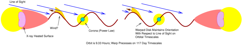
Figure 6.— A possible model for the behavior of V1408 Aql (not to scale). Optical modulation is due to partial eclipsing of a warped disk. Long term X-ray variations are due to the changing orientation of the warp. The X-ray power law is due to Comptonization within a corona. The $\sim 1$ keV plasma component is due to a wind or possibly due to a disk atmosphere.

Short Term X-ray Variability

Although we only have upper limits for the amplitude of the $10^{-3}$–$16$ Hz variability, these limits are consistent with the few observations of BHC and some NS-LMXB in nearly “pure” soft states (Miyamoto (1994)). For examples of BHC high/soft states, with little or no discernible hard tail wherein short term variability is presented, see Grebenev et al. (1991) for an observation of GX 339$-$4, Treves et al. (1988) for an observation of LMC X-3, Ebisawa, Mitsuda & Inoue (1989) for an observation of LMC X-1, and Miyamoto et al. (1994) for observations of Nova Muscae. The PSD presented in these works typically have a PSD level of $(\rm rms)^{2}/{\rm Hz}\approx 10^{-3}$ at 0.01 Hz, which decreases as $f^{-0.7}$ for higher Fourier frequencies and an rms variability of $\approx 3\%$ in the $10^{-2}$–$30$ Hz range. This is slightly below the upper limits presented in Figure 4.

The ‘normal branch’ of the NS-LMXB GX5+1 also has a similar amplitude and shape PSD as described above for high/soft state BHC; however, its energy spectrum consists of both a 1 keV MCD component and a 2 keV blackbody spectral component (Miyamoto (1994), and references therein). The high/soft state of Cir X-1 has been similarly modeled (Miyamoto (1994), and references therein). If V1408 Aql had weak 1–10 Hz variability comparable to that discussed by Miyamoto (1994) for Cir X-1, our observations would have detected it. Other soft neutron star sources with luminosities of ${\cal O}(10\%)$ Eddington (the approximate luminosity of V1408 Aql, if it were a 1.4 M_⊙ neutron star given our hypothesis of a highly inclined disk), especially the bright atoll sources such as GX13+1, GX3+1, GX9+1, and GX9+9, can also exhibit “very low frequency noise” with approximately 5% rms variability (Hasinger & van der Klis (1989)). The $10^{-4}$–100 s low amplitude variability in the light curves of these sources has been interpreted as intermittent, slow nuclear burning on the surface of the neutron star (Bildsten (1993, 1995)). Low frequency variability at such a level is absent in V1408 Aql. Furthermore, bright atoll sources often show a 0.1–10 Hz power spectrum in excess of the upper limits discussed here (Hasinger & van der Klis (1989)). The level of the 0.1–10 Hz PSD seen in GX13+1 (Homan et al. (1998)), for example, also would have been easily detected in the PSD of V1408 Aql, yet was not.

Black hole or neutron star?

The nature of the compact object as of now is not clear. The general picture outlined above is similar to that seen in neutron star X-ray binaries such as Sco X-1, Cyg X-2, and others. Yaqoob, Ebisawa & Mitsuda (1993) pointed out that the normalization of the best-fit MCD model appears to indicate that the compact object is a neutron star. This argument, however, strongly relies on the assumed distance to V1408 Aql, for which no compelling measurement exists (a lower limit of 2.5 kpc comes from the fact that the ASCA and ROSAT measured $N_{\rm H}$ values are consistent with the full galactic column), and also relies on the assumption that the accretion disk is seen closer to face on. The recent optical and soft X-ray variability measurements, however, make a large inclination more probable.

Taking these points into account and assuming for the sake of argument a source distance of 7 kpc, then the overall flux of V1408 Aql is comparable to that of the high state of the black hole candidate GX 339$-$4, which is a very plausible BHC. The upper limits to the high frequency variability discussed above are consistent with previously observed BHC power spectra in high/soft states. If transitions from the hard state to the soft state occur at 5%-10% of the Eddington luminosity (see Nowak (1995)), then the compact object in V1408 Aql is consistent with being a 2–3 ${\rm M}_{\odot}$ black hole. Thus, although there is no compelling evidence that V1408 Aql contains a black hole, there also is no compelling evidence that V1408 Aql is a neutron star.

Conclusions

X-ray spectroscopy and the study of both the long term and the short term variability of V1408 Aql make a system geometry as that depicted in Figure 6 seem likely. A low-mass main sequence star serves, via Roche Lobe overflow, as the donor for a compact object which is surrounded by a large accretion disk which in turn dominates the system at all wavelength ranges. The accretion disk is surrounded by an optically thin plasma, either in the form of an accretion disk wind or a stationary accretion disk photosphere, which emits the observed X-ray line radiation. A small hot corona directly surrounding the compact object produces the hard X-ray power-law. The whole accretion disk precesses on a time scale of about 117 d, obscuring the central region and causing the power-law tail to periodically disappear and reappear. Also on these long timescales, the changing view of the warp causes the orbital modulation of the optical light-curve (due to partial obscuration of the outer accretion disk) to vary from sinusoidal (Thorstensen (1987)) to a more complex pattern (Hakala, Muhli & Dubus (1999)).

The nature of the compact object in V1408 Aql is still ambiguous. We have put forth a hypothesis, however, that might explain the observed phenomenology and makes predictions that are observationally testable. X-ray monitoring over the 117 d period with an instrument like RXTE or BeppoSAX should reveal whether the X-ray power-law tail really does periodically disappear and reappear as predicted by our model. Furthermore, if the source is at 10% $L_{\rm Edd}$ and contains a neutron star, then about one “Type I” microburst per day might be expected (Bildsten (1995)). This should be easily observable during such a campaign. One might also hope to find “kilohertz QPO” (van der Klis (1998)), as are often associated with atoll sources. For these latter two possibilities, however, we note that some of the brighter atoll sources such as GX13+1 have yet to exhibit kilohertz QPO (Homan et al. (1998), and references therein), and rarely exhibit Type I bursts (see, for example, Matsuba et al. (1984), and references therein). Finally, high spectral resolution observations as will be provided by the upcoming new generation of X-ray instruments, such as the gratings on the Advanced X-ray Astronomy Facility (AXAF) and the X-ray Multiple Mirror Mission (XMM), will provide the spectral resolution necessary for resolving and studying the Fe L complex. This will allow the application of plasma spectroscopic diagnostics (e.g., Liedahl et al. (1992)) to the study of this fascinating source.

Appendix A Data Analysis Methodology

A.1. RXTE Data Analysis

Our RXTE data were analyzed using the same procedure as that for our analysis of the spectrum of GX 339$-$4 (Wilms et al. (1998a)). Screening criteria for the selection of good on-source data were that the source elevation was larger than 10^∘. Data measured within 30 minutes of passages of the South Atlantic Anomaly or during times of high particle background (as expressed by the “electron ratio” being greater than 0.1) were ignored. Using these selection criteria, a total exposure time of 27 ksec was obtained. To increase the signal to noise level of the data, we restricted the analysis to the first anode layer of the proportional counter units (PCUs) where most source photons are detected (the particle background is almost independent of the anode layer), and we combined the data from all five PCUs.

To take into account the calibration uncertainty of the PCA we applied the channel dependent systematic uncertainties described by Wilms et al. (1998a). These uncertainties were determined from a power-law fit to an observation of the Crab nebula and pulsar taking into account all anode chains; however, they do also provide a good estimate for the first anode layer only since most of the photons are detected in this layer.

Since V1408 Aql has a comparably small count rate we are able to use the new background model for the PCA that was made available by the RXTE Guest Observers Facility (GOF) in 1998 June. The quality of this model was checked by looking at high detector channels which are completely background dominated. Although the measured count rate of V1408 Aql was at the high end of the applicability of the new background model, the agreement between the model and the measured background was good. This is in part due to the fact that V1408 Aql is a very soft source which allows greater latitude in using the background model for faint sources. Remaining background residuals were minimized by using the XSPEC “corfile” facility which renormalizes the background flux to decrease the best fit $\chi^{2}_{\rm red}$. The corrections applied to the background flux were on the order of $\lesssim$1.5%, indicating that at least for this source the background model provides a good background estimate. Since the spectrum is completely background dominated above 20 keV, and due to the calibration uncertainty below 3 keV, we restricted the spectral analysis to the range from 3 to 20 keV.

For the timing analysis, we generated lightcurves from the ‘GoodXenon’ data. Note that although there are short data gaps of 1–4 s duration that are flagged by commensurate jumps in the value of the time coordinate from one data bin to the next, there are occasional data gaps where the extraction software generates a continuous series of time bins despite the data losses. These data gaps do not appear in lightcurves generated from the ‘standard2f’ data (which is processed by a different event analyzer on-board RXTE). These gaps can be recognized, however, in the high time resolution data by searching for any sequence, 1 s or greater in length, of time bins with zero count rate. Four such ‘unflagged’ sequences, with 16 s duration each, were found in our data. (Aside from these four 16 s sequences, there were a few instances where two $1/32$ s time bins in a row would have zero detected counts. The lack of counts in these bins were consistent with counting statistics, and we did not consider these to be data gaps.) The power spectra that we presented in Figure 4 were made from continous data segments without internal data gaps. If we include data segments with the unflagged data gaps in the calculation of the PSD, we obtain a low amplitude (5% rms) PSD that is flat from $10^{-3}$–$10^{-2}$ Hz and is exponentially cutoff at higher Fourier frequencies. In fact, the presence of unflagged data gaps can be deduced from such a characteristic PSD shape (Wijnands 1999, priv. comm.).

A.2. ASCA Data Analysis

We extracted data from the two solid state detectors (SIS0, SIS1) and the two gas detectors (GIS2, GIS3) onboard ASCA by using the standard ftools as described in the ASCA Data Reduction Guide (Day et al. (1998)). The data extraction regions were limited by the fact that all the observations were in 1-CCD mode and that the source was placed close to the chip edge. To maximize the extraction regions, we chose rectangular regions of $6^{\prime}\times 8^{\prime}$ and $6^{\prime}\times 7^{\prime}$ for SIS0 and SIS1, respectively. Choosing a rectangular region does not effect the shape of the extracted spectrum; however, the ASCAARF ancillary response matrix generator assumes a circular region, so the flux normalization is slightly off (hence the $\approx 30\%$ normalization differences between the SIS and GIS detectors in Table 2). For the GIS detectors we chose circular regions centered on the source each with a radius of $13^{\prime}$.

The SIS count rate for V1408 Aql is large enough that the central regions of the CCD suffer from pileup (i.e., two or more events being registered as a single event). Estimates of the amount of this pileup can be found in the appendix presented by Ebisawa et al. (1996). Based upon our measured spectrum and these estimates, we chose to exclude from analysis central rectangular regions with dimensions of $4^{\prime}\times 3^{\prime}$ and $3^{\prime}\times 3^{\prime}$ for SIS0 and SIS1, respectively. With these exclusions, we estimate that pileup will contribute less than 1% of the counts at 10 keV.

We used the SISCLEAN and GISCLEAN tools (Day et al. (1998)), with the default values, to remove hot and flickering pixels. As the spectrum of V1408 Aql is very similar to the low flux level of Cir X-1 described by Brandt et al. (1996), we filtered the data with the same cleaning criteria outlined in that work; however, we took the slightly larger values of $10^{\circ}$ for the minimum elevation angle and 7 $\mbox{GeV}/c$ for the rigidity. Also similar to the work of Brandt et al. (1996), we formed background estimates by extracting a circular region of radius $5^{\prime}$ near the edge of the detector for the GIS observations. For the SIS observations, we chose L shaped regions near the corner of the chip opposite from the source. Background, however, contributes relatively little to the observations.

We rebinned the spectral files so that each energy bin contained a minimum of 20 photons. We retained SIS data in the 0.6 to 10 keV range and GIS data in the 1 to 10 keV range. The cross-calibration uncertainties among the instruments were accounted for by introducing a multiplicative constant for each detector in all of our fits. As discussed above, the resulting data files showed reasonable agreement between all four detectors.

A.3. ROSAT Data Analysis

The extraction of the ROSAT spectrum was performed using the standard ROSAT PSPC data analysis package Extended X-ray Scientific Analysis System (EXSAS) (Zimmermann et al. (1998)) following the procedures described by Brunner et al. (1997). Source counts were extracted from a circular region centered on the position of V1408 Aql with a radius of $2^{\prime}$, while the background was extracted from an annulus centered on the source from which source counts from detected background sources were removed. A correction for the telescope vignetting was applied to the standard ROSAT response matrix. The spectrum was then rebinned into 26 channels of $\sim 10000$ counts each to ensure an even signal to noise ratio over the whole ROSAT energy band. As for RXTE and ASCA, the spectral analysis of the extracted data was then performed with XSPEC, ignoring data measured below 0.5 keV and above 2.5 keV.

References

- Arnaud (1996) Arnaud, K. A., 1996, in Astronomical Data Analysis Software and Systems V, ed. J. H. Jacoby, J. Barnes, (San Francisco), 17
- Balbus & Hawley (1991) Balbus, S.A., & Hawley, J.F. 1991, ApJ, 376, 214
- Belloni & Hasinger (1990) Belloni, T., & Hasinger, G., 1990, A&A, 230, 230
- Bildsten (1993) Bildsten, L., 1993, ApJ, 418, L21
- Bildsten (1995) Bildsten, L., 1995, ApJ, 438, 852
- Brandt et al. (1996) Brandt, W. N., Fabian, A. C., Dotani, T., Nagase, F., Inoue, H., Kotani, T., & Segawa, Y., 1996, 283, 1071
- Brunner et al. (1997) Brunner, H., Müller, C., Friedrich, P., Dörrer, T., Staubert, R., & Riffert, H., 1997, A&A, 326, 885
- Cowley, Hutchings & Crampton (1988) Cowley, A. P., Hutchings, J. B., & Crampton, D., 1988, ApJ, 333, 906
- Cowley et al. (1991) Cowley, A. P., et al., 1991, ApJ, 381, 526
- Davies (1990) Davies, S. R., 1990, MNRAS, 244, 93
- Day et al. (1998) Day, C., Arnaud, K., Ebisawa, K., Gotthelf, E., Ingham, J., Mukai, K., & White, N., 1998, The ASCA Data Reduction Guide, Technical report, (Greenbelt, Md.: NASA Goddard Space Flight Center), Version 2.0
- Dickey & Lockman (1990) Dickey, J. M., & Lockman, F. J., 1990, ARA&A, 28, 215
- Dove et al. (1997) Dove, J. B., Wilms, J., Maisack, M. G., & Begelman, M. C., 1997, ApJ, 487, 759
- Ebisawa, Mitsuda & Inoue (1989) Ebisawa, K., Mitsuda, K., & Inoue, H., 1989, PASJ, 41, 519
- Ebisawa et al. (1996) Ebisawa, K., Ueda, Y., Inoue, H., Tanaka, Y., & White, N. E., 1996, ApJ, 467, 419
- Esin, McClintock & Narayan (1997) Esin, A. A., McClintock, J. E., & Narayan, R., 1997, ApJ, 489, 865
- Giacconi et al. (1974) Giacconi, R., Murray, S., Gursky, H., Kellogg, E., Schreier, E., Matilsky, T., Koch, D., & Tananbaum, H., 1974, ApJS, 27, 37
- Grebenev et al. (1991) Grebenev, S. A., Syunyaev, R., Pavlinsky, M. N., & Dekhanov, I. A., 1991, Sov. Astron. Lett., 17, 413
- Hakala, Muhli & Dubus (1999) Hakala, P. J., Muhli, P., & Dubus, G., 1999, MNRAS, submitted
- Hasinger & van der Klis (1989) Hasinger, G., & van der Klis, M., 1989, A&A, 225, 79
- Homan et al. (1998) Homan, J., Klis, M. v., Wijnands, R., Vaughan, B., & Kuulkers, E.,
- Horne & Baliunas (1986) Horne, J. H., & Baliunas, S. L., 1986, ApJ, 302, 757
- Kallman et al. (1996) Kallman, T. R., Liedahl, D., Osterheld, A., Goldstein, W., & Kahn, S., 1996, ApJ, 465, 994
- Kallman, Vrtilek & Kahn (1989) Kallman, T. R., Vrtilek, S. D., & Kahn, S. M., 1989, ApJ, 345, 498
- Kemp et al. (1983) Kemp, J. C., et al., 1983, ApJ, 271, L65
- Larwood (1998) Larwood, J., 1998, MNRAS, 299, L32
- Leahy et al. (1983) Leahy, D. A., Darbro, W., Elsner, R. F., Weisskopf, M. C., Sutherland, P. G., Kahn, S., & Grindlay, J., 1983, ApJ, 266, 160
- Levine et al. (1996) Levine, A. M., Bradt, H., Cui, W., Jernigan, J. G., Morgan, E. H., Remillard, R., Shirey, R. E., & Smith, D. A., 1996, ApJ, 469, L33
- Liedahl et al. (1992) Liedahl, D. A., Kahn, S. M., Osterheld, A. L., & Goldstein, W. H., 1992, ApJ, 391, 306
- Lochner & Remillard (1997) Lochner, J., & Remillard, R., 1997, ASM Data Products Guide, Version Dated August 27, 1997, http://heasarc.gsfc.nasa.gov/docs/xte/asm_products_guide.html
- Lomb (1976) Lomb, N. R., 1976, Ap&SS, 39, 447
- Maloney, Begelman & Nowak (1998) Maloney, P. R., Begelman, M., & Nowak, M. A., 1998, ApJ, in press
- Maloney & Begelman (1997) Maloney, P. R., & Begelman, M. C., 1997, ApJ, 491, L43
- Maloney, Begelman & Pringle (1996) Maloney, P. R., Begelman, M. C., & Pringle, J. E., 1996, ApJ, 472, 582
- Margon, Thornstensen & Bowyer (1978) Margon, B., Thornstensen, J. R., & Bowyer, S., 1978, ApJ, 221, 907
- Matsuba et al. (1984) Matsuba, E., Dotani, T., Mitsuda, K., Asai, K., Lewin, W.H.G., van Paradijs, J., & van der Klis, M., 1995, PASJ, 47, 575
- Mitsuda et al. (1984) Mitsuda, K., et al., 1984, PASJ, 36, 741
- Miyamoto (1994) Miyamoto, S., 1994, Time-variation from X-ray stars, Technical Report RN 548, (Tokyo: ISAS)
- Miyamoto et al. (1991) Miyamoto, S., Kimura, K., Kitamoto, S., Dotani, T., & Ebisawa, K., 1991, ApJ, 383, 784
- Miyamoto et al. (1994) Miyamoto, S., Kitamoto, S., Iga, S., Hayashida, K., & Terada, K., 1994, ApJ, 435, 398
- Miyamoto et al. (1992) Miyamoto, S., Kitamoto, S., Iga, S., Negoro, H., & Terada, K., 1992, ApJ, 391, L21
- Morgan et al. (1997) Morgan, E.H., Remillard, R.A., & Greiner, J., 1997, ApJ, 482, 993
- Nagase et al. (1994) Nagase, F., Zylstra, G., Sonobe, T., Kotani, T., Inoue, H., & Woo, J., 1994, ApJ, 436, L1
- Nowak (1995) Nowak, M. A., 1995, PASP, 107, 1207
- Nowak et al. (1999a) Nowak, M. A., Vaughan, B. A., Wilms, J., Dove, J., & Begelman, M. C., 1999a, ApJ, 510 in press
- Nowak et al. (1999b) Nowak, M. A., Wilms, J., & Dove, J. B., 1999b, ApJ, 517, in press
- Nowak et al. (1999c) Nowak, M. A., Wilms, J., Vaughan, B. A., Dove, J. B., & Begelman, M. C., 1999c, ApJ, 515, in press
- Priedhorsky & Terrell (1984) Priedhorsky, W. C., & Terrell, J., 1984, ApJ, 280, 661
- Priedhorsky, Terrell & Holt (1983) Priedhorsky, W. C., Terrell, J., & Holt, S. S., 1983, ApJ, 270, 233
- Pringle (1996) Pringle, J. E., 1996, MNRAS, 281, 357
- Raymond & Smith (1977) Raymond, J. C., & Smith, B. W., 1977, ApJS, 35, 419
- Remillard & Levine (1997) Remillard, R. A., & Levine, A. M., 1997, in All-Sky X-Ray Observations in the Next Decade, ed. N. Matsuoka, N. Kawai, (Tokyo: Riken), 29
- Ricci et al. (1996) Ricci, D., Asai, K., Israel, G. L., Mereghetti, S., Mitsuda, K., Parmar, A. N., & Stella, L., 1996, Mem. Soc. Astron. Ital., 67, 1039
- Ricci, Israel & Stella (1995) Ricci, D., Israel, G. L., & Stella, L., 1995, A&A, 299, 731
- Ross & Fabian (1993) Ross, R. R., & Fabian, A. C., 1993, 261, 74
- Scargle (1982) Scargle, J. D., 1982, ApJ, 263, 835
- Schandl (1996) Schandl, S., 1996, A&A, 307, 95
- Schulz, Hasinger & Trümper (1989) Schulz, N. S., Hasinger, G., & Trümper, J., 1989, A&A, 225, 48
- Schwarzenberg-Czerny (1989) Schwarzenberg-Czerny, A., 1989, MNRAS, 241, 153
- Shahbaz et al. (1996) Shahbaz, T., Smale, A. P., Naylor, T., Charles, P. A., van Paradijs, J., Hassall, B. J. M., & Callanan, P., 1996, MNRAS, 282, 1437
- Shakura & Sunyaev (1973) Shakura, N. I., & Sunyaev, R., 1973, A&A, 24, 337
- Singh, Apparao & Kraft (1994) Singh, K. P., Apparao, K. M. V., & Kraft, R. P., 1994, ApJ, 421, 753
- Smith, Beall & Swain (1990) Smith, H. A., Beall, J. H., & Swain, M. R., 1990, AJ, 99, 273
- Stark et al. (1992) Stark, A. A., Gammie, C. F., Wilson, R. W., Bally, J., Linke, R. A., Heiles, C., & Hurwitz, M., 1992, ApJS, 79, 77
- Stelzer et al. (1999) Stelzer, B., Wilms, J., Staubert, R., Gruber, D., & Rothschild, R., 1999, A&A, in press
- Tanaka & Lewin (1995) Tanaka, Y., & Lewin, W. H. G., 1995, in X-Ray Binaries, ed. W. H. G. Lewin, J. van Paradijs, E. P. J. van den Heuvel, (Cambridge), Chapt. 3, 126
- Thorstensen (1987) Thorstensen, J. R., 1987, ApJ, 312, 739
- Titarchuk (1994) Titarchuk, L., 1994, ApJ, 434, 570
- Treves et al. (1988) Treves, A., Belloni, T., Chiapetti, L., Maraschi, L., Stella, L., Tanzi, E. G., & van der Klis, M., 1988, ApJ, 325, 119
- van der Klis (1989) van der Klis, M., 1989, in Timing Neutron Stars, ed. H. Ögelman, E. P. J. van den Heuvel, (Dordrecht: Kluwer), 27
- van der Klis (1998) van der Klis, M., 1998, in Proc. Third William Fairbank Meeting, in press (astro-ph/9812395)
- Vaughan & Nowak (1997) Vaughan, B. A., & Nowak, M. A., 1997, ApJ, 474, L43
- Vrtilek et al. (1986) Vrtilek, S. D., Kahn, S. M., Grindlay, J. E., Seward, F. D., & Helfand, D. J., 1986, ApJ, 307, 698
- White & Marshall (1984) White, N. E., & Marshall, F. E., 1984, apj, 281, 354
- Wilms et al. (1998a) Wilms, J., Nowak, M. A., Dove, J. B., Fender, R. P., & di Matteo, T., 1998a, ApJ, submitted
- Wilms et al. (1998b) Wilms, J., Nowak, M. A., Dove, J. B., Pottschmidt, K., Heindl, W. A., Begelman, M. C., & Staubert, R., 1998b, in Highlights in X-ray Astronomy, ed. B. Aschenbach, M. Freyberg, in press
- Wilms et al. (1999) Wilms, J., Nowak, M. A., Pottschmidt, K., Heindl, W. A., & Begelman, M. C., 1999, ApJ, in preparation
- Yaqoob, Ebisawa & Mitsuda (1993) Yaqoob, T., Ebisawa, K., & Mitsuda, K., 1993, MNRAS, 264, 411
- Zhang & Jahoda (1996) Zhang, W., & Jahoda, K., 1996, Deadtime Effects in the PCA, Technical report, (Greenbelt: NASA GSFC)
- Zhang et al. (1995) Zhang, W., Jahoda, K., Swank, J. H., Morgan, E. H., & Giles, A. B., 1995, ApJ, 449, 930
- Zimmermann et al. (1998) Zimmermann, U., Boese, G., Becker, W., Belloni, T., Döbereiner, S., Izzo, C., Kahabka, P., & Schwentker, O., 1998, EXSAS User’s Guide, 5th edition, Technical report, (Garching: Max-Planck-Institut für Extraterrestrische Physik)