Values of H₀ from Models of the Gravitational Lens $0957+561$

Abstract

The lensed double QSO 0957+561 has a well-measured time delay and hence is useful for a global determination of H₀. Uncertainty in the mass distribution of the lens is the largest source of uncertainty in the derived H₀. We investigate the range of H₀ produced by a set of lens models intended to mimic the full range of astrophysically plausible mass distributions, using as constraints the numerous multiply-imaged sources which have been detected. We obtain the first adequate fit to all the observations, but only if we include effects from the galaxy cluster beyond a constant local magnification and shear. Both the lens galaxy and the surrounding cluster must depart from circular symmetry as well.

Lens models which are consistent with observations to 95% CL indicate $H_{0}=104^{+31}_{-23}(1-{\bar{\kappa}_{30^{\prime\prime}}})$ ${\rm km}\,{\rm s}^{-1}\,{\rm Mpc}^{-1}$. Previous weak lensing measurements constrain the mean mass density within 30″ of G1 to be ${\bar{\kappa}_{30^{\prime\prime}}}=0.26\pm 0.16$ (95% CL), implying $H_{0}=77^{+29}_{-24}$ ${\rm km}\,{\rm s}^{-1}\,{\rm Mpc}^{-1}$ (95% CL). The best-fitting models span the range 65–80 ${\rm km}\,{\rm s}^{-1}\,{\rm Mpc}^{-1}$. Further observations will shrink the confidence interval for both the mass model and ${\bar{\kappa}_{30^{\prime\prime}}}$.

The range of H₀ allowed by the full gamut of our lens models is substantially larger than that implied by limiting consideration to simple power law density profiles. We therefore caution against use of simple isothermal or power-law mass models in the derivation of H₀ from other time-delay systems. High-S/N imaging of multiple or extended lensed features will greatly reduce the H₀ uncertainties when fitting complex models to time-delay lenses.

1 Motivations

The accurate measure of the time delay between the two images of the gravitationally lensed quasar Q0957+561 (Kundić et al. 1996) leads, in principle, to a measure of H₀ accurate to a few percent (Refsdal 1964). This accuracy in H₀ is achievable only when the gravitational potential $\phi$ of the lens (or, equivalently, its surface mass distribution $\Sigma$) is also determined to an accuracy of a few percent. At present, uncertainties in the lens model dominate the uncertainty in H₀. The goal of this paper is to determine which, if any, models for the lens are consistent with the many observational constraints on this system, and to thence find the range of H₀ values implied by the family of acceptable lens models.

A number of authors have investigated mass models for $0957+561$ over the 20 years since its discovery. Gorenstein, Falco, & Shapiro (1988a; followed by Falco, Gorenstein, & Shapiro 1991, hereafter FGS) pointed out that any lens model constrained by the positions or magnifications of lensed objects are subject to a “mass sheet degeneracy.” If a mass distribution $\Sigma(\vec{x})$ successfully reproduces the lensing behavior, then an altered model with mass distribution $(1-\kappa)\Sigma(\vec{x})+\kappa\Sigma_{\rm crit}$ will have identical optical characteristics yet yield a value for H₀ differing by a factor $1-\kappa$. Since the primary lensing galaxy G1 is the brightest member of a modest galaxy cluster, we fully expect there to be a dark matter component which is slowly varying across the region of multiple imaging. The lens modeling process can hence be broken into two fairly distinct problems: first, we must determine a “strong lensing model” which prescribes a mass distribution $\Sigma_{0}$, over the central $\approx 10\arcsec$ region, that accurately reproduces the observed strongly distorted or multiply imaged sources in this area. Second, we must find a way to measure the average mass density across the strong-lensing area or otherwise find the proper $1-\kappa$ scaling for $\Sigma_{0}$ (and hence H₀).

The primary focus of this paper is to investigate several broad classes of candidate mass distributions for the G1-cluster system, and find what range of H₀ is produced by those which satisfy the observational constraints on the lens. In §2 we delineate these constraints, which are now more extensive than available to Grogin & Narayan (1996, hereafter GN). In §3 we describe the parametric models of the mass distribution which we will use to fit the strong-lensing constraints, and the a priori constraints we impose on these models in order to keep them “astrophysically reasonable.” In §4 we present the results of the fits, including the best-fit models and the range of H₀ allowed before application of the $1-\kappa$ correction. §2–4 are somewhat involved, and many readers may wish to skip through to the end of §4 for a summary of the model-fitting results. In §5.1 we use the weak-lensing measurements of Fischer et al. (1996, hereafter Paper I) to resolve the mass-sheet degeneracy. In §6 we discuss the possibilities for improvement in the constraints on H₀ that we derive. In §7 we conclude.

2 Strong-Lensing Constraints

The $0957+561$ system has been observed in detail at wavelengths from radio to x-ray, and displays a rich variety of lensed features. We discuss here the numerical constraints that these observations place upon models of the lens optics. Table 1 summarizes the constraints we have adopted for our modeling.

Table 1: Adopted Constraints on Lens Models

Object	$x$	$y$	Flux Ratio
Quasar A	$+1.408(0)$	$+5.034(0)$	$f_{QB}/f_{QA}=0.74(2)$
Quasar B	$+0.182(0)$	$-1.018(0)$
Jet A5	$+0.0164(5)$	$+0.0457(5)$	$f_{B5}/f_{A5}=0.63(3)$
Jet B5	$+0.0181(5)$	$+0.0559(5)$
Knot 1	$+0.06(5)$	$-2.55(5)$	$\ln(f_{K2}/f_{K1})=0.0(7)$
Knot 2	$+0.48(5)$	$-2.43(5)$
Blob 2	$-1.54(5)$	$-0.05(5)$	$\ln(f_{B3}/f_{B2})=0.9(3)$
Blob 3	$+2.86(5)$	$+3.47(5)$

Note. — Image positions and flux ratios for all 4 pairs of multiple images are given, with 1-sigma uncertainties in parentheses. All sources assumed at $z=1.41$ and lens assumed at $z=0.356$. See §2 for details and references.

2.1 Quasar and G1 Positions: 2 constraints

The positions of the A and B quasar cores are determined to micro-arcsecond accuracy by the VLBI measurements of Gorenstein et al. (1988b). We will adopt their positions and consider them to be known exactly. The requirement of a common source position for the A and B quasar images places two (exact) constraints on the lens model. In our modeling procedure, these are solved by adjusting the two components of external shear (see §4.1).

The WFPC2 observations of Bernstein et al. (1997, hereafter Paper II) showed that the optical quasar separation agrees with the VLBI separation to the measurement precision of a few milli-arcseconds. Paper II also shows that the optical peak and centroid of G1 coincide with the VLBI point source G^′ (Gorenstein et al. 1988b) to within 10 mas. We will therefore adopt the VLBI position of G^′ as the center of G1, and consider its 1 mas uncertainty to be negligible. We adopt the G^′ position as the center of our mass distributions, so the G1 center does not appear as an adjustable parameter in our models.

We will henceforth measure all object positions in a coordinate system centered on G^′, with $x$ axis pointing West and $y$ axis North (J2000), with units of arcseconds unless otherwise specified. Position angles will be measured counter-clockwise from the $x$-axis, 90° different from the astronomical North-through-East convention.

2.2 Quasar Jets: 2 Constraints

The most detailed images to date of the VLBI jets extending from the A and B quasars are given by Garrett et al. (1994), and are re-analyzed by Barkana et al. (1998, hereafter BLFGKS). Both authors fit to each jet a model containing a core and five additional Gaussian jet components (A2–A6, B2–B6). A proper lens model should map each of these 5 pairs of objects to common sources. Each of these papers derives a local transformation which maps the A jet positions and fluxes into their B counterparts. To simultaneously fit the positional constraints and the flux magnification constraints (see the next section), it is necessary to allow this map to be more complex than a linear transformation. Both papers fit a model in which the relative magnification matrix is allowed to vary in a limited fashion along the jet (e.g. the magnification eigenvectors are fixed but the eigenvalues vary along the jet). We have, therefore, two choices in implementing the jet constraints in our models. We can either fit to some or all of the jet positions and fluxes directly, or we can fit by trying to match the 6 derived parameters that describe the local behavior of the relative magnification matrix. We choose the former method for two reasons. First, computing the gradient of the local magnification matrix would require computing complicated ratios of third derivatives of the model potential, which would slow our numerical methods substantially. Second, to reduce the behavior of the local magnification matrix to 6 parameters, Garret et al. and BLFGKS assume that the eigenvectors of the magnification do not vary with position. This may not be the case for our model lenses, and it is not clear how, in this case, we should implement a fit to the parameters of a fixed-eigenvector model.

Fitting directly to the jet component positions could add 10 constraints to our model, but in fact most of this information is redundant for any realistic model (flux ratio constraints are discussed below). The jet components lie nearly along a line, and their positions are consistent with a constant relative magnification matrix between the A and B images. The nearly-linear arrangement of the sources further means that only two components of the relative magnification matrix are well constrained. We can therefore extract nearly all the useful information from the jet components by considering only the brightest and best-measured pair, A5 and B5. We will use the positions from the “partial fit” of BLFGKS (their Table 2), for which in fact all the jet positions are forced to map smoothly from A to B.

The positions of components A5 and B5 are determined to high precision, with formal uncertainties of only $\approx 0.1$ mas, or 0.2% of their displacements from the quasar cores. For the reasons outlined in Appendix A, we believe that the use of such small uncertainties may be unjustified and/or could constrain the $\chi^{2}$ minimum to a misleadingly narrow region of parameter space. When fitting models, we give the models more freedom by widening the error ellipse for each jet component to be a circle with radius equal to 1% of the jet’s displacement from the quasar cores. In actuality we find that the models do not require this additional freedom: retaining the original BLFGKS error estimates changes the minimum $\chi^{2}$ by $<0.1$ and changes the H₀ bounds by $<1\%$.

2.3 Quasar/Jet Flux Ratios: 2 Constraints

Determination of the flux ratios between the A and B images is confounded by three effects: first, small sources can vary on time scales comparable to the 1.1-year time delay. Second, the quasar continuum source is likely small enough to be microlensed by stars in G1, which can cause decades-long perturbations to the flux ratio. Third, Connor et al. (1992) argue that the flux ratio varies significantly along the jet, as the core is closer to the lensing caustic than the jets.

Garrett et al. (1994) summarize the various constraints on flux ratios. The components of the jet should be large enough to be free of microlensing and temporal variation problems. Their measured flux ratio for B5/A5 combined with the previous independent VLBI jet flux ratio measurements give a flux ratio of $0.63\pm 0.03$ at the position of jet component 5. We also know (from the jet images) that there must be a parity flip between images A and B.

Measuring the flux ratio at the core is more difficult because microlensing and time variation are likely. Garrett et al. (1994) cite several attempts to measure the core flux ratio in the radio by interpolating observations at different epochs and/or frequencies to make up for the 1.1-year time delay. All of these, however, are imprecise or used a time delay value now excluded by the data. Schild & Smith (1991) measured broad-line Mg 2 fluxes from the two quasars at two epochs 1.1 years apart. The line flux originates from a region believed large enough to be unaffected by microlensing, and the two epochs serve to remove any source variability. They report a flux ratio of $0.75\pm 0.02$. Spectrophotometric observations such as this are subject to many systematic difficulties, and the quoted errors encompass only counting statistics, so we will be conservative and double the quoted uncertainty on this value.

More recently Haarsma et al. (1999) estimate a core flux ratio from a long VLA time series. The VLA does not resolve the core from the jets, but if one presumes that the jets are invariant on decade time scales, then the ratio of fluctuations in the A and B fluxes (when phased by the time delay), gives a magnification ratio for the (varying) core flux only. The core radio continuum source is believed to be large enough to avoid microlensing amplification. Analyses of different frequencies and subsets of the data yield flux ratios from 0.72 to 0.76; we will therefore adopt $0.74\pm 0.02$ as the core flux ratio, which is consistent with all optical and VLA measurements.

Most recently BLFGKS derive core and Jet 5 flux ratios of $0.74\pm 0.06$ and $0.64\pm 0.03$, respectively, from their “partial fit” to the positions and fluxes of the VLBI jets. This is comfortingly consistent with the values we have adopted from other sources (though the data upon which the jet flux ratio is based is the same as the Garrett et al. data).

2.4 Arc System: 6 Constraints

Paper II gives the positions and fluxes of a number of faint objects discovered in the strong-lensing region in WFPC2 images. Three resolved objects, “Blob 2,” “Blob3,” and an apparent arc, are close enough to G1 to expect that they are multiply imaged. The arc contains two bright spots, a pattern which suggest that these “Knots” sit astride the critical line and are multiple images of a bright spot in the source. We adopt the positions and uncertainties of Knots 1 and 2 given in Paper II. In addition, we demand that Knots 1 and 2 have opposite parities, and that their flux ratio be $\ln(f_{K1}/f_{K2})=0\pm 0.7$, in accord with the (poorly) determined magnitudes from Paper II. This adds 3 constraints to the model. We also enforce the qualitative constraint that a model must “fold” the source of the arc back over on itself, i.e. we expect that the arc is a greatly magnified image of a small source, rather than an image of some intrinsically very elongated source. In practice this qualitative constraint forces the G1 matter distribution to have a position angle (PA) roughly aligned with the visible galaxy rather than perpendicular to it (see §4). This conclusion is in line with that of Keeton, Kochanek, & Falco (1998), who find that the application of isothermal ellipsoid mass models to 17 well-measured lens systems yeilds a position angle within $\approx 10\arcdeg$ of the visible $PA$ in nearly all cases.

Any reasonable model for the lens shows that the sources of Blobs 2 and 3 could be quite close to each other. It is also clear that if either source is at a redshift $z\gtrsim 0.5$, then a counterimage should be visible. The only candidate counterimage for Blob 2 is Blob 3, and vice-versa, so there seems to be little risk in assuming these two objects to be images of the same source. We adopt this constraint in our models, using the positions and uncertainties from Paper II. We also constrain the flux ratio of Blob 2 to Blob 3 to be $\ln(f_{B2}/f_{B3})=-0.9\pm 0.3$. This implies a $1.0\pm 0.3$ mag difference between the Blobs, which differs a bit from the $1.3\pm 0.14$ mag difference in Table 2 of Paper II. We have revised our estimate of the magnitude of Blob 3 by 0.3 mag. The revision reflects a changed estimate of the local sky value, which is difficult to evaluate due to residual flux from the quasar and G1 images.

The magnification ratio will change rapidly across the extent of the blobs, so their observed flux ratio is actually an integral of the magnification ratio across the extent of the source. Such a calculation is impractical for our models (the shape of the source is not well known anyway), so our constraint is only upon the magnification ratio at the object centroids. For this reason the uncertainty on the magnification ratio used to constrain the model is higher (0.3 mag) than the stated measurement uncertainties on the relative flux (0.14 mag). With improved S/N on the images of the Blobs it should be possible to produce more specific constraints (and better object names).

The two multiply-imaged systems provide 3 constraints each (2 position, 1 flux) to the model. There are, however, two additional degrees of freedom which are introduced, namely the redshifts of the arc and blob source objects. If we leave these source redshifts as free parameters in the model fits described below, we find the best fits have the arc and blob sources both very close to the quasar in redshift. Avruch et al. (1997) obtain the same result, though BLFGKS differ. Furthermore, the arc and blob sources are separated by only a few tenths of an arcsecond in the source plane in these models. This strongly suggests that (a) the arc is a highly magnified double image of an extension of the blob source that crosses a caustic, and hence the arc and blob have common redshift; (b) the arc/blob source object is at the quasar redshift. The a priori most likely distance for the arc and blob sources is of course near the quasar, since quasars are found in large galaxies and since galaxies are clustered in space.

More evidence that the arc and blob sources are at the quasar redshift is given by a recent HST/NICMOS $H$-band image of this system (Kochanek et al. 1998), which shows a spectacular pair of arcs surrounding each quasar image, presumably the images of the quasar host galaxy. The WFPC2 $V$-band Blobs 2 and 3 and arc all lie within the envelope of the NICMOS arcs. It thus seems extremely likely that the Blob and WFPC2 arc sources are “hot spots,” bright in rest-frame UV, within or associated with the quasar host galaxy. We will therefore assume a common redshift for all these sources.

2.5 Other Information

2.5.1 Arcs

Among the many interesting features revealed in the wealth of imaging of the $0957+561$ system are extended arc-like structures seen in NICMOS near-IR images (Kochanek et al. 1998), in high-S/N radio imaging (Harvanek et al. 1997; Porcas et al. 1996, Avruch et al. 1997), and perhaps even in x-ray images (Jones et al. 1993, Chartas et al. 1995); It is difficult to incorporate this information into our lens models unless the images have sufficiently high S/N and resolution that one can identify a correspondence between multiply imaged features in the surface-brightness maps. The x-ray “arcs” are a marginal detection and not yet useful as lens model constraints.

Avruch et al. (1997) demonstrate that the VLA arc can be adequately reproduced by judicious placement of sources. Other features of the VLA and Merlin maps are similar in that they can be reproduced qualitatively by proper source placement in all our models, so they do not add information to our current modeling. Ongoing improvements in the radio maps, coupled with some type of CLEAN or maximum entropy reconstruction algorithm for lenses (e.g. Wallington et al. 1996, Ellithorpe et al. 1996) or other software for modeling diffuse sources, will certainly be of use in testing and limiting the lens models.

The NICMOS images are, at this writing, preliminary and may perhaps yield quite useful constraints if sufficient S/N can be achieved. Kochanek et al. (1998) state that the direction of extension of the A and B arcs are sufficient to rule out the GN model.

2.5.2 VLA Jets

VLA images of the system (Greenfield et al. 1985) show extended jets (labelled C, D, and E) extending several arcseconds from the A quasar. The absence of jet images about the B quasar could be used as a model constraint. In all of our models, the source regions for the C, D, and E jets are either singly imaged, or perhaps have highly demagnified images leading from B toward the center of G1. Avruch et al. (1997) may have detected a counterimage of a low-surface-brightness extension of the E jet, but the resolution is as yet too poor to yield much information.

2.5.3 No Quasar C

The failure to detect a third quasar image is not a useful constraint on our models. As noted in Paper II, the stellar light density of G1 continues a power-law increase toward the center, as do all other observed elliptical galaxies (Gebhardt et al. 1996). For surface-density power laws with exponents near the isothermal value of $-1$, the third image will be absent or highly demagnified. The third image is also easily “captured” by a star and further demagnified. The properties of the third image might constrain the mass distribution in the central 0$\farcs$1 of G1, but this mass has little effect on H₀.

2.5.4 G1 Velocity Dispersion

High-accuracy measurements of the stellar velocity dispersion of G1 are presented by Tonry & Franx (1998; see also Falco et al. 1997). While the velocity dispersion of G1 may be used to break the mass-sheet degeneracy (§5.1), we mention here a different use. Over a range of $\pm 3\arcsec$ from the center of G1, Tonry & Franx detect a change of $\lesssim 10\%$ in the velocity dispersion. Given their good seeing (0$\farcs$7) and the sharp central cusp in the G1 luminosity profile (Paper II), this measurement shows that the velocity dispersion of G1 is nearly constant over a range 1″–3″ in projected radius. Thus the radial mass profile of G1 is nearly isothermal, $\alpha=-1$ in the notation of Equation (12) below. A full consideration of the constraints imposed by this measurement is beyond the scope of this paper—see Romanowsky & Kochanek (1998) for the significant steps toward constraining the G1 mass with stellar velocity data. We will, however, assume the very crude and conservative constraint that the power-law index of the projected G1 mass density at $\approx 1\arcsec$ radius satisfies $-1.5\leq\alpha\leq-0.5$. In a naive interpretation (i.e. spherically symmetric galaxy with isotropic velocities), a mass index at these upper or lower limits would lead to a 30% rise or fall (100 km s^-1) in velocity dispersion in the data of Tonry & Franx, which can clearly be excluded.

2.5.5 Cluster Location

The weak lensing mass map in Paper I shows the peak of the cluster mass distribution located to the northeast of G1. This displacement is only marginally significant ($\approx 1.5\sigma$); one cannot from this data alone exclude the possibility that the cluster is centered on G1. Paper I also shows that the light distribution of the cluster galaxies is peaked to the NE of G1, though again not at high significance. In what follows we will find further evidence from the strong-lensing models that the cluster mass peaks in the NE or SW quadrant. We believe that the concurrence of these three weak, but independent, lines of evidence is sufficient to apply a constraint that the cluster mass density be increasing to the NE quadrant of G1.

3 Mass Models

3.1 Terminology

We define in the usual fashion the dimensionless 2d gravitational potential $\phi(\vec{x})$ via

$$\nabla^{2}\phi(\vec{x})=2\kappa(\vec{x})=2\Sigma(\vec{x})/\Sigma_{\rm crit},$$ (1)

where the critical density $\Sigma_{\rm crit}$ is determined by the angular diameter distances $D_{OL}$, $D_{LS}$, $D_{OS}$ between observer, lens, and source:

$$\Sigma_{\rm crit}={{4\pi c^{2}}\over G}{{D_{OS}}\over D_{OL}D_{LS}}.$$ (2)

For our application the redshift of the observer is zero, of the lens is $z_{L}=0.356$ (Tonry & Franx 1998), and of the sources $z_{S}=1.41$ (Weymann et al. 1979). The position $(u,v)$ in the source plane of an object viewed at $(x,y)$ in the image plane is

$$\begin{array}[]{lcr}u&=&x-\phi_{,x}\\ v&=&y-\phi_{,y}\end{array}.$$ (3)

Subscripts after the comma denote differentiation with respect to the given coordinate(s). The inverse of the magnification matrix in this region is

$$\bf M^{-1}=\left(\begin{array}[]{cc}1-\phi_{,xx}&-\phi_{,xy}\\ -\phi_{,xy}&1-\phi_{,yy}\\ \end{array}\right)$$ (4)

The time delay between two images at $\vec{x}_{A}$ and $\vec{x}_{B}$ of the same source at $\vec{u}$ is

$$\Delta t_{AB}=(1+z_{L}){{D_{OL}D_{OS}}\over{cD_{LS}}}\left[{1\over 2}\left(|\vec{x}_{A}-\vec{u}|^{2}-|\vec{x}_{B}-\vec{u}|^{2}\right)-\phi(\vec{x}_{A})+\phi(\vec{x}_{B})\right]$$ (5)

The mass sheet degeneracy is as follows: if $\phi$ is a potential which satisfies all lensing constraints with source positions $\vec{u}_{i}$ for the various lensed objects and a time delay $\Delta t$, then the alternate potential

$$\tilde{\phi}(\vec{x})={{\kappa_{c}}\over 2}|\vec{x}|^{2}+(1-\kappa_{c})\phi(\vec{x})$$ (6)

will satisfy all lensing constraints if sources are placed at $(1-\kappa_{c})\vec{u}_{i}$. The first term of the equation is the potential produced by a mass sheet of constant density $\kappa_{c}$ (in units of the critical density). Since the source plane is unobservable this solution cannot be distinguished from the original in Equation (5). The time delay becomes

$$\Delta t_{AB}=(1-\kappa_{c})(1+z_{L}){{D_{OL}D_{OS}}\over{cD_{LS}}}\left[{1\over 2}(|\vec{x}_{A}-\vec{u}|^{2}-|\vec{x}_{B}-\vec{u}|^{2})-\phi(\vec{x}_{A})+\phi(\vec{x}_{B})\right]$$ (7)

For a given measured time delay, the distance scale (H₀) must change by $1-\kappa_{c}$.

In §5.1 we will break the mass-sheet degeneracy using the ability of weak lensing measurements to determine the mean surface mass density $\bar{\kappa}_{R}$ of mass within a circle of radius $R$. We will take this circle to be centered on G1. Let the original potential $\phi$ have a mean mass density $\bar{\kappa}_{R,0}$ within radius R of G1. For the altered potential $\tilde{\phi}$, the weak lensing aperture mass measurement will give

$$\bar{\kappa}_{R} = \kappa_{c}+(1-\kappa_{c})\bar{\kappa}_{R,0}$$

$$\Rightarrow\;(1-\kappa_{c}) = {{1-\bar{\kappa}_{R}}\over{1-\bar{\kappa}_{R,0}}}$$ (8)

Combining Equations (7) and (8) gives

$$\begin{array}[]{ccl}\Delta t_{AB}&=&\displaystyle(1+z_{L}){{D_{OL}D_{OS}}\over{cD_{LS}}}(1-\bar{\kappa}_{R})\Delta\hat{t}\\[12.0pt] \Delta\hat{t}&\equiv&\displaystyle{{{1\over 2}\left(|\vec{x}_{A}-\vec{u}|^{2}-|\vec{x}_{B}-\vec{u}|^{2}\right)-\phi(\vec{x}_{A})+\phi(\vec{x}_{B})}\over{1-\bar{\kappa}_{R,0}}}.\\ \end{array}$$ (9)

The dimensionless quantity $\Delta\hat{t}$ depends only upon the original lens model $\phi$. The mass sheet degeneracy is broken by measuring $\bar{\kappa}_{R}$ with weak lensing. Standard formulae for the angular diameter distances then give

$$\begin{array}[]{rcl}H_{0}&=&\displaystyle{{0.475}\over{\Delta t_{AB}}}f(\Omega,\Lambda)(1-\bar{\kappa}_{R})\Delta\hat{t},\\[12.0pt] &=&(9.56\pm 0.07\,{\rm km\,s^{-1}\,Mpc^{-1}})f(\Omega,\Lambda)(1-\bar{\kappa}_{R})\Delta\hat{t}.\\ \end{array}$$ (10)

The numerical prefactor assumes that $\vec{x}$ has units of arcseconds. We take $\Delta t_{AB}=417\pm 3$ days as determined by Kundić et al. (1996) and confirmed by Haarsma et al. (1999). We assume $\Omega=1$, $\Lambda=0$, and the filled-beam approximation in calculating the angular diameter distances. The function $f(\Omega,\Lambda)$ expresses any further dependences on the cosmic geometry, with $f(\Omega=1,\Lambda=0)\equiv 1$. For reasonable cosmologies, $f$ varies by $\lesssim 5\%$. As our final H₀ value is uncertain by $\pm 25\%$, we will henceforth ignore the corrections for departures from the Einstein-de Sitter geometry.

3.2 Motivations for Mass Models

3.2.1 The Prime Directive

The goal of this work is to determine H₀. From this point of view, any model mass distribution which is astrophysically reasonable and can reproduce the observed strong lensing geometry to within measurement errors must be considered a viable model. Though a simple class of models may provide a good fit to the observed lensing geometry, we are obliged to investigate whether added complexity will extend the range of permissible H₀ values. Previous models of this lens have considered the galaxy to have a power-law mass profile, sometimes with elliptical shape and/or a softened core or central point mass. There are no galaxies for which the global mass distribution is known to fit any simple parameterization to the $\sim 1$% accuracy required to fit the lensing constraints in this system. It behooves us, therefore, to give our model galaxy the freedom to depart from an elliptical power law, and see whether this allows a wider range of H₀ or permits a better fit. Keeping in mind that our knowledge of dark matter distributions in galaxies and clusters is sketchy at best, we propose some desirable generalizations of previous models here.

3.2.2 Break the Power Law

Consider a very simple doubly imaged system in which the potential is circularly symmetric, and our two quasar images appear astride the lens center at radii $r_{A}$ and $r_{B}$. To obtain H₀ we need the difference in potentials $\phi(r_{A})-\phi(r_{B})$. The requirement that images A and B have a common source determines the derivative $\phi^{\prime}(r_{A})+\phi^{\prime}(r_{B})$, and flux ratio between A and B constrains the second derivatives $\phi^{\prime\prime}(r_{A})$ and $\phi^{\prime\prime}(r_{B})$. The heart of the problem in determining H₀ is that the lensing optics constrain the derivative(s) of $\phi$, not $\phi$ itself as needed for H₀. The potential ($\phi$) difference between A and B is equal to a line integral of the deflection ($\phi^{\prime}$) on any path from A to B. So to constrain H₀ accurately we need to measure the deflection at radii intermediate to $r_{A}$ and $r_{B}$, or we must make assumptions about the behavior of the potential at these intermediate radii.

A power-law model $\phi(r)=br^{\alpha}$ has two parameters, and hence the entire potential is specified by the positions and flux ratio of the A and B images. In our case $r_{A}$ and $r_{B}$ are 5.22″ and 1.03″, respectively, so the power-law assumption amounts to integrating $\phi^{\prime}$ across a factor of 5 in radius based on our constraint of $\phi^{\prime}$ and $\phi^{\prime\prime}$ at these endpoints. To allow the widest range in H₀, we should permit $\phi^{\prime}$ more freedom between A and B. We will implement this by investigating models in which the power law breaks at some position between $r_{A}$ and $r_{B}$ (adding 2 degrees of freedom to even the simple circularly symmetric case). A glance forward to Figure 3 shows that these simplified assertions on freedom in the radial profiles are borne out by the detailed modelling.

The WFPC2 objects (Paper II) should be of great help in constraining H₀ because they fall at several different radii between $r_{A}$ and $r_{B}$, and hence help “tie down” the behavior of $\phi^{\prime}$ between the two quasars.

3.2.3 Twisting Mass Contours

The $0957+561$ lens is clearly not circularly symmetric since QA, QB, and G1 are not colinear. The light distribution is elliptical, and an elliptical mass distribution should be expected as well. Even a modest ellipticity of 10% can change the mass density, and hence the magnification, at the position of a quasar by $\sim 10\%$, well above the measurement error. The isophotes of G1 are observed to twist by 10° or so between $r_{A}$ and $r_{B}$ (Paper II), so we should investigate the possibility that the mass contours do likewise. Since this twist could alter the A/B magnification ratio substantially, we should investigate possible effects on H₀.

3.2.4 Higher-Order Cluster Approximation

Kochanek (1991) investigates the degeneracies of $0957+561$ lens models given the VLBI data, and demonstrates that the models are highly underconstrained. A very large range of astrophysically plausible mass distributions can reproduce the geometry of the quasar and jet images, even when the galaxy cluster mass density near the strong-lensing region is held fixed. Most other models (FGS, GN) approximate the effect of the lensing cluster to quadratic order in an expansion about G1:

$$\phi_{c}\approx\phi_{0}+\phi_{c,x}x+\phi_{c,y}y+\kappa_{c}(x^{2}+y^{2})/2+\gamma_{+}(x^{2}-y^{2})/2+\gamma_{\times}xy.$$ (11)

The first three terms have no observable consequences and may be ignored; the $\kappa_{c}$ term is the degenerate mass sheet term discussed earlier, and the last two terms give a constant shear specified by the two parameters $(\gamma_{+},\gamma_{\times})$. Kochanek shows that cubic-order terms in the power-law expansion of the cluster potential give significant deflections in the $0957+561$ system for typical expected softened-isothermal cluster mass distributions. We will test the effect of higher-order cluster terms upon the model fits, and in fact show that an adequate fit is now attainable only if such terms are included in a model.

Because the shape of the cluster mass distribution cannot be tightly constrained with weak lensing measurements (Paper I), we must also allow for the possibility of substructure or other departures from the isothermal profiles often assumed. Our philosophy will be to assume only that the cluster potential is “smooth” over the strong-lensing region (i.e. within 30″ of the G1 center) in the sense that the importance of terms in the power-law expansion decreases with increasing order. We will not force $\kappa_{c}$, $\gamma_{\times}$, $\gamma_{+}$, and the higher-order power-law coefficients to have the relative values required for an isothermal cluster. The independence of these coefficients in our models means that the cluster is allowed to be asymmetric or lumpy.

3.3 G1 Dark Matter Models

All of our models for the G1 mass distribution build the mass as a sum of one or more elliptical power-law distributions over circular annuli. In polar coordinates centered on G1, the surface density for the $i^{\rm th}$ term is

$$\begin{array}[]{cc}{{\Sigma_{i}(r,\theta)}\over{\Sigma_{\rm crit}}}=\left\{\begin{array}[]{cc}0&r<r_{{\rm inner},i}\\ b_{i}s_{i}^{\alpha_{i}}&r_{{\rm inner},i}<r<r_{{\rm outer},i}\\ 0&r_{{\rm outer},i}>r\\ \end{array}\right.,\\ s_{i}^{2}=r^{2}\left[1-e_{i}\cos 2(\theta-P\!A_{i})\right](1-e_{i}^{2})^{-1/2}.\end{array}$$ (12)

Contours of constant $s_{i}$ are ellipses with ellipticity $e_{i}$ and major-axis position angles $P\!A_{i}$. $\alpha_{i}$ and $b_{i}$ specify the radial profile and normalization of the mass distribution. The potential and its first and second derivatives can be accurately calculated with compact analytic formulae to arbitrary precision. The formulae for the multipole expansions of these elliptical mass distributions are given in Appendix B.

Our first a priori constraint is that $e\leq 0.6$ (axis ratio less than 2:1). The isophotes of G1 reach $e\approx 0.4$ at a radius of 20″, and a matter distribution significantly flatter than 2:1 would be difficult to believe. We also enforce $-1.95<\alpha<-0.05$, to avoid divergences at large or small radii. As mentioned in §2.5.4, we will require $-1.5\leq\alpha\leq-0.5$ for the dominant mass component at $r\approx 1\arcsec$, since the dynamical evidence for G1 and most other elliptical galaxies suggests mass profiles near isothermal.

We now describe several parameterizations of the dark matter in G1 that we have tried in lens models. Each is assigned a short code (given in the section headings) for a compact designation of models.

3.3.1 DM1: Single-Zone Model (4 Parameters)

The baseline model for the G1 mass distribution is a single power-law ellipse with $\alpha$, $b$, $e$, and $P\!A$ free to vary. We take $r_{\rm inner}=0$ and $r_{\rm outer}=30\arcsec$, spanning the entire strong-lensing area.

3.3.2 CORE: Softened Single-Zone Model (5 Parameters)

Many models (e.g. FGS, GN, BLFGKS) allow the G1 dark matter to flatten inside some “core radius” $r_{c}$. We can mimic this behavior with the power-law formalism with surface density

$${{\Sigma(r,\theta)}\over{\Sigma_{\rm crit}}}=\left\{\begin{array}[]{cc}br_{c}^{\alpha}\left[(1-\alpha/2)+\alpha/2(s/r_{c})^{2}\right]&0<r<r_{c}\\ bs^{\alpha}&r_{c}<r<30\arcsec\\ \end{array}\right.$$ (13)

The quadratic profile inside $r_{c}$ reaches zero slope at the origin and matches the level and slope of the power law outside $r_{c}$. The free parameters are those of the DM1 model plus the core radius $r_{c}$.

Note that the annular multipole method produces elliptical mass distributions (functions of $s$) bounded by circular limits (bounds in $r$). For $e\neq 0$, the value of $s$ varies over some finite range as we travel around the circle at $r=r_{c}$. The quadratic and the power-law do not match exactly over this finite range in $s$, so there can be discontinuities in $\Sigma$ at the $r_{c}$ circle. For nearly-isothermal CORE models, the fractional jump in $\Sigma$ at the boundary is $\approx{3\over 2}e^{2}$. The lens potential and deflection are continuous across this boundary but the magnification is not. For this reason, we make sure that $r_{c}$ does not lie in the $\sim 50$ mas space between quasar B and jet B5, or between quasar A and jet A5.

3.3.3 DM2: Two-Zone Model (8 Parameters)

A more complex G1 mass distribution allows for the possibility of breaks in the power law and “isophotal” twist. This is implemented by a two-zone galaxy mass model:

$${{\Sigma(r,\theta)}\over{\Sigma_{\rm crit}}}=\left\{\begin{array}[]{rl}bs_{0}^{\alpha_{0}}&0<r<r_{01}\\ br_{01}^{\alpha_{0}-\alpha_{1}}s_{1}^{\alpha_{1}}&r_{01}<r<30\arcsec\\ \end{array}\right..$$ (14)

The free parameters are $\{b,\alpha_{0},\alpha_{1},r_{01},e_{0},e_{1},P\!A_{0},P\!A_{1}\}$. To keep the mass distribution reasonable we limit the twist to $|P\!A_{0}-P\!A_{1}|\leq 10\arcdeg$ and the ellipticity change to $|e_{0}-e_{1}|<0.2$. To reduce the number of free parameters we can enforce $e_{0}=e_{1}$, $P\!A_{0}=P\!A_{1}$, and/or $\alpha_{0}=\alpha_{1}$. There will again be a density discontinuity at $r_{01}$, of fractional strength $\approx(e_{0}\alpha_{0}-e_{1}\alpha_{1})\lesssim 20\%$. Because of the resultant magnification discontinuity, we will keep the join radius away from the quasar jets.

3.3.4 DM3: Three-Zone Model (12 Parameters)

A more complex model allows three power-law zones, joined at radii $r_{01}$ and $r_{12}$. The equations for $\Sigma$ are analogous to those in Equation (14). The same a priori constraints are applied to the change in $P\!A$ and $e$ at each joint. This model has as many parameters as we have constraints (not yet counting the cluster parameters).

3.4 Additional G1 Mass Components

There are two other potentially significant mass components to G1 beyond the dark matter: the luminous matter and a potential central black hole. Both components may be described using the elliptical power-law formulae in Equation (12).

3.4.1 ML: Mass Traces Light (1 parameter)

The visible component of G1 is a significant deflector. Dynamical studies of nearby elliptical galaxies suggest that most of the matter within $r_{e}$ is stellar. Our lens model should have $\Sigma(\vec{x})$ be at least as large as the stellar component at all $\vec{x}$. We can enforce this by including a mass-traces-light term in $\Sigma$ and requiring the $M/L$ ratio to be at least as large as the $M/L$ of the stellar population of a giant elliptical galaxy.

Surface photometry of G1 is given in Paper II from the WFPC2 image and the ground-based $R$-band image of Bernstein, Tyson, & Kochanek (1993). The isophotes twist and the ellipticity rises at outer radii, and a single power-law is a poor fit to the radial profile. We approximate this behavior by a two-zone power law model:

$${{\Sigma_{\ast}(r,\theta)}\over{\Sigma_{\rm crit}}}=\left\{\begin{array}[]{llll}0.16b_{\ast}s_{\ast 0}^{-1.3},&e_{\ast 0}=0.15,&P\!A_{\ast 0}=141\arcdeg&{\rm for}\;0<r<2\arcsec\\ 0.16b_{\ast}s_{\ast 1}^{-1.9}(2\arcsec)^{0.6},&e_{\ast 1}=0.3,&P\!A_{\ast 1}=146\arcdeg&{\rm for}\;2\arcsec<r<30\arcsec.\\ \end{array}\right.$$ (15)

The ellipticity, $P\!A$, and mass profiles of this distribution pass through nearly all the $1\sigma$ error bars of the surface brightness profiles in Figure 2 of Paper II.

We have chosen the prefactor in Equation (15) so that $b_{\ast}=1$ gives the minimum mass density expected from the observed stellar population of G1. The derivation is given in Appendix C. We enforce $b_{\ast}\geq 1$ when we include the ML term; a higher value might result if the Universe is large or open, or if some dark matter traces the light. We note here that models in which all the G1 mass traces the light give very poor fits to the lensing constraints, and will not be considered further.

3.4.2 BH: Central Black Hole (1 Parameter)

Many previous models have allowed G1 to have a central massive black hole. We can include such a central mass as a term in the form of Equation (12). We parameterize the central black hole as having mass $M_{9}\times 10^{9}\,h^{-1}M_{\odot}$. A central point mass in excess of $10^{10}\,M_{\odot}$ has never been reliably detected in any galaxy; less reliable methods have suggested central masses up to $3\times 10^{10}\,M_{\odot}$, but only in the most massive cD galaxies (Richstone et al. 1998). The measured velocity dispersion of G1 (Tonry & Franx 1998) would not place it among these most massive galaxies, so we enforce $0<M_{9}<10$ for the G1 BH term. Even at the upper mass limit, the central black hole has an Einstein radius of only 0.3″; we will see that sensibly-sized black holes do not have significant effects upon the model fits (see Figure 3).

Some previous models (e.g. FGS) have derived BH masses of order $10^{1}1\,h^{-1}M_{\odot}$ much larger than our limit. In these models, the “black hole” mass must represent a concentration of mass in the central $r<1\arcsec$ of G1, not just a true point mass. Since our models allow for the central concentration of stellar matter (ML term) or in the dark matter (DM2 term), we will confine the $M_{9}$ parameter to the range expected for an actual black hole.

3.5 Cluster Models

3.5.1 C2: Quadratic Approximation (2 Parameters)

The simplest treatment of the cluster mass distribution is the quadratic approximation in Equation (11). The constant and linear terms in the expansion have no effect, and the $\kappa$ term has no measurable effect on the strong-lensing region, so the only free parameters are the shear coefficients $\gamma_{+}$ and $\gamma_{\times}$. The position angle of the shear major axis is defined by $\gamma_{\times}/\gamma_{+}=\tan 2\theta_{\gamma}$. If the external shear is entirely due to a circularly symmetric cluster, then $\theta_{\gamma}$ gives the PA of the cluster center with respect to the G1 center. If the cluster departs from circular symmetry or is not the only source of shear along the line of sight, then $\theta_{\gamma}$ may not point to the cluster center.

3.5.2 C3 (C3S): Cubic Approximation [6 (4) Parameters]

Taking the expansion of the cluster potential to cubic order (and dropping the constant, linear, and $\kappa$ terms) gives

$$\phi_{c}(r,\theta)={1\over 2}\gamma r^{2}\cos 2(\theta-\theta_{\gamma})+{1\over 4}\sigma r^{3}\cos(\theta-\theta_{\sigma})+{1\over 6}\delta r^{3}\cos 3(\theta-\theta_{\delta}).$$ (16)

This notation is slightly changed from that of Kochanek (1991). It takes four additional parameters to specify the cubic-order terms. The $\sigma$ term is the potential produced by the gradient of the cluster mass near G1; $\sigma$ is the amplitude of the density gradient (in critical units) and $\theta_{\sigma}$ gives the direction of the gradient. The $\delta$ term is the potential induced by the $m=3$ component of cluster mass exterior to G1. It produces no convergence, and a shear that varies linearly across G1.

If the cluster is circularly symmetric, then $\theta_{\gamma}=\theta_{\sigma}=\theta_{\delta}$, all pointing toward the cluster center. Kochanek (1991) gives the relation between $\gamma$, $\sigma$, and $\delta$ for the case in which the cluster has a softened isothermal potential. More generally we expect $\sigma\approx\delta\approx\gamma^{2}\approx\kappa^{2}$ and a rough agreement between the angles. We will in most cases enforce

$$\theta_{\sigma}=\theta_{\delta}\qquad{\rm and}\qquad\sigma=-2\delta/3$$ (17)

(as for a singular isothermal cluster) to reduce the number of free parameters, which we will call the “C3S” cluster model. We should keep in mind, however, that the cluster mass distribution could easily be lumpy or asymmetric, so we cannot depend upon any tight relations between these parameters.

3.5.3 C4P: Cluster with Mass Peak at $R<30\arcsec$ (5 Parameters)

The C3 cluster models assume that, inside our R=30″ canonical division between strong and weak lensing regimes, the cluster mass can be described as a constant ($\kappa$ term) plus linear gradient ($\sigma$ term). The weak lensing data in Paper I give a marginally significant indication that the total mass density continues to rise inside $R<30\arcsec$, which could be due in part to a peak in the cluster mass density. To accommodate this possibility we can add a quadratic cluster-mass surface density to the model of the form

$${{\Sigma(r)}\over{\Sigma_{\rm crit}}}=\kappa_{p}\left[1-2(r/R)^{2}\right].$$ (18)

The C3 cluster potential in Equation (16) represents a linear mass gradient in direction $\theta_{\sigma}$, which can be combined with the quadratic cluster density in Equation (18) to produce a maximum in cluster mass density displaced from G1 in the direction $\theta_{\sigma}$. This allows us to model a cluster mass distribution that reaches a quadratic maximum anywhere within the $R=30\arcsec$ circle. We restrict $0<\kappa_{p}<0.5$, with the upper bound based upon the weak-lensing analysis. The cluster is in this case described by the parameter set $\{\gamma,\theta_{\gamma},\sigma,\theta_{\sigma},\kappa_{p}\}$ if we enforce the “C3S” conditions in Equation (17). The potential contains a limited set of quartic terms.

Note that a very concentrated cluster mass peak, e.g. an isothermal singularity, would be subsumed into the DM1 term if it were centered on G1, and hence we do not need an additional “cluster mass” term to allow for such behavior.

3.5.4 C4S: Quartic Approximation (6 Parameters)

To test the sensitivity of our results to yet higher-order elements of the cluster potential, we can add quartic terms to Equation (16). Including the fourth derivatives of the cluster potential with full freedom would add 5 more parameters to the model. A more manageable approach, which still tests the importance of quartic terms, is to require that the relative amplitudes of the quartic terms be those of a singular isothermal sphere (SIS) cluster at some position angle $\theta_{4}$. The amplitudes of the quartic terms are scaled by a factor $c_{4}$. The free parameters for the quartic cluster are then $\{\gamma,\theta_{\gamma},\sigma,\theta_{\sigma},c_{4},\theta_{4}\}$. The quadratic, cubic, and quartic terms are not required to correspond to the same SIS cluster direction or amplitude.

4 Fits of Models to the Constraints

In this section we combine the various model mass components of the previous section to the constraints of §2. The emphasis is on bounding the range of allowed $\Delta\hat{t}$. We will first describe our numerical methods, and then succeeding sections will cover mass models with increasing complexity in their treatment of the cluster mass. The final part of this section is a summary and discussion of the strong-lensing models.

4.1 Numerical Methods

The figure of merit for fits to the constraints is the overall $\chi^{2}$ for the hypothesis that there is a single source for each of the 4 pairs of images—quasar cores A & B; jets A5 & B5; Blobs 2 & 3; and Knots 1 & 2. The total $\chi^{2}$ is defined as

$$\chi^{2}=\sum_{\rm pairs}(\chi^{2}_{\rm posn}+\chi^{2}_{\rm flux}).$$ (19)

The sum is over the 4 image pairs. For a given pair, consisting of an image A and an image B, the flux ratio $\chi^{2}$ is straightforward as

$$\chi^{2}_{\rm flux} = \left\{\begin{array}[]{l}\left[(f_{B}/f_{A})_{\rm model}-(f_{B}/f_{A})_{\rm meas}\right]^{2}/\sigma^{2}\\ \lx@intercol\hfil\rm or\hfil\lx@intercol\\ \left[\ln(f_{B}/f_{A})_{\rm model}-\ln(f_{B}/f_{A})_{\rm meas}\right]^{2}/\sigma^{2}\end{array}\right.$$ (23)

$$(f_{B}/f_{A})_{\rm model} = |\det{\bf M^{-1}_{A}}|/|\det{\bf M^{-1}_{B}}|,$$ (24)

where the inverse magnification matrix is given in Equation (4), and the predicted flux ratio and its uncertainty $\sigma$ (either in linear or in log space) are listed in Table 1. The linear form of the error is used for the precisely known quasar and jet flux ratios, while the logarithmic form is applied to the poorly know arc and blob flux ratios.

The positional $\chi^{2}$ is more complex. First, we take the image positions ${\bf x}_{A}$ and ${\bf x}_{B}$ and map them back to source plane positions ${\bf u}_{A}$ and ${\bf u}_{B}$. We must also map the observational error ellipse for each image back into the source plane. Let the variance matrix for ${\bf x}_{A}$ be called ${\bf\Sigma}_{A,i}$ (the $i$ denotes image plane). Under the assumption that the lens map is linear across the error ellipse, the variance matrix for the source position of image A becomes

$${\bf\Sigma}_{A,s}={\bf M^{-1}_{A}}\,{\bf\Sigma}_{A,i}\,{\bf M^{-1}_{A}}$$ (25)

The $\chi^{2}$ for the hypothesis that images A and B have a common source position can then be expressed as

$$\chi^{2}_{\rm posn}=\left({\bf u}_{A}-{\bf u}_{B}\right)^{T}\,\left({\bf\Sigma}_{A,s}+{\bf\Sigma}_{B,s}\right)^{-1}\,\left({\bf u}_{A}-{\bf u}_{B}\right).$$ (26)

Near the caustics the assumption of a locally linear mapping may fail, but the alternative is to set the source positions as free parameters in the model, which would greatly increase the number of dimensions we would have to search for our extrema.

For each of the mass models discussed below, we first search to minimize $\chi^{2}$ over the parameter space. The model is considered to be viable if it produces a $\chi^{2}$ with $\nu$ degrees of freedom such that the probability $Q(\chi^{2},\nu)$ of exceeding the given $\chi^{2}$ purely due to the observational errors is at least 5%. If a model can meet this test, we then proceed to find the parameter values that produce the minimum and maximum $\Delta\hat{t}$ values subject to the constraint that $Q(\chi^{2},\nu)\geq 0.05$. This we assign as the 95% confidence interval for $\Delta\hat{t}$ for the model. Note that this differs from the usual $\Delta\chi^{2}$ method, which is used to place confidence limits on fitted parameters when one is sure that the parametric model is correct. The $\Delta\chi^{2}$ method is not easily applied to our situation, in which we are considering a range of models with different degrees of freedom, and will accept any model that is consistent with the observations.

The models have up to 12 free parameters, which we want to optimize for either the lowest $\chi^{2}$, or for the highest/lowest $\Delta\hat{t}$ subject to a maximum on $\chi^{2}$. We have adopted a few strategies to make these multi-dimensional searches faster and more likely to find the appropriate global minimum.

All of the mass distributions discussed in §3 have analytic expressions for the potential $\phi$ and its derivatives. For the elliptical mass distributions, the potential is expanded in multipoles as described in Appendix B. The coefficients of the multipoles are expressed as power series in the ellipticity $e$. We retain terms sufficient to approximate the elliptical mass distribution to accuracy of 1% or better for the ranges of $e$ and $\alpha$ we allow.

From Equations (19)–(23) we see that $\chi^{2}$ depends upon the model through the source positions and magnification matrices at each image position, which are in turn specified by the first and second derivatives of the potential $\phi$ at each of the 8 image locations listed in Table 1. Evaluating $\Delta\hat{t}$ for a model requires additionally that we calculate the potential $\phi$ at the two quasars, and the mean density $\bar{\kappa}_{R,0}$.

To reduce the dimensionality of the parameter search, we exploit the linear methods of Kochanek (1991). The potential $\phi$ and its derivatives are linear in many of the lens parameters, such as the G1 normalization $b$ and the shear parameters $\gamma_{+}$ and $\gamma_{\times}$. The equations expressing the constraint that two images have a common source are linear in the derivatives of $\phi$, and hence in these linear model parameters as well. Thus any exact constraint on multiple images can be used to eliminate lens parameters. We consider the positions of quasars A and B to be known exactly, and use this to express $\gamma_{+}$ and $\gamma_{\times}$ in terms of $b$ (given values of the other model parameters). The expressions above for $\chi^{2}$ can then also be reduced to ratios of polynomials in $b$, which are messy but rapidly calculable. The scaled timed delay $\Delta\hat{t}$ is a ratio of two linear functions of $b$. Given the values of the other parameters, we can therefore optimize $\chi^{2}$ or $\Delta\hat{t}$ over the parameters $b$, $\gamma_{+}$ and $\gamma_{\times}$ using rapid one-dimensional search methods.

The search over the remaining linear and non-linear parameters is done using the Adaptive Simulated Annealing code (“ASA”, Ingber, 1996). Simulated annealing is particularly useful for finding the global minimum of a function which may have many local minima. For a given model we repeat the ASA search twenty or so times with different random number seeds in a further effort to sample the full phase space for global minima. With more than a few dimensions to search, ASA can become slow to converge on the bottom of a given “valley” in the merit function. We therefore use the output of ASA as the starting point for an optimization using the downhill-simplex program SUBPLEX (Rowan 1990). Thus the simulated annealing is used in a global search for regions of low $\chi^{2}$, and the downhill simplex is used to “tune up” the fit within these regions. It typically takes an hour to complete 20 optimizations of a given model on a 200-MHz Pentium processor running Linux.

4.2 Models with Second-Order Cluster

The simplest models to fit to the lens constraints use the “C2” cluster approximation of a convergence and shear. The models of FGS, GN, and 4 of the 5 models of BLFGKS use this approximation. In short, we find that no models with second-order cluster match the observations. All have $\chi^{2}/\nu$ values outside the 95% CL bounds. This situation remains true even when we allow the G1 mass distribution to have considerable freedom. The following paragraphs provide more detail on the results of our fits to C2 models, and some comparison with models by other authors. Table 4.2 lists the parameters for the best-fitting models of each type.

4.2.1 Baseline Model: C2+DM1 (6 DOF)

Our simplest model uses the C2 cluster and makes G1 a single-zone elliptical power-law mass distribution (DM1). The best-fit parameters are listed in Table 4.2. These parameters yield $\chi^{2}/\nu=36.4/6$, which would occur by chance only $Q=2\times 10^{-6}$ of the time, so the model is strongly excluded. The model is further excluded because it does not satisfy our qualitative constraint of collapsing the arc image into a compact source—this is a consequence of the G1 alignment $PA=56\arcdeg$, which is nearly orthogonal to the observed light distribution. Constraining the G1 $PA$ to be nearer the visible $PA$ does collapse the arc but raises the overall $\chi^{2}$ to 55. In either case G1 is highly elliptical and slightly shallower than isothermal for the best fit.

4.2.2 Comparisons with Previous Models: C2+CORE, C2+BH+CORE (5–7 DOF)

Adding a core radius to G1 (mass distribution “CORE”) and/or a black hole (“BH”) provides a means to mimic the mass models of FGS, GN and BLFGKS. The comparison is not exact because our constraints are different from these authors’ as is our analytic formulation of the softened-core mass distribution. We find that our best-fit parameters and time delays agree well with comparable models by other authors, despite differences in these details.

The “SPLS” model of GN (and of BLFGKS) has a circular power-law galaxy with softened core and is similar to our model C2+CORE with the restriction $e=0$ (rendering the $PA$ irrelevant). Our best fit to this model has $\chi^{2}/\nu=87.9/7$. Despite the slightly different formulations, we obtain very similar results to GN and BLFGKS, in that all three best-fit models require: G1 slightly shallower than isothermal, with $\alpha=-0.84$; core radius optimized at zero; and external shear of $\gamma\approx 0.22$ oriented with $\theta_{\gamma}\approx 155\arcdeg$ (using our notation). Of course all authors agree that the reduced $\chi^{2}$ of this model is well above unity. The $\Delta\hat{t}$ values agree within 6% among the three fits to this model.

The “SPEMD” model of BLFGKS is an elliptical softened power-law with quadratic cluster, and hence is conceptually similar to our model C2+CORE. Our best-fit parameters yield $\chi^{2}/\nu=34.0/5$. Our model, like that of BLFGKS, makes G1 highly elliptical (pushed to the $e=0.6$ a priori bound in our case) at $PA=56\arcdeg$, orthogonal to the visible light, with core radius $\approx 0\farcs 1$. The BLFGKS galaxy is nearly isothermal whereas we fit $\alpha=-0.85$, slightly shallower.

The FGS model (also re-fit by GN and BLFGKS) is conceptually similar to our C2+BH+CORE model, restricted to $e=0$ and $\alpha=-1$. Our best-fit model gives $\chi^{2}/\nu=45.2/7$, again agreeing with GN and BLFGKS on the poor fit to the data. Our parameters are quite close to those of the FGS and the FGS-like solution in BLFGKS, demanding a black hole mass of $1.1\times 10^{11}h^{-1}M_{\odot}$ (which we would normally exclude as astrophysically implausible) and an external shear of $\gamma=0.21$ at $\theta_{\gamma}=155\arcdeg$.

4.2.3 Additional Components: BH, ML (4–5 DOF)

Addition of a central black hole of reasonable mass ($\leq 10^{10}h^{-1}M_{\odot}$) to the baseline model does not improve the fit. The best-fit parameters for C2+BH+DM1 models set the black hole mass to zero, and give the same $\chi^{2}$ as the baseline C2+DM1 model.

An astrophysically attractive model is C2+ML+CORE, in which G1 has a central mass cusp due to stars, and a softened dark-matter halo is added. This family yields a best-fit model with $\chi^{2}/\nu=13.7/4$, having only $Q=0.008$ chance of being consistent with the constraints.

4.2.4 Two-zone Galaxy: C2+DM2 (2 DOF)

The model C2+DM2 gives G1 the freedom to have a break in its power law, isophotal twist, and a change in ellipticity. The best-fit parameters give $\chi^{2}/\nu=2.27/2$ ($Q=0.32$), thus this model is fully consistent with the imaging constraints. It is not, however, an astrophysically plausible model: the index of the projected mass power law is $\alpha_{0}=-0.35$ within $r_{01}=0\farcs 78$ and an even shallower $\alpha_{1}=-0.07$ outside the join radius. The stellar dynamical measurements discussed in §2.5.4 would certainly prove this model to be astrophysically implausible or impossible.

To produce more plausible parameters for the C2+DM2 model, we constrain $-1.5\leq\alpha_{1}\leq-0.5$. The best-fit model now has $\chi^{2}/\nu=7.14/2$ ($Q=0.028$), no longer an adequate fit to the observations. Unlike the shallow-mass model in the previous paragraph, this model produces $\Delta\hat{t}$ consistent with the better-fitting models discussed below.

4.2.5 Three-zone Galaxy: C2+DM3 (0 DOF)

The C2+DM3 model gives the G1 mass even more flexibility, but has 14 free parameters for the 12 observational constraints. In an attempt to avoid astrophysically implausible solutions, we demand that the G1 mass profiles be either convex ($\alpha_{0}\geq\alpha_{1}\geq\alpha_{2}$) or concave ($\alpha_{0}\leq\alpha_{1}\leq\alpha_{2}$) in log-log space. To reduce the number of free parameters, we investigate two restricted forms of the C2+DM3 models: first, the “no twist” models, which have the restriction $PA_{0}=PA_{1}=PA_{2}$, and second, the “constant $e$” models, which are restricted to $e_{0}=e_{1}=e_{2}$. In other words we let either the $PA$ or ellipticity vary with radius, but not both. Each subclass of models has 12 free parameters, meaning that there are formally zero degrees of freedom. We will judge these models as if they have $\nu=1$ degree of freedom.

The best-fitting “no twist” model has $\chi^{2}/\nu=4.17/1$ ($Q=0.041$), marginally excluded. But this model also has the G1 mass oriented at $PA=22\arcdeg$, which leads to an arc source that is unacceptably extended. Constraining $90\arcdeg<PA<180\arcdeg$ gives a best-fit model at $PA=180\arcdeg$ which has a marginally acceptable arc source. This model yields $\chi^{2}/\nu=6.34/1$ ($Q=0.011$), which is excluded.

The best-fitting “constant $e$” model again has galaxy mass oriented perpendicular to the light and does not collapse the arc. With the above restriction on galaxy orientation implemented, the best-fit parameters now orient the G1 mass with the light and give a good arc source. This model yields $\chi^{2}/\nu=7.58/1$ ($Q=0.006$), which is excluded.

4.3 Models with Cubic-Order Cluster

With the addition of cubic-order cluster terms to our models we find that even our simplest G1 mass models produce acceptable fits to the constraints. Once such an acceptable fit is identified, we turn our attention to exploring the range of H₀ spanned by acceptable models. We add complexity to the mass models to determine whether the allowed H₀ range is expanded, rather than to find a better fit.

4.3.1 The Simplest Good Fit: C3S+DM1 (4 DOF)

A good fit to the observational constraints is possible when the elliptical single-power-law G1 is combined with a cluster model containing third derivative terms. In fact there are three branches of solutions with acceptable $\chi^{2}$ values; the three solutions are very similar save for the orientation of the third-derivative terms. These minima are: $\chi^{2}/\nu$ of $6.91/4$ ($Q=0.14$) at $\theta_{\sigma}=46\arcdeg$; $6.05/4$ ($Q=0.20$) at $\theta_{\sigma}=169\arcdeg$; and $4.22/4$ ($Q=0.38$) at $\theta_{\sigma}=293\arcdeg$. These three solutions appear at 120° intervals in $\theta_{\sigma}=\theta_{\delta}$, suggesting that it is the addition of the $\delta$ term in Equation (16), with its $m=3$ symmetry, that is the key in improving the model fit so much over all previous attempts. We will investigate this further in §4.3.2 below.

Without any definitive knowledge of the location of the cluster center relative to G1, we should accept any of the three solution branches. As mentioned in §2.5.5, Paper I gives two weak, but independent, lines of evidence that the cluster center lies to the northeast of G1. Both the weak lensing mass map and the peak galaxy density are NE of G1 at marginal significance. In addition, all of the best-fit strong-lensing models orient the principal axis of the shear (C2 term) in the range $130\arcdeg<\theta_{\gamma}<150\arcdeg$. The amplitude $\gamma$ of the shear is 0.1–0.2, much too large to be due to large-scale structure along the line of sight, and a strong sign that the cluster is in fact not centered on G1. This implies that the cluster is centered either toward the NE or the SW of G1. Each of these measurements is, alone, weak evidence for a cluster center to the NE, but they are all completely independent, so taken together they make a more persuasive argument. Since the cluster gradient direction $\theta_{\sigma}$ should point roughly toward the cluster center, even for elliptical or slightly irregular cluster masses, we should prefer the $\theta_{\sigma}=169\arcdeg$ solution over the other two. In what follows we will examine the H₀ allowed for $90\arcdeg\leq\theta_{\sigma}\leq 180\arcdeg$. If $\theta_{\sigma}$ is left free, the allowed H₀ range is substantially wider.

Before we calculate constraints on $\Delta\hat{t}$, let us examine the nature of this successful model for the lens mass. Since this is the simplest mass model which yields a good fit to the observations, we will refer to it as the “Best Fit Model.” The parameters of the successful models are listed in Table 4.3.1. The G1 mass is again somewhat shallower than isothermal at $\alpha=-0.83$ and, at $e=0.42$, is about as flattened as the outermost isophotes of G1 (Paper II). The $PA=168\arcdeg$ differs significantly from the orientation of the isophotes, which twist from 135° to 150° (Paper II). The agreement between mass model shape and isophote shape is not perfect, but is plausible. The $\approx 20\arcdeg$ misalignment between mass and isophotes is only slightly larger than the typical 10° misalignment found in the models of 17 lenses by Keeton, Kochanek, & Falco (1998).

The external shear axis is $\theta_{\gamma}=135\arcdeg$ while the third derivative term has axis $\theta_{\sigma}=\theta_{\delta}=162\arcdeg$. The 30° misalignment is well within the range attributable to an elliptical or irregular cluster shape. The amplitudes of the shear and third derivative are all reasonable given the measured $\kappa\approx 0.3$ of the cluster at G1 (see §5.1).

The image and source plane geometries for this model are shown in Figure 1. As discussed earlier, the source for the arc is quite close to the source for Blobs 2 and 3, and the arc is part of a 4-image system with additional images adjacent to Blobs 2 and 3. The source for the arc is compact and “folded” back upon itself as we expected. The source of the Knots lies just inside the inner caustic of the lens. The quasar source lies inside the outer caustic; the VLA jet sources are outside the caustics and are only singly imaged. The third image of the quasar appears 140 times fainter than B, even without a “capture” by a star. This model is an excellent fit to the observations and not astrophysically peculiar in any way.

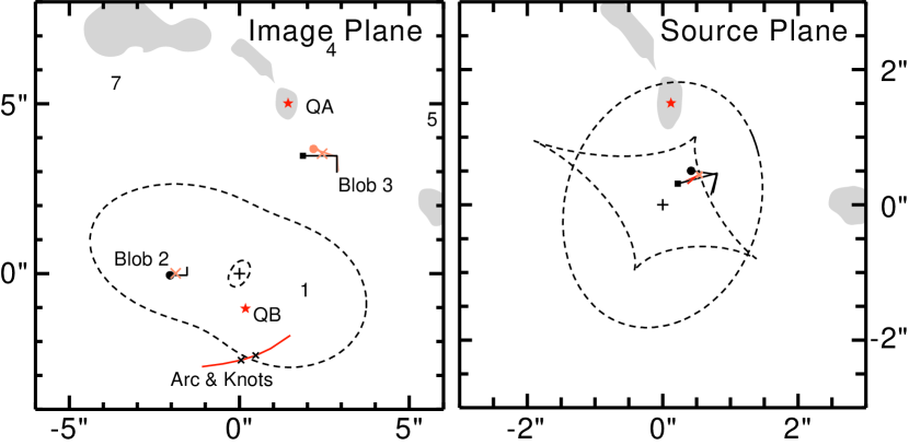
Figure 1: Image (left) and source (right) planes of the 0957+561 lens system under the best-fit C3S+DM1 model described in §4.3.1. Stars mark the positions of the quasar images and source, with the shaded regions outlining the VLA jets. The crosshairs mark the position of the G1 center, and the dashed lines denote the critical lines and caustics of the lens. The source of Blob 2 is schematically illustrated as an “L” shape with a circle at one terminus, whereas Blob 3 is an “L” terminated by a square. The corner of each “L” locates the centroid of its Blob. The arc is a light line segment, including the two Knots ($\times$ symbols). A zoomed view of the Blob and arc sources is given in the middle panel of Figure 4. In the Image Plane, the predicted locations for two counterimages of the Knots are marked as light crosses atop Blobs 2 and 3; the predicted counterimage of Blob 2 is shown also atop Blob 3. The sources for both Blobs and Knots are astride the caustic, with the arc source being very compact. A highly demagnified quasar image is predicted near G1 but not shown here. Numerals in the image plane denote the other HST Blobs, which are not multiply imaged.

With a good model in hand we now can proceed to bound the acceptable range in $\Delta\hat{t}$. With $\theta_{\sigma}$ restricted to the NE quadrant, the best-fit model has $\Delta\hat{t}=10.87$ and the widest range within the 95% CL bounds ($\chi^{2}<9.48$ for 4 DOF) is $9.89<\Delta\hat{t}<11.94$. The parameters which extremize $\Delta\hat{t}$ are listed in Table 4.3.1.

The highest value for $\Delta\hat{t}$ requires a G1 ellipticity set to the a priori upper bound of $e=0.6$ (axis ratio 2:1). Removing this restriction results in an upper bound on $\Delta\hat{t}$ only 0.3% higher (at $e=0.62$), so the upper limit on H₀ is not really set by the 2:1 axis ratio criterion.

The search for minimal $\Delta\hat{t}$ yields a model with G1 orientation of $PA\approx 40\arcdeg$, which causes the arc source to be “unfolded.” Enforcing $90\arcdeg\leq PA\leq 180\arcdeg$ (G1 PA in NE quadrant) gives a marginally acceptable arc source, as illustrated in Figure 2. This is admittedly a qualitative judgment. In most of what follows, the models which define the lower bound on $\Delta\hat{t}$ have the same problem of a poor arc source, and we implement the G1 $PA$ restriction to enforce a compact arc source.

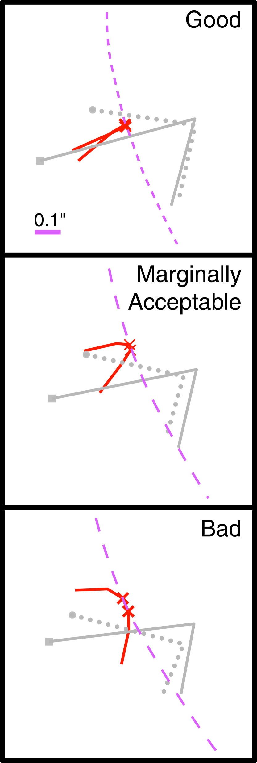
Figure 2: Examples of good, marginally acceptable, and poor sources for the arc. The solid grey “L” with square terminus is the Blob 3 source, while the dotted “L” with circular terminus is the Blob 2 source. The arc is the “U” shape, and the crosses show the source positions for two knots, generally atop the caustic (dashed line). We reject models for which the arc source is more extended than in the middle panel; the bottom panel shows a reject, while the top panel shows precisely the source behavior we would expect.

4.3.2 Adding Cluster Freedom: C3+DM1 (2–4 DOF)

We explore the sensitivity of the allowable $\Delta\hat{t}$ range to the details of the cluster third derivatives by changing the restrictions in Equation (17) that relate the third-derivative cluster terms. We discover that our results are insensitive to the relations assumed among the third-derivative terms. This means that our results should be robust to ellipticity or irregularity in the shape of the cluster dark matter.

We first set $\sigma=0$. The best-fit model has $\chi^{2}/\nu=5.57/4$ ($Q=0.23$), with a 95% CL range ($\chi^{2}\leq 9.48$) of $9.88<\Delta\hat{t}<11.97$. This is nearly identical to the $\Delta\hat{t}$ range for the previous model (C3S+DM1).

Next we set $\delta=0$. The best-fit model has $\chi^{2}/\nu=7.27/4$ ($Q=0.12$), with a 95% CL range ($\chi^{2}\leq 9.48$) of $9.84<\Delta\hat{t}<12.37$ (assuming $\theta_{\sigma}$ in the NE quadrant).

Adding the $m=3$ term ($\delta$) yields a somewhat better fit than does the $m=1$ ($\sigma$) term. But adding either term to the lens model vastly improves the fit over the quadratic-order cluster models. Without these C3 terms, all of the lensing potential has even-$m$ symmetry about G1. It seems that the key to a satisfactory fit is an odd-$m$ term to break the inversion symmetry in the potential.

We can give the cluster more freedom by allowing all four parameters of the third-order cluster potential to be free, leaving 2 DOF for the fit. A marginally acceptable fit is attainable ($\chi^{2}/\nu=5.57/2$), and models within the 95% CL level ($\chi^{2}\leq 6.00$) produce $10.44\leq\Delta\hat{t}\leq 11.31$.

To summarize, varying the restrictions on the cluster third derivatives does not substantially alter the range of H₀ compatible with the observations. Among all C3S+DM1 and C3+DM1 models, the time delay is limited to $9.84<\Delta\hat{t}<12.34$, assuming that the cluster gradient runs to the NE quadrant.

4.3.3 Adding a Stellar Contribution: C3S+ML+DM1 (3 DOF)

Stellar mass is certainly present in G1 so we would like to find good lens models incorporating the ML terms. Indeed a fit with $\chi^{2}/\nu=4.66/3$ ($Q=0.20$) is found, with $b_{\ast}=1.11$. It is comforting that the best-fit value of the mass-traces-light component is quite close to that expected from the stellar population. Furthermore, inclusion of the stellar mass component has not degraded the quality of the fit from the simpler “Best Fit” model of §4.3.1—but it does yield a substantially lower time delay at $\Delta\hat{t}=9.75$ (Table 4.3.1). The DM1 “halo” component is very shallow ($\alpha=-0.56$) and elliptical ($e=0.6$ at $PA=180\arcdeg$) when the ML term is included.

Because the ML term has a strong central mass peak, the dark matter power-law index becomes shallow and the derived $\Delta\hat{t}$ is lowered. The lower limit to $\Delta\hat{t}$ is substantially decreased by including the ML terms: $\Delta\hat{t}=8.70$ is possible at the 95% CL limit of $\chi^{2}=7.81$. This extremal model has the halo index at our a priori limit of $\alpha=-0.5$. Shallower values of $\alpha$ would produce even lower H₀ values with good fits to the lensing geometry.

Addition of a finite core radius to the dark matter (C3S+ML+CORE) results in fits optimized at zero core radius, and no expansion of the allowed range of $\Delta\hat{t}$.

4.3.4 Adding Central Black Hole: C3S+BH+ML+DM1 (2 DOF)

The addition of a black hole constrained to $M_{9}<10$ does not qualitatively change the fits. It does, however, allow $\Delta\hat{t}$ values as low as 8.46 within the 95% CL contours ($\chi^{2}/\nu<6.00/2$), a 3% reduction in H₀. For this new extremal model, the black hole mass is at its a priori upper limit, and the dark matter halo is again as shallow as our a priori limit of $\alpha\leq-0.5$ allows. This is the lowest value of $\Delta\hat{t}$ found in any of our models, so we refer to this as the “Minimal H₀” model. Its parameters are in Table 4.3.1 and its radial profile is plotted in Figure 3.

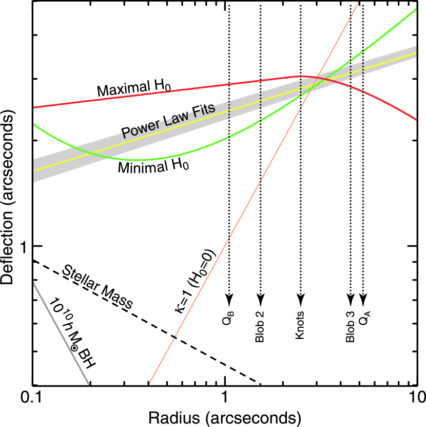
Figure 3: Radial mass profiles of several models for the 0957+561 lens. The vertical axis is the effective deflection angle $M(<R)/\pi R$ vs $R$, with $M(<R)$ being the mass (in critical units) projected within radius $r$ of the center of G1. An isothermal profile is horizontal in this plot. The 95% CL range of power-law galaxy models (C3S+DM1, §4.3.1) is denoted by the gray band, and the best-fit model (with $\Delta\hat{t}=10.9$) runs along this band. A much broader range of H₀ values is found if we allow the mass profile to be more complex than a power law. The “Maximal H₀” model ($\Delta\hat{t}=14.1$) has two power-law segments (C3S+DM2, §4.3.5), and the “Minimal H₀” model ($\Delta\hat{t}=8.5$) has power-law dark matter with black hole and stellar mass terms added (C3S+BH+ML+DM1, §4.3.4). The deflection due to a $10^{10}h^{-1}M_{\odot}$ black hole and to the expected stellar mass are shown near the bottom. These profiles are all plotted assuming ${\bar{\kappa}_{30^{\prime\prime}}}=0$; increasing ${\bar{\kappa}_{30^{\prime\prime}}}$ will drive the radial profile toward the “$\kappa=1$” line, and also drives the derived H₀ toward zero. It is apparent that H₀ is determined largely by the slope of the mass profile between the radii of the two quasar images (as marked). The arc/Blob objects at the marked intermediate radii help constrain the mass profile, but it is clear that models restricted to a single power law G1 profile do not sample the full allowed H₀ range.

Thus we see that the addition of the centrally concentrated stellar and black-hole masses has weakened the lower bound on H₀ by 15%, an appreciable change. The lower bound on H₀ also depends strongly on our a priori limit on the dark matter radial index: adopting the stricter limit of $\alpha<-0.6$ brings the 95% CL lower limit on $\Delta\hat{t}$ back up 7% to 9.10.

4.3.5 Two-Segment Power Laws: C3S+DM2 (0 DOF)

We give G1 substantially more freedom with the DM2 model. With the C3S cluster model we formally have zero degrees of freedom in the fit, but we will judge these models as if they have $\nu=1$. Allowing such freedom expands the range of $\Delta\hat{t}$ compatible with the lensing constraints.

Pushing down the lower bound of $\Delta\hat{t}$ we find models with very shallow G1 mass: $\alpha_{0}=-0.75$, $r_{01}=0\farcs 9$, and $\alpha_{1}=-0.5$. The minimum time delay value within the 95% CL bound of $\chi^{2}\leq 3.81$ is $\Delta\hat{t}=7.36$, another 15% decrease from the lower limit in the previous section. This model is not, however, astrophysically plausible, because its surface mass density inside $r\approx 0\farcs 2$ is only slightly above the minimum expected from the stellar mass [cf. Equation (15)], and is quite shallow. The dark matter density would then have to be decreasing toward the core, which we regard as unlikely. We can include an ML term with $b_{\ast}=1$ to enforce a density everywhere at least as large as the expected stellar contribution, and require (as usual) that the dark matter component increase toward the center. The model of this type with lowest attainable $\Delta\hat{t}$ within the 95% CL contours turns out to be virtually indistinguishable from the lowest-$\Delta\hat{t}$ C3S+BH+ML+DM1 model found above. The additional freedom for G1, therefore, does not extend the lower bound on H₀ if we use the stellar mass as a floor for the G1 mass.

The upper bound on $\Delta\hat{t}$ is raised to 14.10 by C3S+DM2 models which let G1 break from a nearly-isothermal slope of $\alpha_{0}=-0.93$ to a steeper $\alpha_{1}=-1.5$ outside of $r_{01}=2\farcs 2$. This bound is 13% higher than those derived in the previous sections, and is the “Maximal H₀” model in our study. The H₀ bound is this time strongly dependent upon our a priori limit of $\alpha>-1.5$ on the steepness of the G1 profile. Since the Tonry & Franx (1998) stellar dynamics measurements only extend to $\pm 3\arcsec$ it is not likely that their observations can rule out this mass model. Perhaps by comparing with studies of other ellipticals one could exclude this mass distribution for G1, but for now we are forced to accept this as a valid model.

4.4 Fourth-Order Cluster Models

An extension of the approximation for the cluster potential from quadratic order to cubic order has greatly improved the fit to the observations. We have seen that the $\Delta\hat{t}$ values are not very sensitive to the precise form of the cubic terms, but we would also like to see if our results on H₀ are robust against cluster potential terms beyond cubic order.

4.4.1 Peaked Cluster: C4P+DM1 (3 DOF)

We might expect a gentle peak in the cluster mass near G1 to decrease the lower bound on $\Delta\hat{t}$ by adding a nearly-constant mass sheet to the vicinity of the quasar images. Including the C4P mass term from Equation (18), however, does not lead to any expansion of the allowed $\Delta\hat{t}$ range, and the best-fit models place $\kappa_{p}=0$. Significant values ($\kappa_{p}\gtrsim 0.1$) are strongly excluded by the strong lensing constraints. We conclude that the cluster mass does not have an important maximum within $R=30\arcsec$, in mild disagreement with the weak-lensing analysis of Paper I.

4.4.2 Quartic Cluster: C4S+DM1 (2 DOF)

The C4S restricted fourth-order cluster approximation has 6 free parameters (§3.5.4), so we will combine it with the simplest mass model for G1, the elliptical power-law DM1. More complex models for G1 would leave insufficient degrees of freedom. We limit the amplitude $c_{4}$ of the quartic cluster terms to the value they would acquire from a singular isothermal cluster located only 10″ away from the center of G1. Larger values than this would make the cluster mass supercritical within the central 10″ region, which is clearly not the case. We also require the quartic terms to point roughly toward the NE, $90\arcdeg<\theta_{4}<200\arcdeg$.

The C4S+DM1 model does have an acceptable best fit, with $\chi^{2}/\nu=4.33/2$ ($Q=0.11$). The parameters are similar to those of the best-fit C3S+DM1 model. The range of time delays attainable within the 95% CL region ($\chi^{2}\leq 6.0$) are $9.71<\Delta\hat{t}<12.47$. Recall from §4.3.1 that the acceptable range for the C3S+DM1 models was $9.89<\Delta\hat{t}<11.94$. So the addition of the fourth-order cluster terms does not improve the quality of the fit to the observations, and permits an extension of the allowed $\Delta\hat{t}$ (and hence H₀) range of only +4% or -2%, a small fraction of the total allowed range. Unless the cluster mass has strong features on scales of $\sim 10\arcsec$ or less, further terms in the power-law expansion of the cluster potential should have even smaller effects on lens models. Thus we can conclude that, given the current set of lensing constraints, the cubic approximation to the cluster is necessary and sufficient for the purposes of placing bounds on H₀.

4.5 Overview of Strong-Lensing Models

We summarize here the properties of the various lens models we have tested against the observations.

• It is not possible to fit the observed lensing geometry with astrophysically reasonable models that use the quadratic (C2) approximation to the cluster potential. All such models, with up to 12 free parameters, are excluded at $>97\%$ confidence. There is good agreement among various authors on the parameters of the best-fitting simple models, though it is clear that the real lens is not as simple as these models.

• Allowing third-order terms in the expansion of the cluster (C3S) potential permits a good fit to the data, even with a single power-law galaxy (DM1). The best-fit C3S+DM1 model has $\chi^{2}/\nu=6.03/4$, a level which occurs by chance with 20% probability. For this simplest, “Best Fit” model, $\Delta\hat{t}=10.9$.

• The fit is insensitive to the details of our restrictions on the cluster third-order terms; a good fit generally seems to need some term that breaks the inversion symmetry of the lens.

• C3+DM1 and C3S+DM1 models with a range $9.84\leq\Delta\hat{t}\leq 12.37$ are consistent with the observations at 95% CL.

• Inclusion of fourth-order cluster terms neither improves the fit nor significantly widens the allowable $\Delta\hat{t}$ range.

• Equally good fits to the data are also available when we include a mass term that traces the light density. The best-fitting models have mass-to-light normalization $b_{\ast}=1.1$, where $b_{\ast}=1$ is what we expect from the stellar population. This agreement is reassuring.

• While inclusion of the stellar mass is not required to fit the lensing geometry, it does yield significantly lower values of $\Delta\hat{t}$ within the 95% CL. The same is true, to a lesser extent, of a central black hole of mass $10^{10}h^{-1}M_{\odot}$. The “Minimal H₀” C3S+BH+ML+DM1 model pushes the lower bound on $\Delta\hat{t}$ to 8.46.

• Allowing the G1 power law to break to a steeper value $\alpha=-1.5$ between the quasars (“Maximal H₀” C3S+DM2 model) raises the upper bound on $\Delta\hat{t}$ to 14.10.

Thus the best-fit simple model gives $\Delta\hat{t}=10.9$, with a 95% CL range of $8.46<\Delta\hat{t}<14.10$. Combining with Equation (10), we have

$$H_{0}=104^{+31}_{-23}\,(1-{\bar{\kappa}_{30^{\prime\prime}}})\;{\rm km}\;{\rm s}^{-1}{\rm Mpc}^{-1}\;\mbox{(95\% CL)}.$$ (27)

We end up, therefore, with a $\pm 20\%$ uncertainty in H₀ from the lens modeling alone. There is additional uncertainty in $1-{\bar{\kappa}_{30^{\prime\prime}}}$, as discussed in the next section. Had we studied only the simplest model that fit the data (C3S+DM1), we would have derived a 95% CL range of smaller than $\pm 10\%$. The additional complexity of the BH, ML, and DM2 terms did not significantly improve the quality of the best fit, but it does more than double the allowed range of H₀. Since these additional terms are astrophysically reasonable, we have no alternative but to consider the more complex models as yielding valid estimates of H₀.

To what extent does the result in Equation (27) depend upon our a priori limitations on the lens mass distribution? The best-fit model, fortunately, does not place any of the model parameters at the a priori bounds. The extremal models, however, place the radial power-law index $\alpha$ of the G1 dark matter distribution at its a priori limits. The lowest-H₀ model, of type C3S+BH+ML+DM1, has $\alpha=-0.5$, and the highest-H₀ model (C3S+DM2) has $\alpha=-1.5$ outside of $r=2\farcs 2$. The bounds on H₀ thus are strongly dependent on our assumptions about a “reasonable” galaxy profile might be. Assuming $\alpha<-0.6$, for example, raises our lower bound on H₀ by 7%, removing one third of the error bar.

The lowest-H₀ model also has the black hole mass at its a priori upper limit of $10^{10}h^{-1}\,M_{\odot}$. A larger value is unlikely, however, and only weakly affects the H₀ bound.

We reiterate as well that we have assumed that the cluster mass gradient points toward the northeast quadrant from G1. Relaxing this constraint would significantly widen the allowed H₀ range.

Figure 3 shows how the radial mass profile is the most important determinant of H₀. We plot the deflection angle $M(<R)/\pi R$ vs $R$, where $M(<R)$ is the mass enclosed within a circle of radius $R$ centered on G1. An isothermal profile is flat in this representation, while a shallower radial mass profile yields an upward slope. We see that the shallower the mass profile between the two quasars, the lower the H₀ value implied. All the valid models cross at a point intermediate to $Q_{A}$ and $Q_{B}$, since the sum of the deflections angles at $Q_{A}$ and $Q_{B}$ must of course equal the 6″ separation between them, as discussed in §3.2.2.

4.5.1 Relation to Previous Models

The inclusion of cluster terms beyond quadratic order dramatically improved the agreement between our lens models and the observed geometry. The models of GN, FGS, and 4 of the 5 BLFGKS models have only a quadratic cluster, which explains why we have found a lower $\chi^{2}$ value for essentially the same constraints. The fifth model of BLFGKS, “FGSE+CL,” includes an elliptical softened-core isothermal G1 and a singular isothermal sphere galaxy cluster. The velocity dispersion and position of the SIS cluster are free parameters, and the cluster potential is exact, not a quadratic approximation. Yet the best-fit $\chi^{2}$ is 41 for 7 DOF, highly excluded.

Our C3S+DM1 model fits the data much better—why? At first glance it might be because we have relaxed the constraint on the position of Jet 5, but in fact we obtain an equally good fit using the error bar on the Jet 5 position given by BLFGKS. The main reason for the improved fit is that we have not required that the cluster have an SIS profile. Indeed the best-fitting model has $\theta_{\gamma}=139\arcdeg$ but $\theta_{\sigma}=169\arcdeg$, meaning that the second and third derivatives of the cluster potential are not aligned, and hence the cluster is not spherical. Furthermore, we have $\gamma=0.14$ and $\sigma=0.015$, whereas an SIS cluster would have $\sigma=\gamma^{2}$. If we take our best-fit C3S+DM1 model and require alignment of $\theta_{\gamma}$ with $\theta_{\sigma}$ to within 5°, the $\chi^{2}$ value rises from 6.0 to 26.7, strongly excluding the alignment that a spherical cluster would generate. An singular isothermal elliptical cluster distribution would require $e\approx 0.5$ to generate the observed 30° misalignment between the mass gradient and the shear. We reiterate that our approach of continuing the power-law approximation to the cluster potential means that we do not have to know or fit the global shape of the cluster, just its multipole moments about G1. We note that it is possible to measure the multipole moments about G1 directly from the shear pattern in a weak lensing map (Schneider & Bartelmann, 1997).

The apparent departure of the cluster from SIS form suggests that it is not safe to infer the $1-\kappa$ factor by assuming that $\kappa=\gamma$, as is done in producing some of the H₀ estimates in BLFGKS.

4.5.2 The Dark Matter Distribution in G1

The strong-lensing models for G1 give detailed information on the mass distribution in the giant elliptical galaxy G1. All of the acceptable lens models share a few characteristics:

• The dark matter distribution is shallower than isothermal within a radius of $\approx 2\farcs 5$. The C3S+DM1 models place the radial index of the total G1 mass at $\alpha=-0.83$. The stellar light distribution is significantly steeper at $-1.9\leq\alpha\leq-1.3$, so when we include a mass-traces-light term in the G1 mass, we find that the remaining mass (“dark” matter) is forced to significantly shallower values of $-0.6\lesssim\alpha\leq-0.5$. The highest-H₀ models have profiles that are nearly isothermal within $2\farcs 5\approx 10h^{-1}$ kpc and significantly steeper beyond this point.

• The total mass surface density is well above the stellar contribution at all projected radii above 0$\farcs$1 (Figure 3).

• The matter distribution is highly elliptical, $0.4\lesssim e\lesssim 0.6$ (axis ratio of 1.5:1–2.0:1), more flattened than the inner isophotes of G1. The dark matter halo is oriented at $160\arcdeg<PA<190\arcdeg$ (measured from East) whereas the isophotes twist from 135° to 145°. Thus the dark matter is out of alignment by 15°–45° from the outer isophotes of the galaxy. Both the ellipticity and position angle of the light tend toward the dark matter values at the outer isophotes (Paper II).

5 Determination of $1-\kappa$

5.1 Choices of Method

With the strong-lensing constraints satisfied, we turn to resolving the sheet-mass degeneracy in these models. Four methods have been used to determine the local density $\kappa_{c}$ of the galaxy cluster near the G1 center:

1. Weak-lensing measurements can measure the mean mass density ${\bar{\kappa}_{30^{\prime\prime}}}$ within the region $R<30\arcsec$ of the G1 center (Paper I). This method has the virtues of being non-parametric, and of measuring precisely the quantity that is needed (the projected mass density). The main drawback at the moment is the undesirably large statistical uncertainty in ${\bar{\kappa}_{30^{\prime\prime}}}$, which we explain below.

2. The line-of-sight velocity dispersion $\sigma$ (LOSVD) of G1 can be measured, providing an absolute normalization of the G1 mass model and hence breaking the sheet-mass degeneracy. The virtue of this method is that the measurement is now quite precise, currently yielding a 95% CL uncertainty of $\pm 12\%$ on the quantity $\sigma^{2}$ that scales H₀ (Tonry & Franx 1998). The drawbacks of this method are that, first, the LOSVD measures a degenerate combination of the G1 mass and the velocity anisotropy of the stars, hence the mass uncertainty is significantly larger than the $\sigma^{2}$ measurement error. Romanowsky & Kochanek (1998) show that incorporation of constraints on the higher-order moments of the velocity distribution can reduce the uncertainty on the G1 mass to $\pm 16\%$ (95% CL) if the three-dimensional structure of G1 potential is known. The second drawback of the LOSVD normalization of $1-\kappa$ is that the LOSVD is sensitive to the three-dimensional structure of the G1 potential whereas the lensing models constrain and require the two-dimensional (projected) mass density of G1. Romanowsky & Kochanek (1998) assumed a spherical G1 mass model from GN; not only do the strong-lensing mass models now require an elliptical projected mass, but the structure along the line of sight is unknown. Allowing these additional freedoms in the orbit modeling will not only greatly complicate the interpretation of the LOSVD data, but would undoubtedly broaden the allowed range of $1-\kappa$. The complications of this interpretation lead us to prefer the weak-lensing method. The surface density implied under the assumption of isotropic orbits does, however, agree well with the weak lensing measurements (Paper I).

3. The velocity dispersion of the galaxies in the G1 cluster can be used to measure the cluster mass density (Garrett et al. 1992; Angonin-Willaime et al. 1994). This method unfortunately suffers the difficulties of both methods (1) and (2) above: the few known members (21) of the G1 cluster poorly determine the cluster $\sigma^{2}$; and the conversion of $\sigma^{2}$ to $1-\kappa$ at the G1 location requires many assumptions about both the three-dimensional shape of the cluster potential and the anisotropies of the galaxy orbits within this potential. It is therefore unlikely that this method will ever approach the precision of the previous two.

4. The properties of the X-ray emitting gas in the cluster potential can be used to normalize a model for its mass (Chartas et al. 1998). This too suffers both from very poor S/N on the relevant measured quantities (X-ray flux, temperature, and core radius) and in the extensive parameterization and implicit assumptions about the physical conditions of the cluster potential and gas within it (e.g. that the cluster is a spherical $\beta$-model with gas in hydrostatic equilibrium). The x-ray data, even with observational improvements, are therefore unlikely ever to provide the best quantitative measure of the sheet mass.

5.2 Weak-Lensing Measurement of ${\bar{\kappa}_{30^{\prime\prime}}}$

In Paper I we use the “aperture massometry” formula of Fahlman et al. (1994) to measure the mean mass density in annuli centered on G1:

$$\bar{\kappa}_{r<r_{i}}-\bar{\kappa}_{r_{i}<r<r_{o}}=r_{o}^{2}\left\langle\gamma_{T}/r^{2}\right\rangle_{r_{i}<r<r_{o}}.$$ (28)

This formula gives the average mass density (in critical units) inside the inner radius $r_{i}$ in term of the average tangential shear component of galaxies $\gamma_{T}$ in some annulus $r_{i}<r<r_{o}$. The formula is exact in the weak lensing limit ($\gamma_{T}\ll 1$), and the second term on the left-hand side reminds us that we measure $\bar{\kappa}_{r<r_{i}}$ only relative to the mean mass density $\bar{\kappa}_{r_{i}<r<r_{o}}$ of the measurement annulus.

Ideally the data can be used directly in Equation (28) to yield the desired ${\bar{\kappa}_{30^{\prime\prime}}}$ at $r_{i}=30\arcsec$. In practice there are four complications: first, the background galaxies are not fully resolved, and the observed shapes are driven toward the shape of the seeing disk, squelching the lensing signal. Second, the source galaxies are at a variety of redshifts, hence the mean critical density (and $\kappa$) may differ by a scaling factor from the value appropriate to the strong-lensing sources at $z=1.41$. In Paper I we measure these scaling factors by creating Monte-Carlo simulations of source galaxies with redshift, shape, and size distributions that match what is known about the true galaxy population. Paper I uses a model of McLeod & Rieke (1995) to estimate a source redshift distribution to $V=26.5$ in an $\Omega=0.1$ Universe; the seeing-corrected $\kappa$ for this population must be increased by $\approx 40\%$ to give the $\kappa$ appropriate to the $z=1.41$ strongly-lensed sources. This scaling factor is uncertain, we estimate, by $\approx 10\%$, due to our ignorance of the galaxy distribution and cosmic geometry. Since the statistical uncertainty in $\kappa$ is much larger ($\approx 30\%$), we will ignore the calibration uncertainties at this juncture.

The third complication in the use of Equation (28) is that the lensing is not entirely in the weak limit. Paper I introduces an iterative approach in which the weak-lensing formula is used to make an initial radial profile, which is then used to apply slight corrections to Equation (28) to account for stronger lensing near the cluster center. As can be seen from the top panel of Figure 6 in Paper I, this introduces only a few percent correction to $\bar{\kappa}_{r<30^{\prime\prime}}$, and the details are not critical here.

The fourth complication is that the data in Paper I extend only to $r_{o}=168\arcsec$, so we must estimate the mean mass density $\bar{\kappa}_{30^{\prime\prime}<r<168^{\prime\prime}}$ before we get a final ${\bar{\kappa}_{30^{\prime\prime}}}$. Paper I derives this correction by assuming that the cluster follows an isothermal profile at radii beyond the outer bound of the data. The second (annular) term on the left-hand side, $\bar{\kappa}_{30^{\prime\prime}<r<168^{\prime\prime}}$, is 22% of the desired ${\bar{\kappa}_{30^{\prime\prime}}}$ term under this assumption. In essence we are still subject to a sheet-mass degeneracy, although this time the sheet must be constant across a 168″ radius instead of the much smaller strong-lensing region. When smoothed over this much larger circle, the expected $\bar{\kappa}$ from the cluster is far smaller, and thus so is its uncertainty. We will ignore the uncertainty in this 22% correction, and take the value derived from the isothermal approximation in Paper I.

The mean mass density measured from weak lensing can be read from Figure 6 in Paper I (where the lower panel incorporates the small correction for departure from weak lensing). Correcting to the critical density appropriate for our $z=1.41$ strong-lensing sources, we obtain

$${\bar{\kappa}_{30^{\prime\prime}}}=0.26\pm 0.08.$$ (29)

This is the 1-sigma random error due to the “shape noise” of the intrinsic ellipticities in the finite number of background galaxies. Since the S/N ratio on this quantity is only 3.2, we can ignore for the time being the calibration errors relating to the source redshift distribution and the mass density beyond $r_{o}=168\arcsec$.

The weak lensing data thus yield $1-{\bar{\kappa}_{30^{\prime\prime}}}=0.74\pm 0.16$ (95% CL). Note that the fractional error on $1-\kappa$ is smaller than the fractional error on $\kappa$. This helps the error budget a bit, but the statistical error induced on H₀ is still $\pm 22\%$ at the 95% CL. Combining this weak-lensing result with the results of strong-lensing models of Equation (27) gives the value of the Hubble constant:

$$H_{0}=77^{+29}_{-24}\;{\rm km}\;{\rm s}^{-1}{\rm Mpc}^{-1}\;\mbox{(95\% CL)}.$$ (30)

We caution the reader that the probability distribution for H₀ within these bounds is not Gaussian; for example, the best-fitting models span the range 65–80 ${\rm km}\,{\rm s}^{-1}\,{\rm Mpc}^{-1}$, with all having essentially the same likelihood.

6 Prospects for Improvement

The H₀ from the 0957 time delay derived in Equation (30) is disappointingly imprecise, with a $\pm 30\%$ 95% CL range that encompasses nearly all other current estimates of H₀. This uncertainty is due in equal parts to remaining freedom in the strong-lensing model of the G1 mass distribution and to statistical uncertainty in the weak-lensing measurement of $1-\kappa$ (our weak lensing aperture of $R=30\arcsec$ was chosen to make this the case). Substantial improvement in the precision of the H₀ estimate will therefore require improvements in both aspects of the problem. We believe that imminently available data will permit these improvements.

6.1 Tighter Strong Lensing Constraints

We could set tighter bounds on H₀ if we could independently constrain the mass profile of G1. Measurements of the LOSVD (and other moments of the velocity) can do this. The analysis will not be straightforward because of the reasons mentioned in §2.

Deeper imaging of the 0957 lens system could also very easily narrow the $\pm 20\%$ modeling uncertainty in H₀. The arc and Blobs 2 & 3 are images of a common source object. The WFPC image in Paper II has insufficient S/N to see the morphology of these objects. A deeper image would allow us to create a precise correspondence between different components of these images, thus further constraining the models. Figure 4 shows the relative source-plane positions of the arc and Blobs in the best-fit and H₀-extremizing models. We see that a detailed view of where the arc/Knot source lies within the Blobs could distinguish these models. Deep STIS observations of this system obtained in March, 1999 should provide the S/N level required.

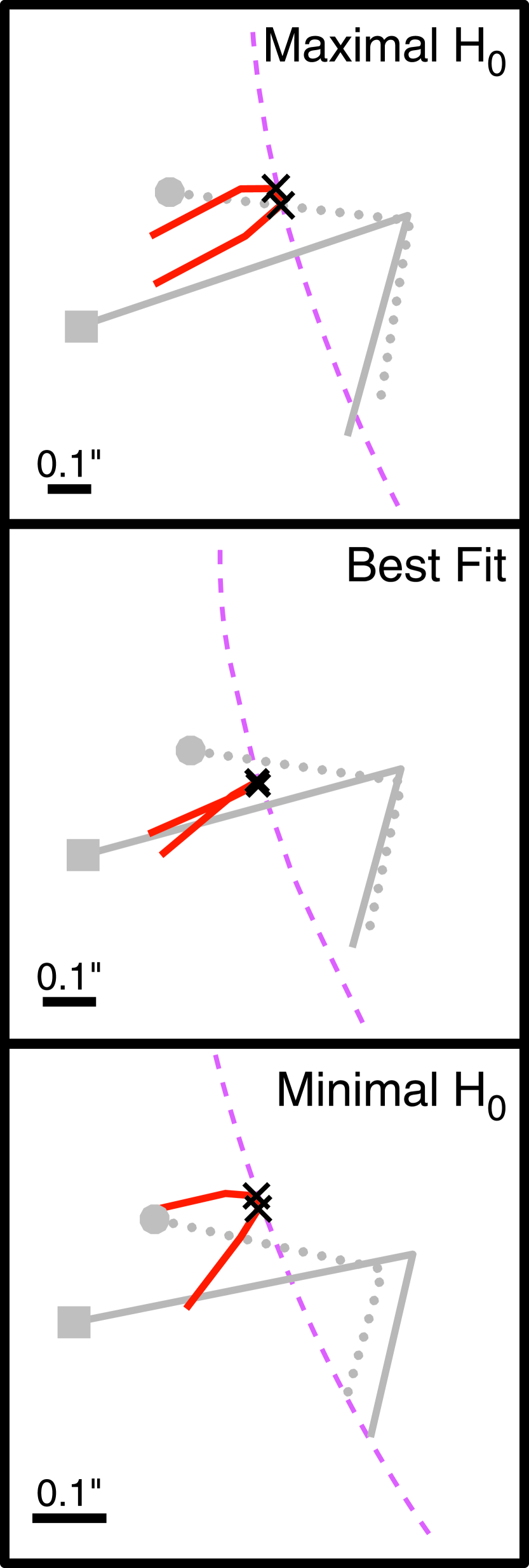
Figure 4: Closeup of relative source-plane positions of Blob 2, Blob 3, and the arc in the best-fit model and the two models which extremize H₀. All symbols have the same meaning as in Figure 2. Recent STIS observations of the system provide high-S/N images of these objects, which should allow us to determine the proper source-plane configuration.

We believe it to be quite likely that additional multiply-imaged features will be discovered either in our recent STIS observations of 0957, in the existing NICMOS images of the system (Kochanek et al. 1998), or in future radio imaging. This would help pin down the radial mass profile and decrease the H₀ uncertainty due to the modeling.

6.2 Tighter Weak Lensing Constraints

The weak-lensing measure of ${\bar{\kappa}_{30^{\prime\prime}}}$ is limited primarily by statistical fluctuations in the shapes of the observed galaxies. Improvement is possible if an image of the field can be obtained with a higher density $n_{g}$ of resolved galaxies at S/N$\gtrsim 10$. The uncertainty in ${\bar{\kappa}_{30^{\prime\prime}}}$ scales as $n_{g}^{-1/2}$. The ${\bar{\kappa}_{30^{\prime\prime}}}$ measurement in Paper I uses 67 galaxies per square arcmin at $24<V<26.5$, many of which are poorly resolved even in the excellent seeing (FWHM of 0$\farcs$6) of the CFHT image. The image is not particularly deep, having been obtained with a front-illuminated CCD; a higher $n_{g}$ over a larger field could be obtained with currently-available thinned CCDs. Even more promising is the use of the Hubble Space Telescope; even relatively short (3600 s) exposures with the WFPC2 camera yield arclet densities of $n_{g}\approx 50\;{\rm arcmin}^{-2}$ (Hoekstra et al. 1998), with essentially all being completely resolved. A mosaic of deeper WFPC2 images, or, even better, a few images from the upcoming Advanced Camera imager, would allow a large increase in $n_{g}$ and hence in the precision of ${\bar{\kappa}_{30^{\prime\prime}}}$.

Improved S/N in the weak lensing data will also help refine the strong lensing model, since the arclets can be used to quantify the multipole moments of the mass distribution both internal and external to the $R=30\arcsec$ division that we have placed between the weak and strong lensing regions (Schneider & Bartelmann 1997). The present data are not sufficiently accurate to yield useful constraints beyond the monopole moment ${\bar{\kappa}_{30^{\prime\prime}}}$.

7 Conclusions

We have pursued the goal of an independent, global, conceptually simple measure of H₀ via the time delay of the gravitational lens 0957+561. The simplicity is lost, however, as we delve into the messy consideration of realistic models for the mass distribution in the lens. Despite the accuracy of the time delay measurement, indeterminacy in the G1 mass model and the cluster mass each add $\pm 20\%$ uncertainty to the value of H₀, with our final determination being $H_{0}=77^{+29}_{-24}$${\rm km}\,{\rm s}^{-1}\,{\rm Mpc}^{-1}$ (95% CL). While the resultant accuracy of our H₀ value is disappointing, the good news is that we have, for the first time, produced a lens model that accurately reproduces the many observed features of this lens.

Our investigation of an extensive variety of lens models shows that the G1 lens must be elliptical and must be shallower than isothermal, and the surrounding cluster must be considered in more detail than a constant magnification and shear, and the cluster must depart from circular symmetry. The G1 lens mass profile can be a simple power law, but a much wider range of H₀ values are accessible if we allow the mass profile the freedom to depart from a single power law. In particular, the inclusion of a mass component that traces the light in G1, with a M/L ratio as expected from the stellar population, leads to a lowered value of H₀. The range of allowed H₀ depends strongly on the a priori limitations placed upon the G1 mass profile.

Constraining the lens with only the two-image system (quasars and jets) gives an extremely wide range of possible H₀ values (Kochanek, 1991) unless one artificially restricts the G1 mass distribution to circular or isothermal profiles. The 0957 system now also includes a likely four-image system (arc & Blobs) at a variety of radii from the G1 center, which reduces the H₀ uncertainty from modelling to $\pm 20\%$ under our broad range of possible G1 models. Additional multiply-imaged sources would curtail this freedom substantially.

The mass-sheet degeneracy from the surrounding cluster is broken in a straightforward, non-parametric fashion with the weak lensing data of Paper I. Improvements to this measurement require only deeper high-resolution images. LOSVD measurements of G1 can also break the mass-sheet degeneracy, but this will require dynamical modelling of realistic (e.g. elliptical, non-isothermal) potentials.

We believe that the uncertainties on H₀ from this system will be cut in half within a year or so. But 0957+561 is now only one of three gravitational lenses useful for H₀ determination: PG 1115+080 (Schechter et al. 1997, Barkana 1997) and B0218+357 (Biggs et al. 1999) both now have accurately determined time delays, and known redshifts for both source and lens galaxies. Resultant values of H₀ have already been published for each: $H_{0}=44\pm 8$ (isothermal lens) or $H_{0}=65\pm 10$ (mass-traces-light lens) for PG1115 (Impey et al. 1998), and $H_{0}=69^{+13}_{-19}$ for B0218 (Biggs et al. 1999), each at 95% CL in the usual units. While these lenses would seem to offer higher precision on H₀ than the result derived for 0957 in this paper, we believe that the claimed precision on H₀ is overestimated because the lenses have as yet been modelled only with relatively simple mass distributions—isothermal ellipsoids. While the lens observations may be well fit by these simple models, this does not exclude the possibility that the mass distribution may take other sensible forms. In the case of 0957, we found the lens well fit by the C3S+DM1 power-law ellipsoid, but the allowed H₀ range is much larger when we allow additions such as the mass-traces-light component.

It has been claimed that the 4-image systems such as PG1115 will offer better H₀ constraints than 2-image systems such as 0957 or B0218. We have seen, however, that the 0957 model is now constrained by a 2-image and a 4-image system and still has 20% uncertainty in H₀ from the G1 mass model. A competitive measure of H₀ will apparently require even more constraint on the lensing geometry. For 0957+561, it is likely that other multiply-imaged background sources will be found in deep images, but this is less likely for the other systems simply because their strong-lensing regions are smaller (Einstein-ring radii of 3″ for 0957, 1$\farcs$1 for PG1115, and 0$\farcs$17 for B0218). Fortunately there is hope because all three systems now show ring-like images of the quasar host system: 0957 and PG1115 from NICMOS images (Impey et al. 1998; Kochanek et al. 1998) and B0218 in radio images (Patnaik et al. 1993). In theory, a high-S/N image of a well-resolved ring with extended structure can offer very strong constraints on the mass model (see method of Wallington et al. 1996). At present, however, such information has not yet been used in detailed modelling of any of these systems (indeed the S/N of present ring images may be insufficient). So we reiterate our caution: the 0957 system currently has many more quantitative constraints on lensing geometry than either PG1115 or B0218, and yet a realistic examination of possible mass distributions leaves H₀ uncertain by $\pm 20\%$, even ignoring the uncertainties in $1-\kappa$.

Half of our H₀ error budget arises from uncertainties in $1-\kappa$, which is a substantial correction for 0957 because the lens is in a modest cluster. Will other lenses be free of errors arising from the mass-sheet degeneracy? In the case of PG1115, it is clear that the lens galaxy is in a group, and the influence of the group potential is important for the lens model (Impey et al. 1998), so the mass-sheet term (and higher-order “cluster” potential terms) must be considered in a thorough examination of the lens model. We note that the precision of weak lensing and LOSVD measurements in determining $\kappa$ are independent of the value of $\kappa$, so the mass sheet problem may be no more accurately resolved in PG1115 than in 0957, despite the fact that the mass sheet is weaker. For B0218, which appears to be an isolated spiral, there may be a priori reasons why $\kappa$ can be assumed to be close to zero, and it need not be measured accurately by weak lensing or LOSVD.

We have introduced unpleasant but realistic complexity and uncertainty into the determination of H₀ via gravitational time delays. We consider this a sign of the maturity of the field rather than a discouragement of further investigation, though, since we believe that each lens will be left with $\approx 10-15\%$ uncertainty in H₀ once detailed lens models incorporating a variety of lensed features are produced for each lens. Since the errors in each case are independent, the increasing numbers of systems with known time delays will continue to yield a more accurate average H₀ value. We reiterate the virtues of the lensing H₀: it is a global measurement of geometry, not affected by local anomalies of flow or expansion; it is physically based, so that it is difficult to imagine any undetected systematic effects that might affect its results, aside from a failure of General Relativity. Finally, it is completely independent of other methods, and the continued agreement with these other methods increases confidence in the entire distance ladder.

Appendix A Justifications for De-Emphasizing Jet Precision

The positions of components A5 and B5 are determined to high precision, with formal uncertainties of only $\approx 0.1$ mas, or 0.2% of their displacements from the quasar cores. Use of these tiny uncertainties in our fitting procedure would effectively constrain the local magnification matrices (second derivatives of the lens potential $\phi$) to 0.2%. We choose to relax this constraint by increasing the sizes of the error ellipses for the jet image positions to circles with radii equal to 1% of their displacements from the quasar cores. There are several justifications for this:

• The 0.1 mas formal uncertainties given by the VLBI analyses may be underestimated. The A5/B5 positions change by $\approx 0.3$ mas for BLFGKS’s various modelling procedures, which we take as more indicative of the uncertainty. The complex structures of the jets are being fit by a simplified model of a chain of Gaussians. The fitted locations of these idealized jet components probably is somewhat dependent upon the $uv$-plane coverage (e.g. the effective resolution) of the observations, and perhaps the S/N level. Since the B jet is a demagnified version of the A jet, it is effectively being viewed with different $uv$-plane coverage (relative to its angular size) than the A jet. It might therefore be imprudent to trust the relative positions of the A and B Gaussian components to the formal 0.1 mas error.

• The quantity of interest to us is the gravitational potential difference between quasars A and B, which is a large-scale property of the lens. Requiring jets A5 and B5 to have a common source is in essence a constraint upon the magnification near the A and B quasars, which depends primarily on the lens mass density at A and B image locations. Specifying such a local property as tightly as 0.1% could misleadingly constrain the global solution for the G1 mass parameters, if the parameterized form of the mass distribution does not exactly match the true distribution. It is unlikely that any simple parametric model of the G1 mass would describe the true mass distribution to better than 1% accuracy on 50 mas scales. We consider it prudent, therefore, to increase the uncertainties in jet positions, thereby allowing the models some freedom in local magnification, which allows for the possibility that the true surface density has small-scale deviations from our model.

• Increasing the error ellipse on the jet components can only increase the range of H₀ values from models with acceptable $\chi^{2}$ values. Our approach is therefore the conservative one with regard to constraining H₀.

Appendix B Potentials for Elliptical Power-Law Mass Distributions

We wish to calculate the potentials and its derivatives for power-law elliptical mass distributions as described by Equations (12). We choose to expand the mass distribution into a multipole series, each term of which has easily derived and rapidly calculable potential and derivatives. We define

$$\Sigma(r,\theta)/\Sigma_{\rm crit} = br^{\alpha}\left[1-e\cos 2(\theta-PA)\right]^{\alpha/2}(1-e^{2})^{-\alpha/4}$$ (B1)

$$\equiv \sum_{m=0}^{\infty}a_{m}(e,\alpha)r^{\alpha}(1-e^{2})^{-\alpha/4}\cos\left[2m(\theta-PA)\right]$$

$$\Rightarrow\qquad a_{m}(e,\alpha) = {2b\over\pi}\int_{0}^{\pi}(1-e\cos 2\theta)^{\alpha/2}\,\cos 2m\theta\,d\theta\qquad(m>0).$$

Expanding the parentheses under the integral as a power series in $e$ we obtain

$$\qquad a_{m}(e,\alpha)={2b\over\pi}\sum_{j=0}^{\infty}\left[{{(-e)^{j}}\over{j!}}{{(\alpha/2)!}\over{(\alpha/2-j)!}}\int_{0}^{\pi}\cos^{j}2\theta\,\cos 2m\theta\,d\theta\right]$$ (B2)

for $m>0$. The integral vanishes unless $j-m$ is even and positive, in which case

$$\int_{0}^{\pi}\cos^{j}2\theta\,\cos 2m\theta\,d\theta={{\pi j!}\over{2^{j}\left({{j-m}\over 2}\right)!\left({{j+m}\over 2}\right)!}}$$ (B3)

Defining $2k\equiv j-m$ and $\gamma\equiv-\alpha/2$, the above two equations may be combined to give

$$a_{m}(e,\gamma)={{be^{m}}\over{2^{m-1}}}\sum_{k=0}^{\infty}\left({{e^{2}}\over 4}\right)^{k}{{(\gamma+m+2k-1)!}\over{(\gamma-1)!k!(k+m)!}}\qquad(m>0).$$ (B4)

For $m=0$ there is an additional factor of 2. Successive summands are easily computed by recursion and the sum converges rapidly for small $e$. Even for $e\gtrsim 0.5$ convergence is rapid beyond $k\sim m$. Substituting the coefficients Equation (B4) into the multipole sum in Equation (B1) gives our expression for the power-law ellipse surface density. In practice we find that carrying multipoles up to $m=3$ and the expansion of multipole coefficients to order $e^{6}$ describes the surface density to 1% accuracy even at our most difficult limits of $\alpha=-1.9$ and $e=0.6$.

With the density expanded as multipole moments, the solution for the potential is straightforward. We assume that the mass distribution is described by Equation (B1) between radii $r_{-}$ and $r_{+}$. Each term in the dimensionless surface density of the form

$$a_{m}r^{\alpha}\cos[2m(\theta-PA)]$$ (B5)

gives rise to a term in the potential of the form

$${{a_{m}}\over{2m}}\cos[2m(\theta-PA)]\left\{\begin{array}[]{rrrc}{{r_{-}^{\alpha+2-2m}-r_{+}^{\alpha+2-2m}}\over{\alpha+2-2m}}r^{2m}&&&r<r_{-}\\[3.0pt] {{-r_{+}^{\alpha+2-2m}}\over{\alpha+2-2m}}r^{2m}&+\;{{4m}\over{(\alpha+2)^{2}-4m^{2}}}r^{\alpha+2}&+\;{{r_{-}^{\alpha+2+2m}}\over{\alpha+2+2m}}r^{-2m}&r_{-}<r<r_{+}\\[3.0pt] &\lx@intercol\hfil{{r_{-}^{\alpha+2+2m}-r_{+}^{\alpha+2+2m}}\over{\alpha+2+2m}}r^{-2m}\lx@intercol&r>r_{+}\end{array}\right.$$ (B6)

This equation breaks down for $\pm 2m=2+\alpha$, but if we restrict our galaxy profiles to $-2<\alpha<0$ there will be no difficulties. The analytic derivatives of $\phi$ with respect to the $x$ and $y$ coordinates are then easily calculated.

Appendix C Surface Density of Stellar Component of G1

Equation (15) describes a surface mass density for G1 that traces its observed surface brightness distribution. Here we derive the scale factor between the mass and luminosity distributions that we should expect for an old stellar population.

The observed F555W ($=V$) filter band has a central wavelength of 408 nm in the $z=0.36$ rest frame of G1, very close to the nominal $B$-band central wavelength of 445 nm. We can therefore estimate $S\!B_{B,0}$, the rest-frame B-band surface brightness, and be insensitive to assumptions about the source spectrum. This is given by

$$S\!B_{B,0}=S\!B_{V}-K_{V}(z=0.36)+(B-V)_{0}-10\log(1+z),$$ (C1)

where $S\!B_{V}$ is the observed $V$-band surface brightness, $K_{V}$ is the $K$-correction in $V$ band for redshifting the spectrum to $z=0.36$ (as defined in Coleman, Wu, & Weedman 1980), and $(B-V)_{0}$ is the color the galaxy would have if viewed in its rest frame. For the spectrum of a present-day elliptical galaxy, $K_{V}(z=0.36)+(B-V)_{0}=-0.16$ from values in Coleman, Wu, & Weedman (1980) or $-0.14$ from values in Fukugita et al. (1995). As expected these agree quite well since the transformation is nearly independent of source spectrum, and we will take $K_{V}(z=0.36)+(B-V)_{0}=-0.15$ for the G1 rest-frame spectrum (which will be of a younger population than a present-day elliptical).

Given the rest-frame surface brightness, the surface mass density can be expressed in terms of the $B$-band mass-to-light ratio (in solar units) $\Phi_{B}$:

$$\Sigma_{\ast}=\Phi_{B}10^{-0.4(S\!B_{B,0}-B_{\odot})}{{M_{\odot}}\over{(10\,{\rm pc})^{2}}}\left({{1\,{\rm rad}}\over{1\arcsec}}\right)^{2}.$$ (C2)

Combining Equations (2), (C1), and (C2), $B_{\odot}=5.51$, and the above-mentioned color and $K$ corrections yields

$${\Sigma_{\ast}\over{\Sigma_{\rm crit}}} = \Phi_{B}10^{-0.4(S\!B_{V}-K_{V}(z=0.36)+(B-V)_{0}-B_{\odot})}(1+z)^{4}{{4\pi GM_{\odot}}\over{c^{2}}}{{D_{OL}D_{LS}}\over{D_{OS}(10\,{\rm AU})^{2}}}$$ (C3)

$$= \Phi_{B}h^{-1}10^{-0.4(S\!B_{V}-19.46)}.$$

We have as usual taken $H_{0}=100h\,{\rm km\,s^{-1}\,Mpc^{-1}}$, and have assumed $\Omega=1$, $\Lambda=0$. For an open cosmology the answer is 10% higher, while it can rise by 60% for a $\Lambda$-dominated Universe.

What value is expected for $\Phi_{B}$? The synthesized old stellar populations of Worthey (1994) with $[{\rm Fe}/{\rm H}]=0.25$ have $\Phi_{B}=0.62\,T_{\rm Gyr}$ to within a few percent (with $T_{\rm Gyr}$ the age of the Universe in Gyr). Changing the metallicity to 0 or 0.5 changes $\Phi_{B}$ by -25% or +10%, respectively, so we will place a $\pm 20\%$ uncertainty on this value. In an $\Omega=1$ cosmology, the age of the Universe at $z=0.36$ is $4.2h^{-1}$ Gyr. This age can be higher for open or $\Lambda$-dominated Universes. The resultant estimate for $\Phi_{B}$ of the G1 stellar population is $\Phi_{B}=2.6h^{-1}\pm 20\%$ ($\Omega=1$). Using $S\!B_{V}=22.4$ at $r=1\arcsec$ (Paper II), we obtain

$${\Sigma_{\ast}\over{\Sigma_{\rm crit}}} = 10^{-0.4(S\!B_{V}-20.5)}h^{-2}$$ (C4)

$$= (0.17\pm 0.03)h^{-2}\qquad(r=1\arcsec,\,\Omega=1).$$

The highest anticipated $h$ is 0.8 , and we must remember that the mass density in Equation (15) will be scaled by $1-\kappa_{c}\approx 0.7$ [Equation (6) and §5.1]. We then arrive at the prefactor of 0.16 in Equation (15) as the value we expect from the stellar population of G1. This minimum value might be lowered if the mean metallicity is solar or below; the minimum value can be up to twice as large if the Universe is dominated by a cosmological constant or if $h=0.5$.

References

- (1) Angonin-Willaime, M.-C., Soucail, G., & Vanderriest, C. 1994, A&A, 291, 411
- (2) Avruch, I. M., Cohen, A. S., Lehár, J., Connor, S. R., Haarsma, D. B., & Burke, B. F. 1997, ApJ, 488, L121
- (3) Bernstein, G. M., Tyson, J. A., & Kochanek, C. S. 1993, AJ, 105, 816
- (4) Barkana, R. 1997, ApJ, 489, 21
- (5) Barkana, R., Lehár, J., Falco, E. E., Grogin, N. A., Keeton, C. R., & Shapiro, I. I. 1998, astro-ph/9808096.
- (6) Bernstein, G., Fischer, P., Tyson, J. A.,& Rhee, G. 1997, ApJ, 483, L79 (Paper II)
- (7) Biggs, A. D., Browne, W. A., Helbig, P., Koopmans, L. V. E., Wilkinson, P. N., & Perley, R. A. 1999, MNRAS, 304, 349.
- (8) Chartas, G., Falco, E., Forman, W., Jones, C., Schild, R., & Shapiro, I. 1995, ApJ, 445, 140
- (9) Chartas, G., Chuss, D., Forman, W., Jones, C., & Shapiro, I. 1998, ApJ, 504, 661
- (10) Coleman, G. D., Wu, C. C., Weedman, D. W. 1980, ApJS, 43, 393
- (11) Connor, S. R., Lehár, J., & Burke, B. F. 1992, ApJ, 387, L61
- (12) Ellithorpe, J. D., Kochanek, C. S., & Hewitt, J. N. 1996, ApJ, 464, 556
- (13) Fahlman, G. G., Kaiser, N., Squires, G., & Woods, D. 1994, ApJ, 436, 56
- (14) Falco, E. E., Gorenstein, M. V., Shapiro, I. I. 1991, ApJ, 372, 364
- (15) Falco, E. E., Shapiro, I. I., Moustakas, L. A. & Davis. M. 1997, ApJ, 484, 70
- (16) Fischer, P., Bernstein, G., Rhee, G. & Tyson, J. A. 1997, AJ, 113, 521 (Paper I)
- (17) Fukugita, M., Shimasaku, K. & Ichikawa, T. 1995, PASP, 107, 945
- (18) Garrett, M. A. 1990, PhD Thesis, Victoria University of Manchester
- (19) Garrett, M. A. et al. 1994, MNRAS, 270, 457
- (20) Garrett, M. A., Walsh, D., & Carswell, R. F. 1992, MNRAS, 254, 27p
- (21) Gebhardt, K. et al. 1996, AJ, 112, 105
- (22) Gorenstein, M. V. et al. 1983, Science, 219, 54
- (23) Gorenstein, M. V., Falco, E. E., & Shapiro, I. I. 1988a, ApJ, 327, 693
- (24) Gorenstein, M. V. et al. 1988b, ApJ, 334, 42
- (25) Greenfield, P. D., Roberts, D. H., & Burke, B. F. 1985, ApJ, 293, 370
- (26) Grogin, N. A. & Narayan, R. 1996, ApJ 464, 92
- (27) Haarsma, D. B., Hewitt, J. N., Lehár, J., & Burke, B. F. 1999, ApJ, 510, 64
- (28) Harvanek, M., Stocke, J. T., Morse, J. A., & Rhee, G. 1997, AJ, 114, 2240
- (29) Hoekstra, H., Franx, M., Kuijken, K., & Squires, G. 1998, ApJ, 504, 636
- (30) Impey, C. et al. 1998, ApJ, 509, 551
- (31) Ingber, L. 1996, J. Control & Cybernetics, 25, 33.
- (32) Jones, C., Stern, C., Falco, E., Forman, W., David, L., & Shapiro, I. 1993, ApJ, 410, 21
- (33) Keeton, C. R., Kochanek, C. S., & Falco, E. E. 1998, ApJ, 509, 561
- (34) Kochanek, C. S. 1991, ApJ, 382, 58
- (35) Kochanek, C. S., Falco, E. E., Impey, C. D., Lehar, J., McLeod, B. A., & Rix, H.-W. 1998, astro-ph/9811111
- (36) Kundić, T. et al. 1995, ApJ, 455, L5
- (37) McLeod, B. A. & Rieke, M. J. 1995, ApJ, 454, 611
- (38) Patnaik, A. R., Browne, I. W. A., King, L. J., Muxlow, T. W. B., Walsh, D., & Wilkinson, P. N. 1993, MNRAS, 261, 435
- (39) Porcas, R. W., Patnaik, A. R., Muxlow, T. W. B., Garrett, M. A., & Walsh, D. 1996, in Proc. IAU Symp. no. 173, Astrophysical Applications of Gravitational Lensing, ed. C. S. Kochanek & J. N. Hewitt (Dordrecht: Kluwer), 349
- (40) Refsdal, S. 1964, MNRAS, 128, 307
- (41) Richstone, D. O. et al. 1998, Nature, 395, A14
- (42) Romanowsky, A. J. & Kochanek, C. S. 1998 astro-ph/9805080
- (43) Rowan, T. 1990, PhD Dissertation, University of Texas at Austin
- (44) Schechter, P. L. et al. 1997, ApJ, 475, L85
- (45) Schild, R. E. & Smith, R. C. 1991, AJ, 101, 813
- (46) Schneider, P. & Bartelmann, M. 1997, MNRAS, 286, 696
- (47) Tonry, J. L. & Franx, M. 1998, astro-ph/9809064
- (48) Wallington, S., Kochanek, C. S., & Narayan, R. 1996, ApJ, 465, 64
- (49) Weymann, R. J., Chaffee, F. H. Jr., Carleton, N. P., Walsh, D., Carswell, R. F., Davis, M. 1979, ApJ, 233, L43
- (50) Worthey, G. 1994, ApJS, 95, 107.