The Standard Cosmological Model and CMB Anisotropies

This is a course on cosmic microwave background (CMB) anisotropies in the standard cosmological model, designed for beginning graduate students and advanced undergraduates. “Standard cosmological model” in this context means a Universe dominated by some form of cold dark matter (CDM) with adiabatic perturbations generated at some initial epoch, e.g., Inflation, and left to evolve under gravity alone (which distinguishes it from defect models). The course is primarily theoretical and concerned with the physics of CMB anisotropies in this context and their relation to structure formation. Brief presentations of the uniform Big Bang model and of the observed large–scale structure of the Universe are given. The bulk of the course then focuses on the evolution of small perturbations to the uniform model and on the generation of temperature anisotropies in the CMB. The theoretical development is performed in the (pseudo–)Newtonian gauge because it aids intuitive understanding by providing a quick reference to classical (Newtonian) concepts. The fundamental goal of the course is not to arrive at a highly exact nor exhaustive calculation of the anisotropies, but rather to a good understanding of the basic physics that goes into such calculations.

1 Introduction

The cosmic microwave background (CMB) is one of the cornerstones of the homogeneous, isotropic Big Bang model. Anisotropies in the CMB are related to the small perturbations, superimposed on the perfectly smooth background, which are believed to seed the formation of galaxies and large–scale structure in the Universe. The temperature anisotropies therefore tell us about this process of large–scale structure formation. For our purposes, the standard cosmological model shall be taken to mean the Big Bang scenario plus Inflation as the origin of perturbations. Other models do exist; these are almost all exclusively built upon the Big Bang picture and only change the mechanism producing the perturbations (e.g., defect models, presented by R. Durrer in this volume).

In this set of lectures, we will be concerned with understanding the production of CMB anisotropies in the standard model and what they can tell us about this model. It is now well appreciated that CMB anisotropies are exceptionally rich in detailed information of a kind difficult to obtain otherwise. Clearly, we expect them to reflect the nature of the perturbations generated by Inflation and which form galaxies by today. Because perturbation evolution depends on the constituents (dark matter, baryons, radiation, etc…), we will also be able to learn something about these latter quantities and their relative contributions to the total energy budget of the Universe. In addition, the existence of a particle horizon, separating different physical regimes, introduces a linear scale at last scattering whose projected angular size gives us access to the global geometry of the Universe. With the wealth of data expected over the next decade, from ground–based and balloon–borne instruments and, ultimately, from the two planned satellites, MAP and Planck Surveyor (see Smoot 1997 for an excellent review of the CMB observation programs, and
http://astro.u-strasbg.fr/Obs/COSMO/CMB/ for a list of useful web links), one has honest reasons for expecting cosmology to take an important step forward in the next few years.

The course has two essential and primary goals: 1/ to understand the physics responsible for the overall shape of the power spectrum of density perturbations, $P(k)$ (Figure 1); and 2/ to understand the physics responsible for overall shape of the angular power spectrum of the CMB temperature anisotropies, $C_{l}$ (Figure 3). In a nutshell, we will explain these two figures and the relation between them. We proceed by first briefly summarizing the salient features of the Friedmann–Robertson–Walker model (Section 2) and of the observed large–scale structure (Section 3). We then move on into the bulk of the course and attack our first goal by examining in detail the evolution of density perturbations in the expanding Universe (Section 4); this will culminate in the construction of $P(k)$. With this physics in hand, we will finally be in a position to discuss the generation of CMB anisotropies, in Section 5, which finishes with the construction of $C_{l}$. Our goal is not to exhaustively calculate to high accuracy CMB anisotropies, but to understand the basic physics responsible for the density and temperature anisotropy power spectra predicted in the standard model. This basic physics is a beautiful application of General Relativity (GR), and the problems we seek to solve offer a magnificent stage upon which to observe the relationship between Newtonian and Einsteinian gravitational dynamics. Throughout, systematic use of the Poisson gauge (Bertschinger 1996) will be used to highlight this relationship.

Finally, here is a list of some good general references:

• Bertschinger 1996, in Cosmology and Large–scale Structure, Les Houches session LX, Eds. R. Schaeffer et al. (Elsevier:Amsterdam), p. 273

• Bond 1996, in Cosmology and Large–scale Structure, Les Houches session LX, Eds. R. Schaeffer et al. (Elsevier:Amsterdam), p.469

• Efstathiou 1996, in Cosmology and Large–scale Structure, Les Houches session LX, Eds. R. Schaeffer et al. (Elsevier:Amsterdam), p.133

• Kolb E.W. and Turner M.S. 1990, The Early Universe, Frontiers in Physics, Addison–Wesley (Redwood City, CA)

• Misner C.W., Thorne K.S. and Wheeler J.A. 1970, Gravitation, W.H. Freeman & Co. (New York, NY)

• Padmanabhan T. 1993, Structure Formation in the Universe, Cambridge University Press (Cambridge, UK)

• Peebles P.J.E. 1993, Principles of Physical Cosmology, Princeton Series in Physics, Princeton University Press (Princeton, NJ)

• Peebles P.J.E. 1980, The Large–Scale Structure of the Universe, Princeton Series in Physics, Princeton University Press (Princeton, NJ)

• Peebles P.J.E. 1970, Physical Cosmology, Princeton Series in Physics, Princeton University Press (Princeton, NJ)

• Weinberg S. 1972, Gravitation and Cosmology, John Wiley & Sons (New York, NY)

2 Friedmann–Robertson–Walker Model

This section offers an extremely brief introduction to the basics of Friedmann–Robertson–Walker (FRW) models; just the essentials for what follows, such as the construction of comoving coordinates, the Friedmann equations and the concept of the particle horizon. We begin with the reasonable–sounding cosmological principle, first coined by Einstein, that the Universe is, in the large, homogeneous and isotropic. Observationally, this is supported by galaxy counts as a function of magnitude (see, e.g., Peebles 1970, 1980), counts of galaxies in cells distributed throughout the Universe (from redshift surveys, e.g., Efstathiou 1996) and, especially, the impressive isotropy of the CMB (apart from the dipole, anisotropies only come in at $\sim 10^{-5}$). This comforts our aesthetic desire for the cosmological principle and permits us to deal with non–uniformity, i.e., large–scale structure, as small perturbations to an otherwise uniform FRW model. This picture will be implicit in all that we do, and we will frequently refer to the unperturbed model as the background, on which we follow the evolution of small perturbations.

Our concern in this section is the uniform FRW background. The cosmological principle places strong mathematical constraints on the permissible geometry of the spacetime of this background. Recall that in GR spacetime is a Riemann manifold with a metric tensor, ${\bf g}$, describing the fundamental, invariant line element, $ds$:

$$ds^{2}=g_{\alpha\beta}dx^{\alpha}dx^{\beta}$$ (1)

The summation convention will be used throughout; Greek indices will be understood to run over (0,1,2,3), while Latin indices only refer to spatial dimensions (1,2,3). The principle objects of the theory are the metric coefficients, $g_{\alpha\beta}$. Other important quantities are the connection (Christoffel) coefficients

$$\Gamma^{\alpha}_{\beta\gamma}=\frac{1}{2}g^{\alpha\rho}\left(g_{\rho\beta,\gamma}+g_{\rho\gamma,\beta}-g_{\beta\gamma,\rho}\right)$$ (2)

the Ricci tensor

$$R_{\alpha\beta}=\Gamma^{\rho}_{\alpha\beta,\rho}-\Gamma^{\rho}_{\alpha\rho,\beta}+\Gamma^{\rho}_{\gamma\rho}\Gamma^{\gamma}_{\alpha\beta}-\Gamma^{\rho}_{\beta\gamma}\Gamma^{\gamma}_{\alpha\rho}$$ (3)

and the Ricci scalar, $R\equiv R^{\alpha}_{\alpha}$. In these expressions, a comma (“,”) refers to a standard derivative with respect to the indicated variable.

Because coordinates have no physical importance, physics (via Einstein’s field equations for gravity) only provides six independent equations for the 10 elements of ${\bf g}$ (a symmetric tensor in four dimensions). The remaining four degrees of freedom must be arbitrarily imposed by a choice of coordinates. This invariance of physics to general coordinate transformations is known in GR as gauge invariance. The standard form of the FRW metric is obtained by first imposing $g_{00}=1$ and $g_{0i}=0$ (four conditions). Thus, we need only be concerned with the the spatial metric, ${}^{3}g_{ij}$.

Notice that the cosmological principle is in fact only a statement about space, i.e., that space–like slices of 4D spacetime are homogeneous and isotropic; it therefore only constrains ${}^{3}g_{ij}$. How so? Focus on the internal geometry of 3–space by writing ${}^{3}g_{ij}=a^{2}(t)\tilde{g}_{ij}$, where $\tilde{g}_{ij}$ is a time independent metric describing a general homogeneous and isotropic space (with Euclidean signature +++): $dl^{2}=a^{2}(t)\tilde{g}_{ij}dx^{i}dx^{j}$ Homogeneity tells us that this extraction of a time independent 3–metric is possible. Isotropy implies that we may choose coordinates such that

$$dl^{2}=a^{2}(t)[f(r)dr^{2}+r^{2}(d\theta^{2}+\sin^{2}\theta d\phi^{2})]$$

where the function $f(r)$ is yet to be determined. This can be done by calculating the spatial curvature, $\tilde{R}\equiv\tilde{R}^{i}_{i}$ – the latter being the spatial Ricci tensor obtained from the metric $\tilde{g}_{ij}$ – and demanding that it be constant over all space (homogeneity). By explicit calculation (hard work!), one finds that $f(r)=1/(1-\kappa r^{2})$ guarantees a constant curvature (of 3–space), with $\tilde{R}=6\kappa$. For a more abstract approach, see Weinberg (1972).

We have found an expression for the FRW metric coefficients and line element ($c=1$):

$$ds^{2}=dt^{2}-a^{2}(t)\left[\frac{dr^{2}}{1-\kappa r^{2}}+r^{2}(d\theta^{2}+\sin^{2}\theta d\phi^{2})\right]$$ (4)

in a particular coordinate system known as comoving coordinates. The function $a(t)$ is determined by the dynamics described in the Einstein field equations. The constant $\kappa$ is the curvature of 3–space, which can be expressed in terms of a comoving curvature radius, $R^{2}_{curv}\equiv 1/\kappa$. There are three important cases to distinguish:

1. $\kappa<0$, an infinite, hyperbolic space, leading to an open Universe

2. $\kappa=0$, an infinite, flat space, leading to a critical Universe

3. $\kappa>0$, a finite, spherical space, leading to a closed Universe ($r_{max}=R_{curv}$)

Consider now the motion of particles in this background. Free–falling point masses follow geodesic paths through spacetime

$$\frac{du^{\alpha}}{ds} + \Gamma^{\alpha}_{\beta\gamma}u^{\beta}u^{\gamma}=0$$

$$u^{\alpha}\equiv\frac{dx^{\alpha}}{ds}$$

$$u^{2}=1$$

where $u^{\alpha}$ is the four–velocity. From the fact that $\Gamma^{i}_{00}=0$, we conclude that comoving observers, i.e., those who remain at constant $x^{i}$, are free–falling observers following a specific geodesic. Intuitively, this had to be the case, for given that an observer at fixed $x^{i}$ sees homogeneity and isotropy around him/her, what direction should he/she move in, if not fixed at constant $x^{i}$?!

So far, this is all just kinematics of spacetime. The dynamics are described by Einstein’s gravitational field equations ($c=1$):

$$G_{\alpha\beta}\equiv R_{\alpha\beta}-\frac{1}{2}g_{\alpha\beta}R=8\pi GT_{\alpha\beta}$$ (6)

The tensor ${\bf G}$ is known as the Einstein tensor. These are nonlinear, second order differential equations for the metric coefficients $g_{\alpha\beta}$, a normal occurrence in classical dynamics. They tell us that geometry is “sourced” by stress–energy. Notice that to leave four of the 10 metric coefficients undetermined, which as mentioned corresponds to coordinate freedom, there must be four constraints on the field equations. These constraints are referred to as the Bianchi identities: $(R^{\alpha}_{\beta}-0.5g^{\alpha}_{\beta}R)_{;\alpha}=0$, where the subscript “;” indicates a covariant derivative. These same identities ensure energy conservation: $T^{\alpha}_{\beta;\alpha}=0$. This highlights the beautiful connection, deeply ingrained in GR, between the coordinate invariance of physics and energy conservation.

Our immediate concern is to find solutions for the scale–factor, $a(t)$, of the FRW metric. To do so, we model the contents of the Universe with the stress–energy tensor of an ideal fluid:

$$T_{\alpha\beta}=(\rho+p)u_{\alpha}u_{\beta}-pg_{\alpha\beta}$$ (7)

where $\rho$ and $p$ are the (constant) energy density and pressure of the fluid, and $u^{\alpha}$ is its four–velocity. The assumed uniformity and isotropy (cosmological principle) demand the existence of a universal coordinate system in which $u^{0}=1$ and $u^{i}=0$, i.e., in which the fluid is everywhere at rest; this coordinate system will be the same as the comoving coordinate system introduced in the FRW metric, Eq. (4). We can now write down the field equations in terms of $a(t)$:

$$\left(\frac{\dot{a}}{a}\right)^{2} = \frac{8\pi G}{3}\rho-\frac{\kappa}{a^{2}}$$ (8)

$$\frac{\ddot{a}}{a} = -\frac{4\pi G}{3}(\rho+3p)$$ (9)

where an over-dot indicates a derivative with respect to cosmic time, $t$; later in these lectures, notably when discussing relativistic perturbation theory, an over-dot will mean a derivative with respect to conformal time, $\tau$ (Eq. 11). These are the time–time and space–space equations, the space–time equations only leading to the useless identity $0=0$. Eqs. (8) and (9) are known as the Friedmann equations. The equation of energy conservation may be obtained either by combining the Friedmann equations, which according to the Bianchi identities must reproduce energy conservation, or directly from $T^{\alpha}_{\beta;\alpha}=0$:

$$\dot{\rho}+3\frac{\dot{a}}{a}(\rho+p)=0$$ (10)

The space component yields only $0=0$. It should be emphasized that only 2 equations among (8), (9) and (10) are independent. This is insufficient to determine the 3 unknown functions $a(t)$, $\rho(t)$ and $p(t)$. We need an additional equation – the equation–of–state for the matter, $p[\rho]$. The system is closed by any pair of Eqs. (8), (9) and (10), and the equation–of–state. This then leads to the familiar solutions:

1

A Universe dominated by radiation, as appropriate at early times:

$$p = \frac{1}{3}\rho$$

$$\rho \propto 1/a^{4}$$

$$a(t) \propto t^{1/2}$$

2

A Universe dominated by non–relativistic matter (dust), as appropriate after the radiation–matter transition:

$$p = 0$$

$$\rho \propto 1/a^{3}$$

$$a(t) = t^{2/3}$$

3

An open Universe dominated by curvature ($\kappa$–term), perhaps the case today:

$$a(t) \propto t$$

4

A Universe dominated by a constant energy density, as appropriate during Inflation, and perhaps at present (cosmological constant):

$$a(t) \propto e^{Ht}$$

where $H^{2}=(8\pi G/3)\rho$ is a constant.

A fundamental concept in these FRW models is that of the particle horizon, or the distance that a photon has been able to travel since the initial singularity. Because photons travel along null geodesics, for which $ds^{2}=0$, the corresponding comoving distance, $r_{H}$, at a given cosmic time, $t$, is found from

$$\int_{0}^{r_{H}}\frac{dr}{\sqrt{1-\kappa r^{2}}}=\int_{0}^{t}\frac{dt^{\prime}}{a(t^{\prime})}\equiv\tau$$ (11)

where $\tau$ is called the conformal time. The proper horizon distance is $d_{H}=a(t)r_{H}$, which for a critical Universe $=2t$ and $=3t$ in the radiation– and matter–dominated eras, respectively (it is instructive to make the same calculation for the Inflation epoch and to reflect on the result). The fact that the horizon is proportional to the cosmic time seems, of course, very reasonable. Notice that for a flat Universe ($\kappa=0$), $\tau=r_{H}$. At any given time, points separated by a distance larger than the horizon scale are not in causal contact, and no causal physics (such as pressure effects) can operate over scales larger than the particle horizon. This is an extremely important aspect of the FRW background, and we will see the central role that it plays in our studies.

3 Large–scale Structure

We know of course that the Universe is not perfectly homogeneous and isotropic: there are galaxies and galaxy clusters; the general large–scale distribution of galaxies is not random; and today we observe (finally!) temperature anisotropies in the CMB attesting to the existence of deviations from perfect uniformity on the largest scales. These deviations must represent real perturbations in the density field of the Universe. Fortunately, apart from small scales, below $\sim 10h^{-1}$ Mpc today (it is common in describing large–scale structure to employ $h\equiv H_{o}/100$ km/s/Mpc), the perturbations are small and may be treated by perturbation theory. In this section, we discuss how large–scale structure is quantified. This will be a short treatment of a vast subject, designed only to lead us into the development of the theory of small perturbations to the FRW background, which we turn to in the next section. The key concepts to take away from the discussion are that the density field is modeled as a random field, and that in the standard model it is completely characterized by the power spectrum.

The fundamental question is how to quantify the galaxy distribution, i.e., a distribution of points in space. More specifically, what do we mean by non–uniformity and how do we give this concept a number? Start with an understanding of uniformity. Notice that we are really interested in tackling this question in a statistical sense – it would seem absurd to suppose that uniformity should correspond to a homogeneous lattice. Rather, we imagine that the galaxies were laid out with some randomness and we want to understand if the responsible mechanism operated in a uniform fashion. Such a uniform process would have to give the same probability of having a galaxy to each position in space. Dividing space into infinitesimal cells of volume $dV$, we expect that the number of galaxies in each cell is a Poisson random variable with mean $=\bar{n}dV$, where $\bar{n}$ is a constant number representing the mean density of galaxies. Thus, uniformity means a Poisson distribution of points with constant mean density.

By the term “clustering”, we mean the tendency of galaxies to group together in space. We can describe this as an enhanced probability, over the uniform case, of finding two galaxies in close proximity. This is how the two–point correlation function, $\xi_{gg}$, is defined:

$$P_{12}=\bar{n}^{2}[1+\xi_{gg}(r)]dV_{1}dV_{2}$$

where $P_{12}$ is the probability of finding a galaxy in a (infinitesimal) cell of volume $dV_{1}$ at position 1 and another galaxy in a cell of volume $dV_{2}$ at position 2. Notice that if $\xi=0$, then $P_{12}$ is just the product of the individual probabilities of finding galaxies at points 1 and 2, as appropriate if the two events were independent; a positive $\xi$ really does live up to its name by measuring the statistical correlation between the two random events of finding a galaxy at points 1 and 2.

An important remark: the correlation function only depends on the separation of the two positions (1 and 2), $r$, and not on their location in space, nor on their relative orientation. This is again the cosmological principle, in a new setting, showing up as a requirement that the mechanism producing galaxies operate in a statistically homogeneous and isotropic fashion.

To make the connection to density perturbations, let’s first rewrite the definition of the correlation function in a suggestive form. Consider again two cells of volume $dV_{1}$ and $dV_{2}$ and their respective galaxy numbers, $N_{1}$ and $N_{2}$. If the cells are taken to be infinitesimally small, so that $N_{i}=0$ or $1$, then these Poisson random variables satisfy $<N_{1}N_{2}>=P_{12}$. Introducing the local galaxy density contrast as $\delta_{g}=[n(\vec{r})-\bar{n}]/\bar{n}$, we may write

$$<\delta_{g}(\vec{r_{1}})\delta_{g}(\vec{r_{2}})>=\xi_{gg}(|r_{2}-r_{1}|)$$

The fact that we expect $\delta_{g}$ to be somehow related to the mass density contrast, $\delta(\vec{r})\equiv[\rho(\vec{r})-\bar{\rho}]/\bar{\rho}$, then motivates us to consider this latter as a random field with covariance

$$<\delta(\vec{r_{1}})\delta(\vec{r_{2}})>=\xi(|r_{2}-r_{1}|)$$

where this $\xi$ is the mass density two–point correlation function. The exact relation between the observed galaxy distribution and the actual, underlying mass density field is a fundamental question in large–scale structure studies, one which leads to the concept of bias. A simple linear bias is represented by $\xi_{gg}=b^{2}\xi$, where $b$ is called the bias factor. This permits the galaxies to be more clustered than the mass ($b$ is usually considered to be larger than 1). Nature may demand a more complicated and non–linear bias scheme; at present there very few restrictions on the possibilities.

We have been lead to the key idea that the mass density of the Universe is described by a random field, $\rho(\vec{r})=\bar{\rho}+\delta\rho(\vec{r})=\bar{\rho}[1+\delta(\vec{r})]$. This is the central concept underpinning all of large–scale structure theory, where attention focuses on the density contrast, $\delta(\vec{r})$. It proves very useful to work with the modes of this field in Fourier space. Our conventions, hereafter, will be the following:

$$\delta(t,\vec{r}) = \frac{1}{(2\pi)^{3}}\int d^{3}k\;\delta_{\vec{k}}(t)e^{-i\vec{k}\cdot\vec{r}}$$

$$\delta_{\vec{k}}(t) = \int d^{3}r\;\delta(t,\vec{r})e^{i\vec{k}\cdot\vec{r}}$$

Wavenumbers, $k=2\pi/\lambda$, will expressed in terms of the comoving wavelength. In Fourier space, the modes $\delta_{\vec{k}}(t)$ are random variables with zero mean – $<\delta_{\vec{k}}(t)>=0$ – and covariance

$$<\delta_{\vec{k}_{1}}\delta_{\vec{k}_{2}}>=(2\pi)^{3}P(k)\delta_{D}(\vec{k_{1}}-\vec{k_{2}})$$ (12)

with

$$P(k)=\int d^{3}r\;\xi(r)e^{i\vec{k}\cdot\vec{r}}$$ (13)

The function $P(k)$ is called the power spectrum, and we see that it is the Fourier Transform of the two–point correlation function. These relations follow in a straightforward fashion from our Fourier conventions and the definition of $\xi$. Notice that the fact that $\xi$ only depends on $r$ (the cosmological principle) implies that the power spectrum is only a function of the magnitude $k=|\vec{k}|$.

Quite often it is assumed that the density perturbations are Gaussian, by which we mean that the random variables $\delta_{k}$ [and $\delta(\vec{r})$] are Gaussian random variables. This is convenient, but not necessary. Inflation produced perturbations are expected to be Gaussian, so in the standard model these are the only kind we consider. Topological defect models, on the other hand, can lead to non–Gaussian density perturbations. A set of Gaussian random variables follow a multivariate Gaussian distribution, which is uniquely specified by a set of mean values and a covariance matrix. We have seen that, by definition, the mean values $<\delta_{\vec{k}}(t)>=0$, and further that the covariances are given by Eq. (12). Our random variables are therefore independent (due to the Dirac $\delta$–function) and completely specified by the power spectrum, $P(k)$ (or by the two–point correlation function, $\xi$). For this reason, in the standard model, the power spectrum is the fundamental theoretical quantity. A set of cold dark matter (CDM) power spectra is shown in Figure 1. Our goal now is to understand the origin of overall shape of these power spectra, by studying perturbation evolution, and then relate all to the CMB anisotropies.

4 Evolution of Density Perturbations

The structure seen in the local Universe tells us that it is not perfectly homogeneous and isotropic, but that there are perturbations to the totally uniform FRW model. Fortunately, as we have seen, these may be considered small and treated by perturbation theory. In the standard model, the perturbations are created during Inflation, after which they evolve only under the influence of gravity. For this reason, they are often referred to as passive perturbations. This is in contrast to the active perturbations generated at all times by topological defects; in addition to gravity, these latter evolve under the influence of non–gravitational forces, which significantly complicates their treatment. Restricting ourselves to the standard model, we then need only be concerned with the gravitational evolution of perturbations. This is an old subject in cosmology, and it may be studied independently of exact mechanism responsible for the initial creation of the perturbations; this is an important simplification, which does not, for example, apply to topological defect models.

In this chapter, we first examine perturbation evolution in the Newtonian approximation, where our physical intuition is more easily satisfied (section 4.1). Our results will apply to sub-horizon perturbations ($a(t)\lambda<t$) of non–relativistic fluids, such as the cold dark matter, and they will enable us to understand some key physical processes shaping the power spectrum. Since we are dealing with small perturbations, strong gravitational fields are not a limitation to the Newtonian theory. The limitation to the Newtonian approximation instead comes from the existence of a particle horizon and from mass–energy equivalence (e.g., the gravitational importance of pressure). Thus, important situations that the Newtonian approximation is incapable of describing are the evolution of super-horizon perturbations ($a(t)\lambda>t$) and of perturbations in relativistic fluids, such as the baryon–photon fluid around or before matter domination. Concerning super-horizon perturbations, observe that the proper wavelength, $a(t)\lambda$, of a mode grows like $a(t)\propto t^{n}$, where $n<1$ in the radiation– and matter–dominated eras. On the other hand, the horizon grows proportionally to time, $t$, and so as the Universe expands, the horizon gradually encompasses perturbations of larger and larger wavelength. Every mode was once larger than the horizon at early times. We say such modes are “outside” the horizon and that they “cross” or “enter” the horizon when $\lambda_{prop}=a(t)\lambda=t\sim H^{-1}$. We turn attention to the relativistic theory in Section 4.2. As mentioned, it is useful to refer to unperturbed spacetime (FRW) as the background and imagine perturbations superimposed on and evolving in the background. Peebles (1980) is an invaluable reference for all material found in this chapter; Bertschinger (1996) is a particularly magnificent account of some of the relativistic theory.

4.1 Non-relativistic approach

Important: in this subsection, we denote comoving coordinates by $\vec{x}$ and proper coordinates by $\vec{r}\equiv a(t)\vec{x}$. Time is measured by the cosmic time $t$ (Eq. 4), and an over-dot indicates a derivative with respect to $t$.

The Newtonian approximation may be applied when gravitational effects are weak, velocities and pressures are small, and changes to the gravitational field occur instantaneously. This is generally the case in the present–day Universe over regions with size, $R$, much smaller than both the horizon and the curvature radius ($R<<H^{-1},R_{curv}$): We see that the metric then becomes flat (Eq. 4), and if we further change from the comoving coordinates used in the FRW metric, hereafter denoted by $\vec{x}$ in this subsection, to physical, proper coordinates, defined by $\vec{r}=a(t)\vec{x}$, we find a truly static, Newtonian background. The restriction to regions smaller than the horizon scale eliminates any effect due to the finite propagation time of changes to the gravitational field. Furthermore, we know that non–relativistic matter dominates the energy density of the Universe after the radiation–matter transition. Thus, we attempt a classical fluid description:

$$\dot{\rho}(t,\vec{r})+\nabla_{r}\cdot[\rho\vec{u}(t,\vec{r})] = 0$$

$$\rho\nabla_{r}\Phi(t,\vec{r})+\nabla_{r}p(t,\vec{r}) = -\rho\frac{d\vec{u}}{dt}$$

$$= -\rho[\dot{\vec{u}}+(\vec{u}\cdot\nabla_{r})\vec{u}]$$

$$\nabla_{r}^{2}\Phi = 4\pi G\rho$$

where $\rho$, $p$ and $\vec{u}\equiv d\vec{r}/dt$ are the mass density, pressure and (proper) velocity of the fluid, $\Phi$ is the gravitational potential, and all quantities are functions of both space and time. The dot means time derivative at fixed $\vec{r}$, and all gradients, taken with respect to the proper coordinates $r$, are at fixed $t$.

Now comes a crucial point: we choose the fundamental observers in this Newtonian description to correspond to those of the full FRW solution, i.e., in expansion with respect to each other and, therefore, with fixed comoving coordinates $\vec{x}$. These are the galaxies, the observers who see a homogeneous and isotropic Universe. This may appear an obvious choice, but that is only because we started with an understanding of the full FRW solution to the equations of General Relativity; in fact, from a naive Newtonian perspective, it is not at all obvious: Why should moving observers be the special ones who see homogeneity and isotropy, instead of those at rest in absolute space (to use a naive Newtonian language)? This choice escaped classical physicists, for whom the Universe had to be unchanging, despite the fact that it would have provided them with a coherent Newtonian model for the Universe.

We wish to express our equations in terms of the fundamental observers. This means that we should change from proper coordinates – $(t,\vec{r})$ – to comoving ones – $(t,\vec{x})$ – and work with peculiar velocity, i.e., velocity with respect to the expansion: $\vec{v}=\dot{\vec{u}}-(\dot{a}/a)\vec{r}=a\dot{\vec{x}}$. Thus, all functions are to be expressed in terms of $(t,\vec{x}):f(t,\vec{x})=f(t,\vec{r}/a(t))$. By the chain rule

$$\nabla_{r}|_{t}f(t,\vec{x}) = (1/a)\nabla_{x}|_{t}f(t,\vec{x})$$

$$\frac{\partial}{\partial t}|_{r}f(t,\vec{x}) = \frac{\partial}{\partial t}|_{x}f(t,\vec{x})-\frac{\dot{a}}{a}\vec{x}\cdot\nabla_{x}|_{t}f(t,\vec{x})$$

With the understanding that $\nabla$ will hereafter mean a derivative with respect to $\vec{x}$ at fixed $t$, we rewrite the fluid equations in terms of comoving coordinates, $(t,\vec{x})$, and peculiar velocity, $\vec{v}$, as

$$\dot{\rho}+3\frac{\dot{a}}{a}\rho+\frac{1}{a}\nabla\cdot(\rho\vec{v}) = 0$$ (14)

$$\ddot{a}\vec{x}+\dot{\vec{v}}+\frac{\dot{a}}{a}\vec{v}+\frac{1}{a}(\vec{v}\cdot\nabla)\vec{v} = -\frac{1}{a}\nabla\Phi-\frac{1}{a\rho}\nabla p$$ (15)

$$\nabla^{2}\Phi = 4\pi G\rho a^{2}+[12\pi Gpa^{2}]$$ (16)

These are the basic equations of Newtonian cosmology. We have “cheated”, in the purely Newtonian sense, by adding the term in square braces to the last equation for the gravitational potential. This represents relativistic physics found only by taking the Newtonian limit of the full Einstein field equations. It is only in GR that we learn that pressure can “source” gravity.

4.1.1 Uniform solutions

Before tackling perturbations, let’s look at uniform solutions describing the background: $\rho=\rho_{b}(t)$, $p=p_{b}(t)$ and $\vec{v}=0$. Eqs. (14), (15) and (16) become

$$\dot{\rho_{b}}(t)+3\frac{\dot{a}}{a}\rho_{b} = 0$$

$$\ddot{a}\vec{x} = -\frac{1}{a}\nabla\Phi_{b}$$

$$\nabla^{2}\Phi_{b} = 4\pi G\rho_{b}(t)a^{2}+[12\pi Gp_{b}(t)a^{2}]$$

Observe that the first equation is the statement of matter conservation in an expanding Universe: $\rho_{b}(t)\propto a^{-3}$. The second equation tells us that the fundamental observers experience an acceleration caused by gravity. Once again employing a naive Newtonian vision, this acceleration is relative to absolute space, or relative to the one and only observer a rest in absolute space. Placing this special observer at the origin and setting the potential to zero there, we see that the equations describe the motion of matter shells centered on the origin (each observer on the shell is equivalent, due to the spherical symmetry assumed). A less naive Newtonian picture is obtained by incorporating the (weak) Galilean equivalence principle into a covariant description of Newtonian gravity. One then concludes that all fundamental observers are equal and each has the right to express these equations relative to his/her own origin. A geometric theory of Newtonian gravity has been developed by Cartan (see, for example, Misner, Thorne and Wheeler 1970), and it offers fascinating reading and a useful study for a deeper understanding of the nature of Einstein’s theory of gravity.

We find an equation for the evolution of the scale factor, $a(t)$, by taking the divergence of the second equation and using the third to eliminate the potential:

$$\frac{\ddot{a}}{a}=-\frac{4\pi G}{3}\rho_{b}-[4\pi Gp_{b}]$$ (17)

This is one of the Friedmann equations (Eq. 9) . For zero pressure, we can integrate it to obtain the other Friedmann equation (8):

$$\left(\frac{\dot{a}}{a}\right)^{2}=\frac{8\pi G}{3}\rho_{b}-\frac{\kappa}{a^{2}}$$ (18)

where $\kappa$ is a constant of integration representing the total (binding) energy of the expanding shell under consideration; only in GR does it find its true calling as the curvature of space. These equations follow from our choice of $p=0$ for the equation–of–state. A situation in which pressure is important cannot be completely treated from a Newtonian perspective, even with the relativistic modification made to Eq. (16), because the conservation law (14), does not account for $p$ – Newtonian physics does not recognize matter–energy conversion! Later, we will find the relativistically correct counterpart of Eq. (14). To treat a pressure, or radiation, dominated background, we must import, by “hand” into Eq.(18), the relativistic result that $\rho_{rad}\propto 1/a^{4}$.

4.1.2 Perturbations

Now turn attention to small perturbations away from perfect uniformity:

$$\rho(t,\vec{x}) = \rho_{b}(t)+\delta\rho(t,\vec{x})\equiv\rho_{b}(t)[1+\delta(t,\vec{x})]$$ (19)

$$p(t,\vec{x}) = p_{b}(t)+\delta p(t,\vec{x})$$

$$\Phi(t,\vec{x}) = \Phi_{b}(t)+\phi(t,\vec{x})$$

The quantities $\delta$, $\delta p$, $\phi$ and the peculiar velocity, $v$, are all taken to be small. Expanding the evolution equations to first order, we obtain

$$\dot{\delta}(t,\vec{x})+\frac{1}{a}\nabla\cdot\vec{v} = 0$$ (20)

$$\dot{\vec{v}}(t,\vec{x})+\frac{\dot{a}}{a}\vec{v} = -\frac{1}{a}\nabla\phi-\frac{1}{a\rho_{b}}\nabla\delta p$$ (21)

$$\nabla^{2}\phi = 4\pi Ga^{2}\rho_{b}\delta$$ (22)

Assuming that the zero order (uniform) quantities are all given, there are 4 unknown perturbation variables; thus, we must add an equation–of–state ($p[\rho]$ or $\delta p[\delta\rho]$) to close the system. Various important physical regimes are distinguished by different choices for the equation–of–state and for the evolution of the background (itself related to the zero order part of the equation–of–state).

By operating on the first equation with $(1/a^{2})(\partial/\partial t)a^{2}$ and on the second with $a\nabla\cdot$, we may eliminate the velocity terms, producing

$$\ddot{\delta}(t,\vec{x})+2\frac{\dot{a}}{a}\dot{\delta}=4\pi G\rho_{b}(t)\delta+\frac{1}{a^{2}\rho_{b}}\nabla^{2}\delta p$$ (23)

This is an equation of evolution for scalar perturbations. Why this name? Because perturbations of this kind are described by scalar functions, even the velocity vector. To see this, separate $\vec{v}$ into its parallel and transverse components: $\vec{v}=\vec{v}_{\|}+\vec{v}_{\bot}$, with $\nabla\times\vec{v}_{\|}=\nabla\cdot\vec{v}_{\bot}=0$ (recall that this decomposition is always possible). The parallel component can be written in terms of a scalar function as $\vec{v}_{\|}=\nabla f$, while the transverse component requires another vector: $\vec{v}_{\bot}=\nabla\times\vec{A}$. Now, the equation we just derived clearly eliminated $\vec{v}_{\bot}$ by the use of the divergence to derive it. For this reason, it is an equation for a perturbation mode with only $\vec{v}_{\|}$ – hence, a scalar perturbation.

How about the vector mode, represented by $\vec{v}_{\bot}$? For this we must take the curl of the second equation, finding

$$\frac{\partial}{\partial t}\nabla\times\vec{v}_{\bot}+\frac{\dot{a}}{a}\nabla\times\vec{v}_{\bot}=0$$

The solution decays with the expansion factor as $1/a$, and so these vector modes damp out. Only scalar modes are sourced by (Newtonian) gravity. This seems obvious in hindsight – after all, Newtonian gravity is a scalar field. According to General Relativity, however, gravity is in fact a tensor field, and so in the relativistic theory we may expect to find tensor and vector modes, in addition to scalar perturbations. The tensor modes are gravity waves, a totally non–Newtonian phenomenon. We shall see, however, that even in the relativistic context, only scalar perturbations are sourced. This is one of the fundamental differences between the standard model and topological defect scenarios, in which both vector and tensor modes are actively sourced by the action of the defects. This terminology of scalar, vector (and tensor) modes is not usual in the Newtonian context, but it is helpful to introduce it here, in familiar territory, before encountering it in the full relativistic theory, where it is commonly employed.

Consider now specific solutions for the (scalar) density perturbations described by Eq. (23). Five are of particular interest, of which the first four concern pressureless perturbations ($\delta p=0$) in different background models:

IA

$\Omega_{mat}=1$, i.e., matter–dominated background: $\rho_{b}\propto 1/a^{3}$

IB

$\Omega_{rad}=1$, i.e., radiation–dominated background: $\rho_{b}\propto 1/a^{4}$

IC

$\Omega_{vac}=1$, i.e., cosmological constant domination: $\rho_{b}=const$

ID

$\Omega=0$, i.e., curvature–dominated background: $\rho_{b}=0$.

The fifth physical situation allows for non–zero matter pressure

II

$p_{matter}\neq 0$

We may notice in advance a special property of solutions in the first four situations: the equation for $\delta$ contains no spatial derivatives, and so the solutions will be separable as $\delta(t,\vec{x})=A(\vec{x})\delta_{g}(t)+B(\vec{x})\delta_{d}(t)$, or in Fourier space as $\delta_{k}(t)=A_{k}\delta_{g}(t)+B_{k}\delta_{d}(t)$, where $\delta_{g}$ and $\delta_{d}$ are the two independent solutions of Eq. (23). This means that in linear theory perturbations maintain their shape, changing only in amplitude (in these situations).

To obtain the solutions in each case, the procedure is always the same: first find the background evolution – $a(t)$ – and then solve for the perturbation. Algebra is left to the reader; the results are as follows:

IA: matter–dominated epoch

$$a(t) \propto t^{2/3}$$

$$\delta_{g}(t) \propto t^{2/3}\propto a(t)$$

$$\delta_{d}(t) \propto 1/t\propto 1/a^{3/2}(t)$$

The important aspect of this solution, which may describe the present–day Universe, is the existence of a growing mode ($\propto a(t)$).

IB: radiation–dominated epoch

$$a(t) \propto t^{1/2}$$

$$\delta(t)_{g} \propto const$$

$$\delta_{d}(t) \propto -\ln(t)$$

There is no growing mode in this case; in fact, a more complete treatment incorporating both matter and radiation and the matter–radiation transition finds result IA at late times and a slow logarithmic growth during the radiation dominated era (Peebles 1980).

IC: vacuum–dominated epoch (Inflation)

$$a(t) \propto e^{Ht},{\mbox{\rm\ \ \ with\ \ \ }}H=(\dot{a}/a)=const$$

$$\delta_{g}(t) \propto const$$

$$\delta_{d}(t) \propto 1/a^{2}$$

Again, there is no growing mode.

ID: curvature–dominated epoch ($\kappa<0$)

$$a(t) \propto t$$

$$\delta_{g}(t) \propto const$$

$$\delta_{d}(t) \propto 1/a$$

Once again, no growing mode; Peebles (1980) develops the solutions following through a matter–curvature transition.

Before moving on to the fifth and final case, let’s consider when each of the above solutions might apply to the actual Universe. The first case, IA, applies to a critical model, which accurately describes all scenarios after matter domination, but before either curvature or the cosmological constant come to dominate (if ever). Situation IB represents the early Universe when radiation dominated the total energy density, while cases IC and ID concern the late Universe when curvature or the cosmological constant may become important. Case IC also describes the epoch of Inflation. In a Universe without a cosmological constant, the curvature term begins to drive the expansion at a redshift of approximately $(1+z_{\kappa})\sim(1-\Omega)/\Omega$. This can be found by comparing the two terms on the right–hand–side of the Friedmann equation (8). Similarly, one sees that the cosmological constant dominates after $(1+z_{\Lambda})\sim(1-\Omega)^{1/3}/\Omega^{1/3}$ in a flat Universe with $\kappa=0$.

The last case, II, is perhaps the most interesting, because the spatial gradient remains in Eq. (23) and plays a crucial physical role. As always, we must provide an equation–of–state. Before this was simply $p=0$; this time, we take a perfect gas undergoing adiabatic (acoustic) oscillations:

$$p=p_{b}+\delta p=p_{b}+\delta\rho\frac{\delta p}{\delta\rho}|_{adiabatic}=p_{b}+c_{s}^{2}\rho_{b}\delta$$ (24)

where the sound speed, $c_{s}$, is defined by $c_{s}^{2}\equiv{\delta p}/{\delta\rho}|_{adiabatic}$. Assuming that the sound speed is constant, we find

$$\ddot{\delta}(t,\vec{x})+2\frac{\dot{a}}{a}\dot{\delta}=4\pi G\rho_{b}(t)\delta+\frac{c_{s}^{2}}{a^{2}}\nabla^{2}\delta$$

The physical interpretation is simplest in Fourier space, where the gradient operator is replaced by $-k^{2}$

$$\ddot{\delta_{\vec{k}}}(t)+2\frac{\dot{a}}{a}\dot{\delta_{\vec{k}}}=4\pi G\rho_{b}(t)\delta_{\vec{k}}-\frac{k^{2}c_{s}^{2}}{a^{2}}\delta_{\vec{k}}$$

The competition between gravity and pressure is evident. For long wavelengths (small $k$) the gravity term dominates and causes the perturbation to grow. Shorter wavelengths, on the other hand, experience pressure resistance and tend to oscillate. The cross–over between the two regimes takes place at $k_{J}$ such that $4\pi G\rho_{b}=c_{s}^{2}k_{J}^{2}/a^{2}$. Pressure has imposed a new scale, called the Jeans scale, into the physics. As a wavelength, this scale is expressed as $a(t)\lambda_{J}=c_{s}(\pi/G\rho_{b})^{1/2}$. It is also commonly given as a mass: $M_{J}\equiv(4/3)\pi(a\lambda_{J})^{3}\rho_{b}$.

We now have enough results to start painting a general picture of the evolution of sub–horizon perturbations (for which this Newtonian approach works). The essential point is that sub–horizon perturbations only grow in the matter–dominated phase; unless $\Omega=1$, they are frozen at late times, and they are always frozen at early times when radiation drives the expansion. This has consequences for the shape of the density perturbation power spectrum. As mentioned above, the horizon grows like the cosmic time $t$, while the proper wavelength of a perturbation only grows like $a(t)\propto t^{n}$, where $n<1$ (except during Inflation), and so that as the Universe expands, ever larger wavelength modes enter the horizon. Thus, we see that as a perturbation enters the horizon during the radiation era, its amplitude is frozen to the value at horizon crossing. Once in the matter era, it starts to grow until (possibly) curvature and/or the cosmological constant begin control the expansion.

4.2 Relativistic approach

Important: in this section we use the conformal time $\tau$, and all time derivatives, represented by an over-dot, are taken with respect to $\tau$.

The full General Relativistic theory is needed to accurately describe certain aspects of perturbation evolution. Of particular importance to us is the evolution of super-horizon and pressure–dominated perturbations. Our goal in this Section is to develop an understanding of the workings of relativistic perturbation theory, with the specific purpose of understanding these two situations. As mentioned, one of the main differences with Newtonian theory is the tensor nature of gravity. In principle, this leads to scalar, vector and tensor perturbations. All of these are present in topological defect scenarios, but as we shall see here, only scalar perturbations are sourced in the absence of non–gravitational physics. Even in the standard model, however, gravitational waves produced by quantum fluctuations during Inflation, or perhaps at the Planck era, could be present and contribute to the anisotropies; on the other hand, vector perturbations only decay with time. Thus, in the standard model, one in general considers both scalar and tensor perturbations.

We begin our study of relativistic perturbation theory with the metric. Once again, unperturbed spacetime will be referred to as the background, which is described by the FRW metric, Eq. (4). To keep things simple, we restrict ourselves to flat cosmologies, $\kappa=0$. This is not a severe restriction, because at the early times of interest to us, all models are effectively flat. In addition, it proves convenient to put space and time coordinates on an equal footing in the background by introducing the conformal time, $d\tau\equiv dt/a(t)$, which, when $\kappa=0$, is the same thing as the comoving particle horizon, Eq. (11). The background line element is then

$$ds^{2}=a^{2}(\tau)[d\tau^{2}-\gamma_{ij}dx^{i}dx^{j}]$$ (25)

where $\gamma_{ij}\equiv\tilde{g}_{ij}$ with $\kappa=0$. In the following, we will often use $x$ to denote the entire set of comoving spacetime coordinates, i.e., $x\leftrightarrow(\tau,\vec{x})$.

We may write the most general perturbed metric as

$$ds^{2} = a^{2}(\tau)\left[(1+2\psi)d\tau^{2}-\omega_{i}d\tau dx^{i}-[(1-2\phi)\gamma_{ij}+2h_{ij}]dx^{i}dx^{j}\right]$$ (26)

$$\gamma_{ij}h^{ij} = \gamma^{ij}h_{ij}=0\quad\quad{\rm(traceless)}$$

In this expression, $\psi(x)$ and $\phi(x)$ are scalar fields, $\omega_{i}(x)$ is a vector field and $h_{ij}(x)$ is a tensor field, all defined on the background 3–space. These quantities are functions of $\tau$ and $\vec{x}$, but their transformation properties are defined on the 3–space manifold; notice, for example, that $\omega_{i}$ is a 3–vector (not a 4–vector). For this reason, indices on $\omega_{i}$ and $h_{ij}$ will be raised and lowered using the 3–metric $\gamma_{ij}$ (in technical terms, the isomorphism between forms and vectors is given by the 3–metric). Use of only the unperturbed part of the 3–metric is justified when working to first order. That this is the most general perturbed metric can be seen from the fact that there are ten separate degrees–of–freedom, as required for a general metric: $\psi,\phi$ (2), $\omega_{i}$ (3) and $h_{ij}$ (5). The tensor $h_{ij}$ has only five independent elements, because its trace has been explicitly put in $\phi$. These scalar, vector and tensor quantities are not yet the true scalar, vector, tensor perturbations. Remember that a vector, such as $\omega_{i}$, has both scalar and vector parts. The tensor, $h_{ij}$, may be broken down to its scalar, vector and tensor parts as follows:

$${\bf h} = {\bf h}_{||}+{\bf h}_{\bot}+{\bf h}_{T}$$

$$h_{ij\ ||} = (\partial_{i}\partial_{j}-\frac{1}{3}\gamma_{ij}\nabla^{2})h$$

$$h_{ij\ \bot} = h_{i,j}+h_{j,i}$$

$$h_{ij\ T}^{\ \ ,j} = 0$$

where $h$, $h_{i}$ and ${\bf h}_{T}$ are scalar, vector ($\partial^{i}h_{i}=0$) and tensor functions, respectively. These are the functions we mean when speaking about scalar, vector and tensor perturbations.

The perturbed metric has, at this point, ten components, but as discussed earlier, there are only six independent Einstein field equations. We must fix the remaining four degrees–of–freedom by a choice of coordinates. Recall that the invariance of physics to general coordinate transformations is formally known in GR as gauge invariance. For this reason, a choice of coordinates is also called a gauge. One is not obliged to choose a particular gauge to develop perturbation theory; there are explicitly covariant approaches (see, e.g., Bertschinger 1996 and references therein). If, on the other hand, one decides to fix a gauge, then there are an infinity of choices, of which two are commonly employed:

$$\psi\equiv\omega_{i}\equiv 0 {\rm Synchronous\ Gauge}$$

$$\omega_{i}^{\ ,i}\equiv h_{ij}^{\ \ ,j}\equiv 0 {\rm Poisson\ Gauge}$$ (27)

The first is used, for example, by Peebles (1980), while the second is developed at length by Bertschinger (1996). For the time being, we will proceed in full generality, specifying a gauge only when necessary. Our immediate goal is to write down the conservation equations ($T^{\alpha\beta}_{\ \ \ ;\beta}=0$) and the field equations ($G_{\alpha\beta}=8\pi GT_{\alpha\beta}$) in terms of the perturbation variables. This is a lot of work(!) and is left to the reader as an exercise well worth the effort. Here, we outline the major steps and give the important intermediate results required to obtain the final expressions.

Firstly, we write down the inverse metric coefficients to first order:

$$g^{00} = \frac{1}{a^{2}}(1-2\psi)$$

$$g^{0i} = -\frac{1}{a^{2}}\omega^{i}$$

$$g^{ij} = -\frac{1}{a^{2}}[(1+2\phi)\gamma^{ij}-2h^{ij}]$$

With these in hand, and after much algebra, we find the connection coefficients, Eq. (2):

$$\Gamma^{0}_{00} = \frac{\dot{a}}{a}+\dot{\psi}$$ (28)

$$\Gamma^{0}_{0i} = \psi_{,i}+\frac{\dot{a}}{a}\omega_{i}$$ (29)

$$\Gamma^{0}_{ij} = -\frac{1}{2}(\omega_{i,j}+\omega_{j,i})+\frac{\dot{a}}{a}[(1-2\phi)\gamma_{ij}+2h_{ij}]+\dot{h}_{ij}-(\dot{\phi}+2\frac{\dot{a}}{a}\psi)\gamma_{ij}$$ (30)

$$\Gamma^{i}_{00} = \frac{\dot{a}}{a}\omega^{i}+\dot{\omega}^{i}+\psi^{,i}$$ (31)

$$\Gamma^{i}_{0j} = \frac{1}{2}(\omega^{i}_{\ ,j}-\omega_{j}^{\ ,i})-\dot{\phi}\delta^{i}_{j}+\dot{h}^{i}_{j}+\frac{\dot{a}}{a}\delta^{i}_{j}$$ (32)

$$\Gamma^{i}_{jk} = (h_{j,k}^{i}+h_{k,j}^{i}-h_{jk}^{\ \ ,i})-\frac{\dot{a}}{a}\omega^{i}\gamma_{jk}-(\phi_{,k}\delta^{i}_{j}+\phi_{,j}\delta^{i}_{k}-\phi^{,i}\gamma_{jk})$$ (33)

Remember that the over-dot in these equations refers to a derivative with respect to conformal time $\tau$.

As in Eq. (7), we describe the cosmic plasma as a perfect fluid with stress–energy tensor

$$T_{\alpha\beta}=(\rho+p)u_{\alpha}u_{\beta}-pg_{\alpha\beta}$$

where $u^{\alpha}\equiv dx^{\alpha}/ds$ is the fluid’s 4–velocity ($ds$ is the proper time in the fluid’s rest frame at the point in question). Thus, $u^{0}=d\tau/ds$ and $u^{i}=u^{0}dx^{i}/d\tau\equiv u^{0}v^{i}$. The peculiar velocity of the fluid, $v^{i}$, is a first order perturbation variable. From the condition $u^{\alpha}u_{\alpha}=1$, we find $u^{0}=(1-\psi)/a$ to first order; thus, $u^{i}=v^{i}/a$ to first order. The covariant components are $u_{\alpha}=g_{\alpha\beta}u^{\beta}$: $u_{0}=(1+\psi)a$ and $u_{i}=-a(\omega_{i}+v_{i})$, where $v_{i}\equiv\gamma_{ij}v^{j}$. This permits us to write the following expressions for the stress–energy tensor to first order in the perturbation variables:

$$T^{0}_{0} = \rho=\rho_{b}+\delta\rho$$

$$T^{i}_{0} = (\rho_{b}+p_{b})v^{i}$$

$$T^{i}_{j} = -p\delta^{i}_{j}=-(p_{b}+\delta p)\delta^{i}_{j}$$

We are now in a position to write down the components of the conservation law ($T^{\beta}_{\alpha;\beta}=0$):

$$\dot{\rho}+3\left(\frac{\dot{a}}{a}-\dot{\phi}\right)(\rho+p)+\partial_{i}[(\rho+p)v^{i}] = 0$$ (34)

$$\partial_{\tau}[(\rho+p)(\omega_{i}+v_{i})]+4\frac{\dot{a}}{a}(\rho+p)(\omega_{i}+v_{i})+\partial_{i}p+(\rho+p)\psi_{,i} = 0$$ (35)

It must be remembered that in these formulae $\rho=\rho_{b}+\delta\rho$ and $p=p_{b}+\delta p$, and that the expressions are only valid to first order. These equations are the relativistic generalizations of the fundamental Newtonian relations used in the last section, Eqs. (14) and (15). It is instructive compare the unperturbed version of these equations, which describe the background, to their Newtonian counterparts. For a uniform fluid, Eq. (34) reduces to

$$\dot{\rho}_{b}+3\frac{\dot{a}}{a}(\rho_{b}+p_{b})=0$$ (36)

For zero pressure, we find recover the Newtonian continuity equation, as expected. If $p=\rho/3$, as appropriate for radiation, we find the result that $\rho_{rad}\propto 1/a^{4}$, which we had to import “by hand” into the Newtonian theory to treat a radiation–dominated plasma. Interestingly, the space part reduces to the identity $0=0$. The first order components of the conservation law for adiabatic perturbations are

$$\dot{\delta}+3(c_{s}^{2}-x)\frac{\dot{a}}{a}\delta+(1+x)(\partial_{i}v^{i}-3\dot{\phi}) = 0$$ (37)

$$\frac{1}{a^{4}}\partial_{\tau}\left[a^{4}\rho_{b}(1+x)(\omega_{i}+v_{i})\right]+c_{s}^{2}\rho_{b}\partial_{i}\delta+\rho_{b}(1+x)\psi_{,i} = 0$$ (38)

In these equations, $\delta$ refers to the energy density contrast (Eq. 19), $x\equiv p_{b}/\rho_{b}$ and, as before, the sound speed is $c_{s}$ (Eq. 24). These two relations are the relativistic generalizations of Equations (20) and (21), as will become clear shortly.

To study the behavior of the fluid, we also need the Einstein field equations for the perturbation variables; in other words, the equivalent of the Poisson equation, (22). Because GR is a tensor theory of gravity, there are many more equations describing the dynamics than just a Poisson–like relation. The zero order field equations were already found as the Friedmann equations; now, we need the first order relations. Hereafter, we restrict ourselves to the Poisson gauge. Remembering the gauge conditions, Eq (27), we find the following first order equations for adiabatic perturbations:

$$\nabla^{2}\psi+3\left[\ddot{\phi}+\frac{\dot{a}}{a}(\dot{\phi}+\dot{\psi})\right]-6\left[\frac{\dot{a}^{2}}{a^{2}}-\frac{\ddot{a}}{a}\right]\psi=4\pi Ga^{2}\rho_{b}(1+3c_{s}^{2})\delta$$ (39)

$$\nabla^{2}\omega_{i}=16\pi Ga^{2}\rho_{b}(1+x)(\omega_{i}+v_{i})_{\bot}$$ (40)

$$\dot{\phi}_{,i}+\frac{\dot{a}}{a}\psi_{,i}=-4\pi Ga^{2}\rho_{b}(1+x)[v_{i}]_{||}$$ (41)

$$\ddot{\phi}-\nabla^{2}\phi-\frac{1}{3}\nabla^{2}(\phi-\psi)+\frac{\dot{a}}{a}(5\dot{\phi}+\dot{\psi})+2\left[\frac{\ddot{a}}{a}+\frac{\dot{a}^{2}}{a^{2}}\right]\psi=-4\pi Ga^{2}\rho_{b}(1-c_{s}^{2})\delta$$ (42)

$$(\phi-\psi)_{,ij}-\frac{1}{3}\gamma_{ij}\nabla^{2}(\phi-\psi)=0\hskip 28.45274pt(i\neq j)$$ (43)

$$\left(\partial_{\tau}+2\frac{\dot{a}}{a}\right)(\omega_{i,j}+\omega_{j,i})=0$$ (44)

$$\left(\partial^{2}_{\tau}-\nabla^{2}+2\frac{\dot{a}}{a}\partial_{\tau}\right)h_{ij}=0$$ (45)

They have been separated into their scalar, vector and tensor parts, each of which evolves independently of the others; this is the value of the decomposition. From the last three equations, we learn that $h_{ij}$ represents gravity waves evolving according to a homogeneous equation with damping due to the expansion; that the vector mode, $\omega_{i}$, is damped by the expansion, as promised; and that $\psi=\phi$. If $\vec{\omega}$ is damped, then the second equation tells us that so is $\vec{v}_{\bot}$, again as expected from our Newtonian exploits. Employing these results and combining the first and fourth equations, we find a nice expression for the “Newtonian potential”, $\psi$:

$$\nabla^{2}\psi-3\frac{\dot{a}}{a}(\dot{\psi}+\frac{\dot{a}}{a}\psi)=4\pi Ga^{2}\rho_{b}\delta$$ (46)

which looks encouragingly like the Poisson equation for a Newtonian gravitational field (hence its name in the cosmological setting).

Let’s use these equations to once again study the evolution of density perturbations. Since these are scalar perturbations, we shall hereafter ignore $\vec{\omega}$ and $h_{ij}$. Notice that we then only have three independent equations among (37), (38), (39), (41) and (42), which we will use in form of Eqs. (37), (38) and (46). The requisite equation–of–state is embodied in the variable $x$. Remember, our ultimate goal is to reconstruct the general features of the power spectrum. We have already gotten quite far in this direction with our Newtonian analysis, which permited us to study density perturbations of a non–relativistic fluid (such as the CDM) inside the horizon. Two important situations not covered by the Newtonian approach are the evolution of a radiation–dominated fluid, such as the baryon–photon fluid, and the evolution of perturbations outside the horizon, before they (re)enter. It is here that the relativistic equations are needed.

Consider first the question of super-horizon modes. In the limit $\lambda>\tau$, spatial gradients may be ignored relative to time derivatives and terms with $\dot{a}/a$. This reduces the conservation equations (37) and (38) and the “Poisson” equation (46) to

$$\dot{\delta}+3(c_{s}^{2}-x)\frac{\dot{a}}{a}\delta-3(1+x)\dot{\psi} = 0$$ (47)

$$\partial_{\tau}\left[a^{4}\rho_{b}(1+x)\vec{v}\right] = 0$$ (48)

$$\dot{\psi}+\frac{\dot{a}}{a}\psi = -\frac{1}{2}\frac{\dot{a}}{a}\delta$$ (49)

We have used the Friedmann equations in terms of conformal time to obtain the last expression. The second equation tells us that the peculiar velocity is damped as $1/a$ in the matter–dominated epoch, but constant during the radiation–dominated phase. By taking the time derivative of the last equation, and then using the first relation to eliminate $\delta$ and the Friedmann equations to eliminate $\ddot{a}$, one obtains the evolution of $\psi$:

$$\ddot{\psi}+3(1+c_{s}^{2})\frac{\dot{a}}{a}\dot{\psi}+3(c_{s}^{2}-x)\left(\frac{\dot{a}}{a}\right)^{2}\psi=0$$

There are no growing mode solutions to this equation – at best a constant mode when $x=c_{s}^{2}$, applicable to the cosmic fluid during the radiation– and matter–dominated epochs, in addition to a decaying solution; this also implies that $\delta$ is constant during these two epochs. The special case of $x=-1$, applicable during the epoch of Inflation, leads as well to a constant solution, because this is the only way to satisfy Eqs (49) and (47). On the other hand, the potential decays in the transitions between these periods. In summary, we have that the perturbation variables $\delta$ and $\psi$ remain constant outside the horizon during the vacuum–, radiation– and matter–dominated epochs. This is a useful result, but remember that it is a gauge dependent statement, valid only in the Poisson gauge. It is not a general statement because these variables are not gauge independent quantities.

Now turn attention to the small–scale limit of the GR perturbation equations ($\lambda<\tau$). This will give us the evolution of a pressure–dominated fluid, the second relativistic case we need to fully understand the power spectrum. Recalling that $a^{2}\rho_{b}$ is $\sim 1/\tau^{2}$ (Friedmann equations, in terms of conformal time), Eq. (41) tells us that $\dot{\psi}+(\dot{a}/{a})\psi$ is of order $\lambda/\tau^{2}$, and hence the second term in Eq. (46) may be dropped relative to the Laplacian – we recover Poisson’s equation for the Newtonian potential. Next, the conservation equations: We have just argued that $\dot{\psi}\sim\lambda/\tau^{2}$, so the third term in Eq. (37) is dominated by the divergence, leaving

$$\dot{\delta}+(1+x)\nabla\cdot\vec{v}+3(c_{s}^{2}-x)\frac{\dot{a}}{a}\delta=0$$

In the limit of zero pressure, $x=c_{s}^{2}=0$, we recover the classical mass conservation law. Don’t forget that here our over-dots mean conformal time derivatives, which explains why the form is not exactly as presented in Eq. (20). The relativistic generalization of the Euler equation (21) is obtained from Eq. (38) using similar reasoning; one finds

$$\dot{\vec{v}}+(1-3x)\frac{\dot{a}}{a}\vec{v}=-\frac{c_{s}^{2}}{1+x}\nabla\delta-\nabla\psi$$

Once again, the classical result is obtained for $x=c_{s}^{2}=0$. These equations generalize the Newtonian results by properly taking into account the gravitational effects of pressure. From them, we see that even in the radiation–dominated epoch ($x=c_{s}^{2}=1/3$), perturbations in the (relativistic) baryon–photon fluid oscillate as sound waves, just as they did in our more classical treatment (which, by the way, never applies to the this fluid which remains essentially radiation dominated up til decoupling). Thus, we have treated the two particular cases of interest which were not properly treated by the Newtonian theory, i.e., super-horizon perturbations and a pressure–dominated fluid.

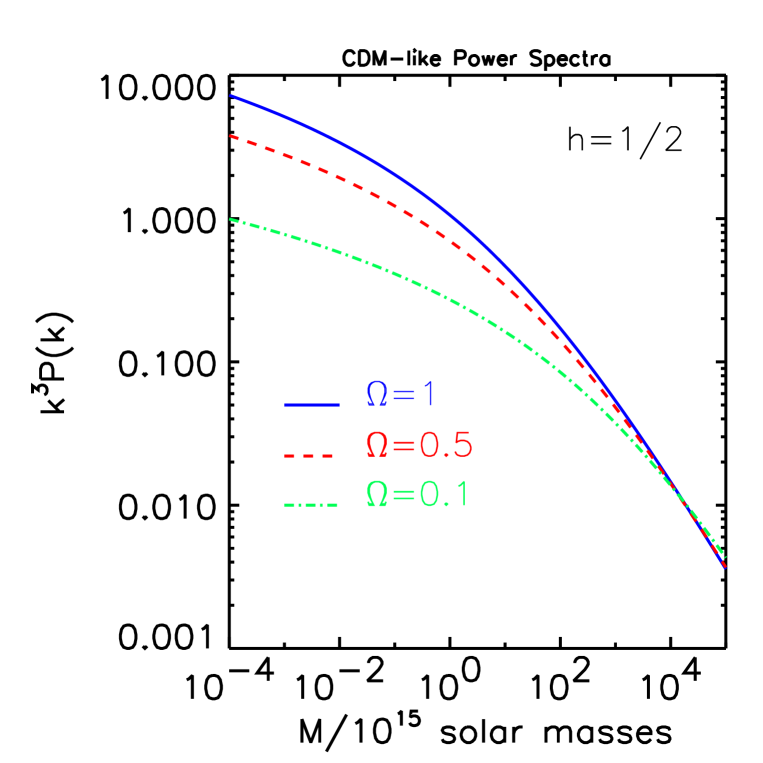
Figure 1: Cold dark matter density power spectra. The quantity $k^{3}P(k)$, approximately equal to the real–space density perturbation, is shown as a function of mass scale, $M=(4\pi/3)(2\pi/k)^{3}\rho_{b}$. All spectra have been arbitrarily normalized on large scales. The $x$–axis is given in units of $10^{15}\rm\,M_{\odot}$. The mass scale corresponding to the horizon at the radiation–matter transition is $\sim 10^{15}(\Omega h^{2})^{-2}\rm\,M_{\odot}$, or $1.0(\Omega h^{2})^{-2}$ in these units. From a power–law, all spectra gradually break over to a constant on small scales; the roll–over is very gradual. The spectra for the three different values of $\Omega$ demonstrate the effect of lowering the cosmic mean density, and thereby increasing the mass scale of the turnover.

4.3 Constructing the density power spectrum

To finally understand the general form of CDM–like power spectra using our previous results, we need to specify the primordial spectrum, say from Inflation. The simplest Inflation models are based on a quantum field in which no important physical scales are introduced (the fluctuating part of the quantum field is effectively free) – the only scale in the problem remains the proper (event) horizon $H^{-1}$ (a constant). During inflation, the proper wavelength of a quantum mode of the field grows exponentially with the expansion to eventually become much bigger than the horizon. When $a\lambda=H^{-1}$, we say the perturbation “crosses” the horizon, going out. It then becomes a classical perturbation mode subject only to gravitational influences. From what we have just said, we should not be surprised to learn that every perturbation looks the same as it crosses the horizon, because this is the only scale in the physics. In fact, the quantitative result we are looking for is that the density or gravitational potential perturbations crossing the horizon are fixed in real space; in terms of the power spectrum, this implies that $k^{3}P(k)=const$ at horizon crossing. Without too much extra complication, one can imagine a more general spectrum given by a featureless power–law: $k^{3}P(k)\propto k^{\gamma}$ at horizon crossing. This occurs, for example, in Inflation models where the energy density of the vacuum slowly decreases with time, resulting in a $\gamma<0$ (this does imply the introduction of an additional physical scale, namely the time constant for the vacuum evolution).

After Inflation, the horizon grows faster than the proper wavelength of a perturbation ($H^{-1}\sim t$ verses $a\lambda\sim a\sim t^{n}$, with $n<1$) and, one by one, the perturbations re-cross the horizon going in. Now, we have seen that in Poisson gauge super-horizon perturbations remain constant in the matter– and radiation–dominated epochs, i.e., $\dot{\psi}=\dot{\delta}=0$. If we ignore for simplicity their slight decay in the transition, we obtain that each perturbation re-enters with the same $k^{3}P(k)$ that it had going out. Perturbations therefore re–enter the horizon, at $\tau=\lambda$, with either increasing or decreasing amplitude, depending on the sign of $\gamma$. This implies that there must be a cut–off somewhere in the spectrum, because otherwise we would be faced with a hard divergence on either large or small scales. The special case of $\gamma=0$ avoids this (it has, in fact, a logarithmic divergence, which is much easier to treat) and leads to what is called a scale invariant spectrum, since each scale re–enters the horizon with the same amplitude. Because of its aesthetic properties, this scale invariant spectrum was postulated well before the concept of Inflation and is often referred to as the Harrison–Zel’dovich (HZ) spectrum. Remember that in the standard model, where only gravity plays a role, the evolution of perturbations may be studied independently of the exact mechanism responsible for their generation. One only needs to postulate an initial spectrum, such as a power–law. In these terms, Inflation is just one possible physical model attempting to explain the origin of the initial power spectrum. After this brief discussion, we shall no longer be concerned with the details of Inflation, and just adopt a power–law primordial spectrum.

Once inside the horizon, the perturbations evolve differently depending on the cosmic epoch, the various physical situations having been discussed in the previous two sections. Focus attention first on the cold dark matter (CDM), which is a cold collisionless fluid; hence, no pressure terms. The CDM perturbations remain constant after horizon crossing in the radiation–dominated epoch, and they only begin to grow, on all scales, after matter domination. This means that, for wavelengths smaller than the equality horizon, $k^{3}P(k)\propto k^{\gamma}$, or $P(k)\propto k^{-3+\gamma}$. On the other hand, a perturbation entering the horizon during the matter–dominated epoch begins to grow immediately. Horizon crossing occurs when $k=2\pi/\tau$, and because in the matter era $a\propto\tau^{2}$ and $P(k)\propto a^{2}$ (our perturbation result IA), we deduce that, on scales larger than the equality horizon, $P(k)\propto k^{1+\gamma}$. Now we change notation and define the spectral index as $n\equiv 1+\gamma$, so that at time $\tau$

$$P(k) \propto k^{n-4}\ \ \ \ \tau_{eq}<\tau<\lambda$$

$$P(k) \propto k^{n}\ \ \ \ \ \ \tau_{eq}<\lambda<\tau$$

$$P(k) \propto k^{n-4}\ \ \ \ \lambda<\tau_{eq}$$

where $\tau_{eq}$ refers to the comoving horizon at the matter–radiation transition (or the equality epoch). With $n=1$ the power–law on large scales is the more familiar form of the HZ spectrum, but its scale invariance is seen directly not in the power law, but in the behavior of each mode as it crosses the horizon.

Figure 1 shows several CDM–like power spectra, where we can see the features just described. There is the power–law decrease of $k^{3}P(k)$ towards large scales with the gradual break to a constant towards smaller scales. The spectra are plotted as a function of the mass enclosed in a sphere of radius $\lambda$. This permits us to easily identify galactic ($M\sim 10^{12}\rm\,M_{\odot}$) and cluster ($M\sim 10^{15}\rm\,M_{\odot}$) scales. In these terms, the scale at the break corresponds to the mass enclosed within the horizon at equality, namely $M_{eq}=10^{15}(\Omega h^{2})^{-2}\rm\,M_{\odot}$.

It is of fundamental importance that we have discovered a physical scale in the final power spectrum. This scale was not put in by hand; on the contrary, a featureless power–law was injected as an initial condition (the simplest general class imaginable). It is the subsequent evolution that has imposed this scale. This is extremely important, because we did not put in this scale to explain the galaxy distribution we observe today, but the fact is that this general form is exactly what is needed to explain both the COBE temperature perturbations (subject of the next section) and the overall amplitude of the galaxy fluctuations today. This is a remarkable fact that should not be lost on the reader. It is often remarked today that the COBE observations have killed the standard CDM model with $\Omega=1$, $h=0.5$, etc… The reason for this amounts to a factor of 2: once such a standard spectrum has been normalized on the largest scales by the COBE observations, the amplitude on galaxy cluster scales (many orders of magnitude below those of COBE) is too high by a factor of about 2. This is in fact enough to put the standard CDM model in jeopardy, but at a first look, one should be extremely impressed that the general form of $P(k)$ works so well over such a vast range of scales. The game today is to slightly change the matter density to fix this factor of 2. This works in part because the horizon scale at equality depends on the non–relativistic matter content of the Universe. Lower $\Omega$, with or without a cosmological constant, and you delay matter domination, increasing the scale of the break in $P(k)$. This is easily seen in Figure 1. The implications of a factor of 2 can be quite large - remarkable overall consistency, but in detail perhaps requiring a low density parameter. Not bad!

Most of the above discussion of the power spectrum concerns the evolution of the collisionless CDM. How about the baryons and photons? They behave as a single fluid dominated by the pressure of the photons before decoupling. As each perturbation in this fluid enters the horizon, it begins to oscillate as a sound wave, according to our perturbation solutions; this will become important when discussing the “Doppler” peaks of the temperature anisotropy power spectrum in the next section. It is only after decoupling, when the baryons are no longer hampered by pressure, that the perturbations can grow. Then, with the additional “pull” of the already growing CDM perturbations, the baryons eventually catch–up and develop a power spectrum similar to that of the dark matter. These perturbations then gradually collapse into dark halos containing baryons and form galaxies and galaxy clusters. The photons, on the other hand, just simply free–stream through space after decoupling, for the most part not interacting with anything else until the moment some of them are captured in one of our CMB experiments.

5 Temperature Anisotropies

The study of the evolution of density perturbations in the expanding Universe dates back to well before the prediction or discovery of the CMB. Lemaître himself was one of the first to propose that structure could be formed by such perturbations in his primeval atom picture. He also eagerly sought the relic radiation of the initial explosion, thinking that it was probably the cosmic rays. It was only much later, in 1948, that Gamow and his collaborators took things farther in suggesting that elemental abundances were established in the early Universe during a period of primordial nucleosynthesis dominated by thermal radiation. They predicted that this radiation should still be omnipresent today, with a temperature of about 5K. Not until quite a bit later was this radiation detected, and at first thought to be an unexpected noise signal, in Bell Laboratory’s Homdel telescope (Penzias & Wilson 1965; Dicke et al. 1965). Peebles (1993) and Partridge (1995) provide a history of the discovery of the CMB. Soon after this discovery and the associated rise to popularity of the Big Bang model, it was realized that the background radiation should carry the imprint of the density perturbations at early times in the form of temperature anisotropies (Sachs & Wolfe 1967; Peebles & Yu 1970). A new and powerful test of the Big Bang scenario was thus posed, and what was to become a much longer than expected search for these CMB anisotropies was begun, culminating finally in 1992 with their first detection by the COBE satellite (Smoot et al. 1992). Today, there are more than a dozen detections spanning many angular scales, as shown in Figure 3. For a good reference to the various experimental efforts in progress, see Smoot (1997).

In this chapter, we investigate the relationship between the density perturbations, studied at length in preceding section, and CMB anisotropies. Our ultimate goal is to explain the general features of the standard model anisotropies as presented, for example, by the curves in Figure 3. This is a subject rich in physical concepts; it may be as detailed and complicated as necessary to make predictions good to arbitrary accuracy, or as simple and naive as required to grasp only the essentials. In the following, we will search the middle ground, principally by developing ideas within the framework of a rather reasonable approximation known as the tight–coupling approximation. We shall once again only consider adiabatic perturbations.

To understand the nature of this approximation, recall the state of the Universe at the decoupling era, the surface we actually “see” in a map of the CMB (exactly what we observe will become more clear as we go along). At that time, the Universe consisted of a fluid with several components, namely baryons (mainly protons and Helium nuclei), free electrons, photons, neutrinos and, perhaps, a form of non–baryonic dark matter. Thomson and Coulomb scattering strongly coupled baryons, electrons and photons together, ensuring that they behave as a single fluid. This remained the case up til moments just before recombination, when the optical depth to scattering begins to become larger and larger. Recombination occurs when the majority of the ions have recombined, but actual decoupling of the photons, when their mean free path becomes larger than the particle horizon, occurs slightly afterwards. For standard recombination at redshifts near 1000, the transition from opacity to transparency is relatively rapid. The tight–coupling approximation describes decoupling and recombination as a single event, an infinitely rapid transition before which the baryon–photon fluid existed as a single entity and after which the baryons and photons are completely decoupled fluids; in other words, the surface of last scattering is imagined to be infinitely thin. In actuality, this is not too crude an approximation. The tight–coupling picture greatly simplifies the problem precisely because it permits us to treat the baryons and photons as a single fluid in the perturbation equations of the previous section. After decoupling, we again have a simple situation in which the photons simply free–stream away from the surface of last scattering.

Sufficiently armed with our tight–coupling approximation, we will seek to understand the general form of the standard model anisotropy power spectrum. We expect that Thompson scattering will be irrelevant on large angular scales (small $l$), that what we see reflects the initial photon perturbations and only purely kinematic gravitational effects, because all causal physics is unimportant. In fact, on these large scales, the tight–coupling concept serves no purpose; it is only on sub-horizon scales at decoupling that this concept has a useful meaning. The anisotropies on large scales can all be related to the gravitational field, and we call the relevant physics the Sachs–Wolfe (SW) effect. This is one of the two primary physical effects we need to understand in order to construct the power spectrum, and it will be treated in section 5.3. Although one often hears that the Sachs–Wolfe effect is only gravitational, the actual contribution to the observed anisotropies from the initial photon distribution and from gravitational redshift is gauge dependent, i.e., the individual contributions depend on the particular gauge chosen for the calculation. The final result is all the same gauge invariant, because it is what we actually observe. On angular scales below the decoupling horizon (large $l$), casual physics, i.e., pressure effects, will govern the evolution of the perturbations, and hence the production of anisotropies. This is the other key physical effect we need to construct the power spectrum, and it is treated first, in section 5.2. In the tight–coupling limit, the photons and baryons act as a fluid with large pressure, and we have seen that sub–horizon perturbations in such a fluid become sound waves. We expect to see their signature in the CMB anisotropies on smaller angular scales; they produce the famous “Doppler peaks” predicted around degree angular scales, demonstrated by the curves in Figure 3.

We saw before how the horizon size at the matter–radiation transition became the only important scale characterizing the final density perturbation power spectrum. From this discussion, we should expect to find that the angular size of the horizon at decoupling ($\sim 0^{o}.5$ $\Omega^{1/2}$) will impose itself as a founding scale in the CMB anisotropy power spectrum. This is an important point; it will, among other things, offer us a way to constrain the global geometry of the Universe.

5.1 Describing the CMB sky

Before we can dive into calculations of CMB anisotropies, we must decide what to calculate. This depends on the quantities used to describe the anisotropies. Just as for the density field, we describe the CMB sky as a random field, in two dimensions: $\Delta(\hat{n})\equiv\delta T(\hat{n})/T$, where $\hat{n}$ is a unit vector on the sphere. This means that the value of $\Delta$ at each position on the sphere (sky) is a random variable. By definition $<\Delta(\hat{n})>=0$, and the two–point (auto–) correlation function gives the covariance of these random variables as

$$C(\theta)=<\Delta(\hat{n}_{1})\Delta(\hat{n}_{2})>$$

with $\cos\theta=\hat{n}_{1}\cdot\hat{n}_{2}$. Notice that the correlation function only depends on the separation of the two sky directions, $\theta$. This is once again the work of the cosmological principle: the nature of the anisotropies must be independent of position or orientation on the sky. This is a statement that the temperature fluctuations were generated by a statistically isotropic and homogeneous process. Because the mean of $\Delta$ is by construction zero, Gaussian anisotropies, as in the standard model, are completely specified by the two–point correlation function.

It once again proves convenient to work with the harmonic modes of our random field. On the sphere we employ the spherical harmonic transform:

$$\Delta(\hat{n})=\sum_{lm}a_{lm}Y_{lm}(\hat{n})$$

The coefficients $a_{lm}$ are random variables with $<a_{lm}>=0$. We should expect, as before for the density field, that their covariance is related to the two–point correlation function. To find this covariance, first note that since the two–point correlation function only depends on separation, we may expand it in a Legendre series

$$C(\theta) = \frac{1}{4\pi}\sum_{l}(2l+1)C_{l}P_{l}(\hat{n}_{1}\cdot\hat{n}_{2})$$ (50)

$$= \sum_{lm}C_{l}Y_{lm}(\hat{n}_{1})Y^{*}_{lm}(\hat{n}_{2})$$ (51)

where we have used the addition theorem of spherical harmonics to get to the second line. This permits us to easily calculate the quantity

$$<a_{lm}a^{*}_{l^{\prime}m^{\prime}}> = \int\int d\Omega_{1}d\Omega_{2}\;<\Delta(\hat{n}_{1})\Delta(\hat{n}_{2})>Y^{*}_{lm}(\hat{n}_{1})Y_{l^{\prime}m^{\prime}}(\hat{n}_{2})$$

$$= \int\int d\Omega_{1}d\Omega_{2}\;C(\theta)Y^{*}_{lm}(\hat{n}_{1})Y_{l^{\prime}m^{\prime}}(\hat{n}_{2})$$

with the important result

$$<a_{lm}a^{*}_{l^{\prime}m^{\prime}}>=C_{l}\delta_{ll^{\prime}}\delta_{mm^{\prime}}$$ (52)

The presence of the $\delta$ functions tells us that the $a_{lm}$ are independent random variables. This is a direct consequence of the fact that the two–point correlation function only depends on separation, i.e., the cosmological principle. The set of $C_{l}$ is the (angular) power spectrum of the temperature anisotropies, and for the Gaussian fluctuations encountered in the standard model, it is a complete description of the CMB sky, just as the density power spectrum is a complete description of the density field in Gaussian models. The angular power spectrum is thus the fundamental quantity in the theory of CMB anisotropies of the standard model. Non–Gaussian theories would require consideration of higher order moments of the field $\Delta$.

Our goal is now clearly before us: to find the $C_{l}$ and their relation to $P(k)$ of the density field. Specifically, we wish to construct and understand the overall form of the angular power spectrum of the standard model anisotropies, as for example presented in Figure 3. This work is the analog of our efforts to understand the general form of the density field as described by $P(k)$.

5.2 Start with the simple

So, just how do the density perturbations leave their imprint on the photons? We proceed by first ignoring various effects, to be re–added later. Suppose, then, that in addition to our basic assumption that the surface of last scattering is infinitely thin, space is flat and static (no curvature, no expansion) and completely uniform and homogeneous after decoupling. This means in particular that, although there are perturbations on the last scattering surface, they do not exist between us and this surface, and that there are no important photon interactions off the surface of last scattering; this is all, of course, highly unrealistic, but we will remedy that as we go along. We solve this problem, a standard problem of classical physics, in this subsection. This will give us some understanding of how we directly “see” the photon perturbations on the last scattering surface. The intuition we gain in this manner will in practice only apply to small angular scales. To go beyond this, we will need to introduce some important concepts of photon transport in GR, presented in the following subsection. These will permit us to add back into the problem the expansion and curvature of space, as well as perturbations after decoupling. It is here that we encounter the famous Sachs–Wolfe (SW) effect, which dominates the CMB anisotropies on large angular scales.

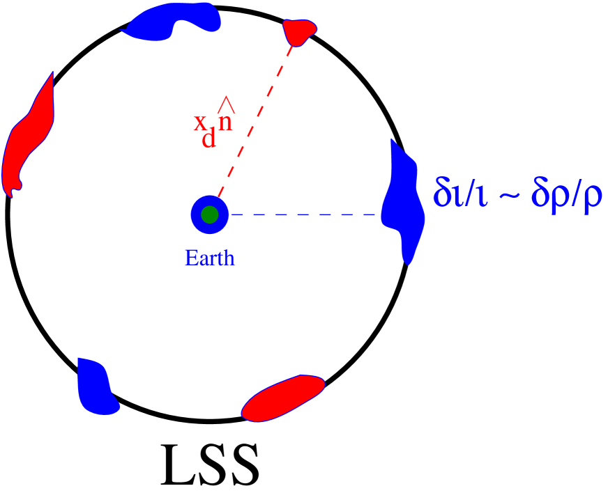
Figure 2: Schematic diagram of the last scattering surface. The observer is at the center and sees the fluctuations on the last scattering surface at a distance of $x_{d}\hat{n}$. In the tight–coupling approximation, the photon intensity perturbations on the surface, $\delta{\iota}/{\iota}$, are equal to the photon density perturbations, $\delta\rho_{\gamma}/\rho_{\gamma}$. On sub–horizon scales, the baryon–photon fluid oscillates with sound waves, which are then seen by the observer as peaks and valleys in the $C_{l}$ verses $l$ plane (Eq. 59).

We have before us a straightforward problem of classical physics: how to describe the intensity pattern on a distant screen (see Figure 2). More precisely, we place ourselves at the origin of a sphere and the screen corresponds to the inside surface of this sphere at a distance of $x_{d}$ (the distance to the last scattering surface). Suppose that the intensity pattern on the screen is given by ${\iota}(\hat{n},t_{d})$, where $t_{d}$ is the time at decoupling, when the light is emitted from the screen. The intensity that we measure today, at time $t_{o}$ sitting at the origin of our coordinate system ($\vec{x}=0$), and coming from direction $\hat{n}$, is ${\iota}(-\hat{n},t_{o},\vec{0})={\iota}(-\hat{n},t_{d},x_{d}\hat{n})$, because surface brightness is conserved (remember, we are ignoring expansion for the time being). In the tight–coupling limit, the radiation intensity at decoupling may be written in terms of the photon energy density, $\rho_{\gamma}$, as ${\iota}=(c/4\pi)\rho_{\gamma}$. Notice that this means that the photon intensity at an arbitrary point in the baryon–photon fluid is independent of propagation direction; this is a direct consequence of the tight–coupling assumption, and the breakdown of this exact condition is one of the complications to be treated in a more complete calculation. Thus, we have arrived at the statement

$$\Delta \equiv \frac{\delta{\iota}}{{\iota}}(-\hat{n},to,\vec{0})=\delta_{\gamma}(x_{d}\hat{n},t_{d})$$ (53)

$$= \frac{1}{(2\pi)^{3}}\int d^{3}k\;e^{-ix_{d}\hat{n}\cdot\vec{k}}\delta_{\gamma}(\vec{k},t_{d})$$ (54)

In the last line we have expressed the photon perturbation in terms of its Fourier transform, the kind of quantity we used when discussing density perturbations previously. Using an identity which translates basis functions from Cartesian coordinates to spherical coordinates,

$$e^{-i\vec{k}\cdot\vec{x}}=4\pi\sum_{lm}\;(-i)^{l}j_{l}(kx)Y^{*}_{lm}(\hat{k})Y_{lm}(\hat{x})$$ (55)

we can write the observed intensity perturbation today as

$$\Delta(\hat{n})=\sum_{lm}\;\left[4\pi(-i)^{l}\frac{1}{(2\pi)^{3}}\int d^{3}k\;j_{l}(kx_{d})Y^{*}_{lm}(\hat{k})\delta_{\gamma}(\vec{k},t_{d})\right]Y_{lm}(\hat{n})$$ (56)

from which we learn that the $a_{lm}$ are given by the expression in square brackets; this is the sought relation between the perturbations and the $a_{lm}$ describing the observed anisotropies of the CMB. Not so difficult in the end!

It is clear from the linear nature of this relationship that the $a_{lm}$ retain all the statistical properties of the perturbation variables; if these latter are Gaussian random variables, as in the case of inflationary models, then so are the spherical harmonic coefficients. We can be more quantitative. It is easy to see that $<a_{lm}>=0$, which is no surprise. As for the covariance of the harmonic coefficients, this is calculated as follows:

$$<a_{lm}a^{*}_{l^{\prime}m^{\prime}}> = \frac{1}{4\pi^{4}}(-i)^{l}(+i)^{l^{\prime}}\int d^{3}k\;d^{3}k^{\prime}j_{l}(kx_{d})j_{l}(k^{\prime}x_{d})$$ (58)

$$Y^{*}_{lm}(\hat{k})Y_{l^{\prime}m^{\prime}}(\hat{k}^{\prime})<\delta_{\gamma}(\vec{k},t_{d})\delta_{\gamma}(\vec{k}^{\prime},t_{d})>$$

By using Eq. (12) and recalling that $<a_{lm}a^{*}_{l^{\prime}m^{\prime}}>=C_{l}\delta_{ll^{\prime}}\delta_{mm^{\prime}}$, we find an expression for the $C_{l}$:

$$C_{l}=\frac{2}{\pi}\int dk\;k^{2}P_{\gamma}(k)j^{2}_{l}(kx_{d})$$ (59)

Within the limits of our simplifying assumptions, which we will now gradually relax, this is a central relation between CMB anisotropies and density perturbations at the epoch of last scattering. If the latter are calculated using perturbation theory, and note that here we specifically need the photon perturbation, $\delta_{\gamma}$, then we can find the $C_{l}$ that an observer would deduce. In the tight–coupling approximation, $\delta_{\gamma}$ is easily calculated from the evolution of the baryon–photon fluid. Corrections to the this approximation render things more complicated precisely because we are saying that the two components do not behave in exactly the same manner. It is here that one must start to employ the Boltzmann equation to perform an accurate calculation.

We have achieved one of our goals, that of describing the the relationship between the density perturbations and the anisotropies on small scales. In the tight–coupling limit, the baryon–photon fluid is oscillating on the last scattering surface, creating the Doppler peaks seen in the $C_{l}$. We have indeed made many assumptions to arrive at this result, but the important point is that the essence of the physics of the problem is revealed without excessive detail (to be added at will!); and the line of reasoning leading to these results will be reused in the following.

5.3 A traveling photon

We wish to relax the simplifying restrictions employed in the last subsection. Among other things, we are now forced to consider more carefully just exactly how a photon travels between us and the last scattering surface. This is a must if we wish to understand the influence of perturbations after decoupling. Consider a packet of photons, or light ray, following a trajectory $x^{\alpha}(\lambda)$ in spacetime and described by four momentum $p^{\alpha}(\lambda)$. The affine parameter $\lambda$ labels position along the photon path. Photons are zero mass particles, so they travel along null geodesics:

$$\frac{dp^{\alpha}}{d\lambda} + \Gamma^{\alpha}_{\beta\gamma}p^{\beta}p^{\gamma}=0$$

$$p^{\alpha}\equiv\frac{dx^{\alpha}}{d\lambda}$$

$$p^{2}=0$$

The affine parameter is defined by the second equation; the third specifies that the path is a null geodesic. We already see from this basic equation how gravity influences the CMB – via the Christoffel symbols characterizing the spacetime geodesics. This is in fact the equation we will employ to find $\delta T/T$, thanks to the fact that Gravity is color blind; however, it is useful to at least see a little of the Boltzmann equation, which is used in more complete calculations of temperature anisotropies.

Evolution of the photon “gas” can be modeled by its phase space distribution function, $f(x^{\alpha},p^{i})$, and we assume that this gives a complete description of the CMB (no higher order correlations or collective effects in the gas). It is important to notice that $f$ here is taken to be a function of the contravariant four–position and of the contravariant three–momentum. This is not obvious, because it is in fact the covariant three–momentum which is the dynamically conjugate variable to position, but the isomorphism between covariant and contravariant vectors ($p^{\alpha}=g^{\alpha\beta}p_{\beta}$) permits us to do this. Since we will be primarily interested in the free streaming of CMB photons after scatterings have ceased to be important (tight coupling means that we can forget about photon transport before decoupling, treating everything as a simple fluid), we employ the Liouville equation (Boltzmann equation with no sources)

$$\frac{Df}{D\lambda}=p^{0}\frac{\partial f}{\partial x^{0}}+p^{i}\frac{\partial f}{\partial x^{i}}+\frac{dp^{i}}{d\lambda}\frac{\partial f}{\partial p^{i}}=0$$

Gravity enters here through the geodesic equation describing the photon path, Eq. (5.3).

How is this equation actually used? The first thing one must do in a general situation is to find the form of the null geodesics, $x^{\alpha}(\lambda)$ and $p^{\alpha}(\lambda)$, given a coordinate system [Christoffel symbols $\Gamma^{\alpha}_{\beta\gamma}(\lambda)$]. These quantities are then plugged into the Liouville equation, which one can now integrate to find the solution $f[x^{\alpha}(\lambda),p^{i}(\lambda)]$. We do this, as an illustration, for the perfectly homogeneous and flat FRW background. This is only for illustration; as mentioned, in our discussion on perturbations we shall in fact get by with only the geodesic equation. The Christoffel symbols in conformal coordinates ($\tau,\vec{x}$) are given by Eqs. (28)–(33), with all perturbation variables set to zero. With flat space–like slices, we know that all geodesics are “normal” straight lines, i.e., we can describe them by $x^{1}(\lambda)=x^{0}(\lambda)=\tau(\lambda)$, $x^{2}=x^{3}=0$ and $p^{1}=p^{0}\equiv p(\lambda)$, $p^{2}=p^{3}=0$ (notice that $p^{2}=0$ as required). The zero component of the geodesic equation then yields $p\propto 1/a^{2}$, which you find very upsetting, because everybody knows that the redshift is $\propto 1/a$. So what happened?! Everything is in fact OK, because this momentum is the conjugate variable to $\tau$, i.e., $p=d\tau/d\lambda$; the conjugate variable to cosmic (local observer) time $t$, let’s call it $q$, is related via $q=dt/d\lambda=(d\tau/d\lambda)(dt/d\tau)=ap\propto 1/a$, and we are reassured. Moral: let’s not forget that we are manipulating conformal time in the following. The space components of the geodesic equation simply confirm the fact that $p^{1}=p^{0}=p$ and $p^{2}=p^{3}=0$ all along the trajectory, that our choice is consistent.

Now put these results into the Liouville equation to find

$$p\frac{\partial f}{\partial\tau}+p\frac{\partial f}{\partial x^{1}}+\frac{dp}{d\lambda}\frac{\partial f}{\partial p}=0$$

or

$$\frac{\partial f}{\partial\tau}+\frac{\partial f}{\partial x^{1}}-2\frac{\dot{a}}{a}p\frac{\partial f}{\partial p}=0$$

In our perfectly uniform background, we also know that $f$ does not depend explicitly on position, $x^{i}$, so we are left with a very simple expression:

$$\frac{\partial f}{\partial\tau}-2\frac{\dot{a}}{a}p\frac{\partial f}{\partial p}=0$$

whose solution is $f(\tau,p)=f(\tau_{i},pa^{2}/a_{i}^{2})$, where $\tau_{i}$ is some initial time at which the phase function is given (this is enough, because the Liouville equation is first order).

Suppose that at some initial time (in a space–like slice at constant $t$ or $\tau$) all comoving observers see the Universe filled with blackbody radiation. Everyone thus remarks that $f=(e^{\omega/T}-1)^{-1}$, where $\omega$ is the observed frequency, or energy, as measured by a comoving observer. We must be very careful to correctly interpret our momentum variable in terms of this observed energy, the main difficulty being that we are working in a gauge where $g_{00}\neq 1$. In general, the energy measured by an observer with 4–velocity $u^{\alpha}$ is given by the covariant expression $\omega=p^{\alpha}u_{\alpha}$. Using the condition $u^{\alpha}u_{\alpha}=g_{\alpha\beta}u^{\alpha}u^{\beta}=1$ and noting that comoving observers have $u^{i}=0$, we see that $u^{0}=g_{00}^{-1/2}$; hence, $\omega=g_{00}p^{0}u^{0}=g_{00}^{1/2}p^{0}=ap$, and not simply $p^{0}$. Thus, $f(\tau_{i},p)=(e^{a_{i}p/T}-1)^{-1}\equiv B(a_{i}p/T)$, and this is the same for everybody. Our result is that at later times $f(\tau,p)=B[a^{2}p/(a_{i}T)]=B[\omega/(a_{i}T/a)]$, from which one concludes that the spectrum is still thermal, but now with a temperature $Ta_{i}/a$. This is the familiar redshift law for the CMB temperature. The result is immediately obvious from the geodesic equation, which tells us that all photons experience the same redshift, but this derivation helps to understand the workings of the Liouville equation.

Let’s now turn our attention to the effects of metric perturbations on the CMB. Fortunately, gravity is color blind, meaning that it does the same thing to photons of any frequency (this is a consequence of the equivalence principle). Thus, metric perturbations will not alter the thermal nature of the CMB frequency spectrum. For this reason, we can get quite far in our analysis by only using the geodesic equation for the photons; whatever happens to one set of photons happens to all of them following a particular path, and so this evolution must therefore also be the same as the temperature of the thermal spectrum. We choose to work in Poisson gauge and, to keep things as simple as possible, with a flat space background. Only scalar perturbations in an ideal fluid will be considered, so the only relevant metric perturbation variable is the “Newtonian” potential, $\psi$. The technique is to expand the geodesic equation (5.3) out to first order in the perturbation variables. Our primary concern is with the time component

$$\frac{dp^{0}}{d\tau}=-\frac{\dot{a}}{a}\left(p^{0}+\gamma_{ij}p^{i}\frac{p^{j}}{p^{0}}\right)+\dot{\psi}\left(\gamma_{ij}p^{i}\frac{p^{j}}{p^{0}}-p^{0}\right)+4\frac{\dot{a}}{a}\gamma_{ij}\frac{p^{i}p^{j}}{p^{0}}\psi-2p^{i}\psi_{,i}$$ (61)

Notice that the original derivative with respect to $\lambda$ has been converted to a derivative with respect to $\tau$ (by dividing through by $p^{0}$). Imposed on this equation is the condition $p^{2}=0$:

$$(1+2\psi)(p^{0})^{2}-(1-2\psi)\gamma_{ij}p^{i}p^{j}=0$$ (62)

from which we immediately learn that the expression in parenthesis in the second term of Eq. (61) is first order, and hence the whole second term may be dropped. By defining $p\equiv\sqrt{\gamma_{ij}p^{i}p^{j}}$, we put Eq. (62) into the compact form

$$p^{0}=(1-2\psi)p$$

We may then also write $p^{i}=pn^{i}$, where the $n^{i}$ are the direction cosines along the photon path such that $\gamma_{ij}n^{i}n^{j}=1$. To first order, this reduces the geodesic equation to

$$\frac{1}{a^{2}p^{0}}\frac{d}{d\tau}(a^{2}p^{0})=-2n^{i}\psi_{,i}$$

where we have used the fact that $dx^{i}/d\tau=p^{i}/p^{0}$ is equal to $n^{i}$ to zero order, as appropriate to keep the final expression to first order.

We now use some of our previous results concerning the evolution of the gravitational potential, $\psi$. In the matter–dominated era, when $x\sim c_{s}^{2}\sim 0$, we have seen that $\dot{\psi}=0$ for modes outside the horizon, $\lambda>\tau$. The same holds for sub–horizon perturbations when the curvature/cosmological constant terms are unimportant, i.e., at all times in a critical model or at sufficiently early times in non–critical models. This is most easily seen from our Newtonian result that $\delta_{g}\propto a$; hence, the Poisson equation tells us that $\phi_{k}\propto\rho_{b}a^{2}\delta_{g}=const$ (matter–dominated epoch). For the following calculation, we shall in practice adopt the critical model and ignore any possible residual effects of the radiation–matter transition at the moment of last scattering; we will make some brief comments below concerning modifications in non–critical models (in passing, we note that even in flat models ($\Lambda\neq 0$) the radiation–matter transition approaches the last scattering surface as $\Omega$ is lowered). Then, we may write

$$\frac{d\psi}{d\tau}=\dot{\psi}+n^{i}\psi_{,i}=n^{i}\psi_{,i}$$

leading to our final result

$$\frac{1}{a^{2}p^{0}}\frac{d}{d\tau}(a^{2}p^{0})=-2\frac{d\psi}{d\tau}$$ (63)

Apart from factors of $a$, this is the traditional result for the gravitational redshift due to a potential $\psi$; and no, the factor of 2 is not a typo! The rational for this factor of 2 provides a good exercise in understanding measurements in GR. Key question in all situations: what are we trying to calculate, or what is the measurement that interests us? We really want to find the frequency (energy) shift as measured by two observers, one at each end of the photon path and each at rest relative to the coordinate system. As already mentioned, the fact that we are working in a gauge (coordinate system) where $g_{00}\neq 1$ means that we must use extreme care in interpreting $p^{0}$. We have two observers, one at the emission point, $x_{e}$, and the other at the reception point, $x_{r}$. Since each is at rest relative to the coordinate frame in use, each one has a four–velocity with zero spatial components. From the requirement that $u^{\alpha}u_{\alpha}=1$, we find, as before, that $u^{0}=g_{00}^{-1/2}$. This time, working to first order, we thus obtain the measured frequency at each point $\omega=g_{00}p^{0}u^{0}=a(1+\psi)p^{0}$. Consider first the classic case encountered in most textbooks, i.e., $a=1$, a constant which may be dropped from our expressions. To first order, the geodesic equation then yields a frequency shift of

$$\frac{\Delta\omega}{\omega}=-2\Delta\psi+\Delta\psi=-\Delta\psi$$

a reassuring and familiar expression.

How about when $a$ is not constant, as in our cosmological setting? Let us again be very careful and explicit about what it is we should calculate in our perturbation theory. We want the temperature perturbation induced by $\psi$, relative to the unperturbed background model. In the background model (pure FRW), we know that $a\omega=const$, i.e., $\Delta(a\omega)=0$. Thus we should find $\Delta(a\omega)/(a\omega)$ – this is the $\delta T/T$ that we seek. Because the numerator of this ratio is of first order, the denominator is left to order zero – a constant – and so may be specified at either end of the photon path. In the following expression, $r$ and $e$ refer to the points of reception and emission, respectively:

$$\frac{\delta T}{T} = \frac{\Delta(a\omega)}{a\omega}$$

$$= \frac{a_{r}^{2}[1+\psi(r)]p^{0}(r)-a_{e}^{2}[1+\psi(e)]p^{0}(e)}{a^{2}p^{0}}$$

$$= \frac{\Delta(a^{2}p^{0})+a^{2}p^{0}\Delta\psi}{a^{2}p^{0}}$$

$$= -\Delta\psi$$

where we have used Eq. (63) to get to the last line. From the second to the third, we used the fact that $a^{2}p^{0}=const$ to zero order. The beauty of the result is that it is exactly what we would have guessed, given the concept that $\psi$ is a kind of Newtonian potential.

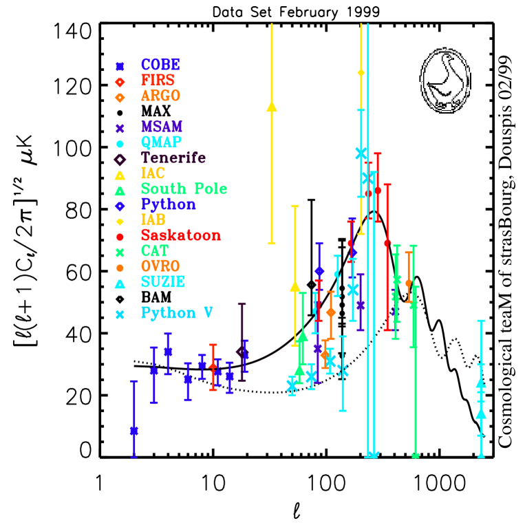
Figure 3: Angular power spectrum of the CMB anisotropies. The data come from the various experiments as indicated by the color code on the left. The solid curve is the prediction for a flat CDM model with $\Omega=0.4$, $\Lambda=0.6$, $H_{o}=40$ km/s/Mpc, $Q=19\;\mu$K, $\Omega_{b}h^{2}=0.006$ and $n=0.94$, while the dotted line represents an open model with $\Omega=0.2$, $\Lambda=0$, $H_{o}=60$ km/s/Mpc, $Q=20\;\mu$K, $\Omega_{b}h^{2}=0.015$ and $n=1$ (no gravitational waves, no reionization). Late–time evolution of the gravitational potential in the flat model is not important enough to alter the basic result expressed in Eq. (66) for $n=1$ – we see a plateau in $l(l+1)C_{l}$. In the open model, on the other hand, late–time evolution of $\psi$ is sufficiently important to substantially modify the plateau. The Doppler peaks at higher $l$ are the projected acoustic oscillations of the baryon–photon fluid on the last scattering surface, Eq. (59). Curvature in the open model has shifted the angular position of the first peak to higher $l$ compared to the flat scenario. Figure prepared by M. Douspis; see http://astro.u-strasbg.fr/Obs/COSMO/CMB/

To get the classical SW expression, we need now to consider the initial conditions corresponding to adiabatic perturbations. Since the relative particle densities remain constant in this kind of perturbation, we may relate the dominate (non–relativistic) dark matter perturbation to the CMB temperature perturbation by $\delta\propto 3\delta T/T$. For super-horizon perturbations ($\dot{\psi}=0$) on the last scattering surface (i.e., on angular scales larger than $\sim 0^{o}.5$), our perturbation Eq. (49) tells us that, in the initial hyper-surface, $\delta T/T(e)=(1/3)\delta(e)=-(2/3)\psi(e)$. We remark in passing that in our perturbation theory the initial hyper-surface is defined by $\tau=const$; and this implies that, to first order, $\psi(e)$ is to be taken in the surface defined to zero order, which is the same surface as in the background. This leads to

$$\frac{\delta T}{T}=-\Delta\psi+\frac{\delta T(e)}{T}=-\psi(r)+\frac{1}{3}\psi(e)$$

Since $\psi(r)$ is a constant independent of direction on the sky, and what we measure is a difference between different directions, our answer is the well known result

$$\frac{\delta T}{T}=\frac{1}{3}\psi(e)$$ (64)

which was the remaining goal we had set before us at the beginning of this chapter.

To finally get to the $C_{l}$ plot, we need to translate the SW relation (64) into $C_{l}$. Remember, the SW effect dominates the temperature fluctuations on large angular scales, which means at small $l$. Using the same reasoning as before, in going from Eq. (54) to Eq. (59), we obtain

$$C_{l}=\frac{2}{3\pi}\int dk\;k^{2}P_{\psi}(k)j_{l}^{2}(kx_{d})$$ (65)

where $<\psi_{\vec{k}}\psi^{*}_{\vec{k^{\prime}}}>=(2\pi)^{3}P_{\psi}(k)\delta(\vec{k}-\vec{k^{\prime}})$ defines the gravitational potential power spectrum. Recalling that on super-horizon scales $P_{\psi}(k)\propto k^{n-4}$, we see that

$$C_{l}^{SW} \propto \int dk\;k^{n-2}j^{2}_{l}(kx_{d})$$ (66)

$$\propto \frac{\Gamma(3-n)\Gamma\left(\frac{n+2l-1}{2}\right)}{\Gamma^{2}\left(\frac{4-n}{2}\right)\Gamma\left(\frac{5+2l-n}{2}\right)}$$

$$\propto \frac{1}{l(l+1)}\ \ \ \ \ \ \ \ \ \ \ \ \ (n=1)$$

Note that the last expression is only valid for the HZ spectrum, $n=1$. Two examples of CMB angular power spectra are shown in Figure 3 superimposed on the current data set. The flat model (solid curve) displays characteristics very similar to those of a purely critical model; in particular, as $n\sim 1$ in this model, we see the flat SW plateau expected according to Eq. (66).

The critical element in this derivation was the constancy of the gravitational potential $\psi$ along the photon path, something which breaks down when the Universe is not completely matter dominated. This occurs, for example, at late times in non–critical models and on the last scattering surface if $\Omega$ is low, because the radiation–matter transition is moved closer to this surface. An evolving $\psi$ creates an additional effect often refered to as the integrated Sachs–Wolfe (ISW) effect. This occurs because a photon does not climb out of the same potential well as it fell into, due to the evolution of $\psi$. This adds to the anisotropy calculated above and can significantly change the shape of the spectrum, most markedly at low $l$. We see this for the open model shown in Figure 3: even though the primordial spectrum has $n=1$, a flat SW plateau no longer exists. In the flat model shown, the ISW effect is small enough that we still clearly see a flat SW plateau similar to that expected from a purely critical model with $n=1$. We shall not go into further detail on this subject.

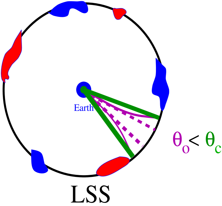
Figure 4: Same as Figure 2, but showing null geodesics in a flat (straight, green lines) and an open (negative curvature) Universe (curved, red lines). The curving geodesics in the open model project back onto the surface of last scattering (dashed, red lines) with a smaller angle than for the straight geodesics. The focusing of light rays in a curved Universe thus reduces the angular size subtended by the horizon at last scattering in the open model, $\theta_{o}$, compared to the critical model, $\theta_{c}$.

5.4 Constructing the anisotropy power spectrum

We have now in hand the two main results needed to understand the overall form of the anisotropy power spectrum: on large scales, those larger than the horizon at decoupling, it is the SW effect which is responsible for the temperature fluctuations, Eq. (66), while on scales below this horizon, we observe the acoustic oscillations via the relation (59); additional anisotropy sources exist in non–critical models, such as the ISW effect. Spectrum plots, such as the one shown in Figure 3, are made with $l(l+1)C_{l}$, so that a scale invariant HZ spectrum (in a critical Universe) appears as a horizontal line at low $l$. Once again, the horizon is the scale imposed on the problem. For standard recombination at $z\sim 1000$, the projected angular size of the horizon at last scattering is $\sim 0^{o}.5\Omega^{+1/2}$ (assuming a zero cosmological constant). This angular scale represents a transition from the large–scale behavior, e.g., the flat SW spectrum of Eq. (66) in critical models, to the oscillations of Eq. (59), which are seen as the famous “Doppler” peaks in the anisotropy power spectrum. We have thus accomplished our task of explaining the overall form of plots such as Figure 3.

We have not discussed the ISW effect and its consequences in any detail, nor shall we. Another consideration which we only touch on now in passing concerns the effect and spatial curvature. This is extremely important, because it determines the angular size subtended by the decoupling horizon, as diagramed in Figure 4. The focusing of light rays in a negatively curved Universe means that the projected angular size of the horizon at decoupling, as seen by us today, is smaller than for a critical Universe. The position of the first Doppler peak thereby offers a measure of the curvature of the Universe: in a model with large curvature, we expect the first peak to appear at higher $l$ than in a critical Universe, as shown by the dotted curve in Figure 3. These remarks in fact only apply to adiabatic perturbations; the location of the first peak is slightly different for isocurvature perturbations. As our goal is not to expose all possible effects and their dependence on the various cosmological parameters, we shall end our discussion here, content with our rapidly acquired understanding of the general form of the angular power spectrum.

6 Conclusion

The aim of these lectures has been to understand the physics responsible for the overall properties of the standard model density and temperature anisotropy power spectra (Figures 1 and 3). Perturbations in the standard model are taken to be Gaussian, and so these two quantities are the fundamental and unique characterization of the perturbations. An extremely significant point is that the physics governing perturbation evolution has imposed important scales on these power spectra. These scales were not present in the primordial spectrum, which we took to be a pure power–law. For the density perturbations, the imposed scale corresponds to the comoving horizon at the radiation–matter transition (the equality epoch). The final density power spectrum, thanks to this imposed scale, has roughly the correct shape to explain both the observed large–scale CMB fluctuations and the measured galaxy distribution today. This is a remarkable concordance over many orders of magnitude, a true success for the basic theory. In detail, the favored critical CDM model fails by a factor of two over this vast range; other models with a lower product of $\Omega h$ are perfectly compatible with the present data.

The scale imposed on the angular power spectrum of the CMB anisotropies is the projected size of the horizon at recombination. The Doppler peaks should first appear on this angular scale, and because the projected angle depends on the curvature of space (e.g., Figure 4), we have in principle a way to measure this fundamental quantity. Our discussion has focussed only on adiabatic perturbations, ignoring the possibility of isocurvature modes. The position of the first Doppler peak is not exactly the same for these latter, but the basic principles governing its location are. In fact, the fine details of the Doppler peaks depend on virtually all cosmological parameters, leading to the hope that we may measure them with precision observations of the CMB; this has become a preponderant subject of current cosmological research. It is important to remark that this en-devour will depend on the nature of the underlying model: cosmic defect models certainly do not predict the same dependence on cosmological parameters as the standard model we have considered. The CMB data will, of course, also tell us which type of model is correct (at present, it appears that defect models have difficulty in explaining the CMB anisotropies and the density power spectrum). At any rate, our brief discussion here is but an introduction to an ever-growing subject which will take a center stage role in cosmology for the coming years.

Acknowledgments

I would like thank the organizers and staff for a very enjoyable school, and the students for their hard work. Many thanks R. Durrer for discussions of a factor of 2 over the course of two years! I also thank M. Douspis for his very nice anisotropy power spectrum plot.

General references are given in the Introduction.

References

- [1] Dicke R.H., Peebles P.J.E., Rolls P.G., Wilkinson D.T. 1965, ApJ 142, 414
- [2] Partridge R.B. 1995, 3K: The Cosmic Microwave Background Radiation, Cambridge Astrophysics Series, Cambridge University Press (Cambridge)
- [3] Peebles P.J.E. & Yu J.T. 1970, ApJ 162, 815
- [4] Penzias A.A. & Wilson R.W. 1965, ApJ 142, 419
- [5] Sachs R.K. & Wolfe A.M. 1967, ApJ 147, 73
- [6] Smoot G.F. 1997, astro–ph/9705135
- [7] Smoot G.F. et al. 1992, ApJ 396, L1