Nature of Clustering in the Las Campanas Redshift Survey

Abstract

We have carried out a multi-fractal analysis of the distribution of galaxies in the three Northern slices of the Las Campanas Redshift Survey. Our method takes into account the selection effects and the complicated geometry of the survey. In this analysis we have studied the scaling properties of the distribution of galaxies on length scales from $20h^{-1}{\rm Mpc}$ to $200h^{-1}{\rm Mpc}$. Our main results are: (1) The distribution of galaxies exhibits a multi-fractal scaling behaviour over the scales $20h^{-1}{\rm Mpc}$ to $80h^{-1}{\rm Mpc}$, and, (2) the distribution is homogeneous on the scales $80h^{-1}{\rm Mpc}$ to $200h^{-1}{\rm Mpc}$. We conclude that the universe is homogeneous at large scales and the transition to homogeneity occurs somewhere in the range $80h^{-1}{\rm Mpc}$ to $100h^{-1}{\rm Mpc}$.

1 Introduction

Many surveys have been carried out to chart the positions of galaxies in large regions of the universe around us, and many more surveys which go deeper into the universe are currently underway or are planned for the future. These surveys give us detailed information about the distribution of matter in the universe, and identifying the salient features that characterize this distribution has been a very important problem in cosmology. The statistical properties, the geometry and the topology are some of the features that have been used to characterize the distribution of galaxies, and a large variety of tools have been developed and used for this purpose.

The correlation functions which characterize the statistical properties of the distributions have been widely applied to quantify galaxy clustering. Of the various correlation functions (2-point, 3- point, etc…) the galaxy-galaxy two point correlation function $\xi(r)$ is very well determined on small scales (Peebles 1993 and references therein) and it has been found to have the form

$$\xi(r)=\left(\frac{r}{r_{0}}\right)^{-\gamma}\hskip 14.22636pt{\rm with}\hskip 14.22636pt\gamma=1.77\pm 0.04\hskip 14.22636pt{\rm and}\hskip 14.22636ptr_{0}=5.4\pm 1h^{-1}{\rm Mpc}$$ (1)

This power-law form of the two point correlation function suggests that the universe exhibits a scale invariant behaviour on small scales $r<r_{0}$. The two point correlation function becomes steeper at larger scales $r>r_{0}$. It is, however, not very well determined on very large scales where the observations are consistent with the correlation function being equal to zero. The standard cosmological model and the correlation function analysis are both based on the underlying assumption that the universe is homogeneous on very large scales and the indication that the correlation function vanishes at very large scales is consistent with this.

Fractal characterization is another way of quantifying the gross features of the galaxy distribution. Fractals have been invoked to describe many physical phenomena which exhibit a scale invariant behaviour and it is very natural to use fractals to describe the clustering of galaxies on small scales where the correlation function analysis clearly demonstrates a scale invariant behaviour.

Coleman and Pietronero (Coleman and Pietronero, (1992)) applied the fractal analysis to galaxy distributions and concluded that it exhibits a self-similar behaviour up to arbitrarily large scales. Their claim that the fractal behaviour extends out to arbitrarily large scales implies that the universe is not homogeneous on any scale and hence it is meaningless to talk about the mean density of the universe. These conclusions are in contradiction with the Cosmological Principle and the entire framework of cosmology, as we understand today, will have to be revised if these conclusions are true.

On the other hand, several others (Martinez and Jones, (1990); Borgani, (1995)) have applied the fractal analysis to arrive at conclusions that are more in keeping with the standard cosmological model. They conclude that while the distribution of galaxies does exhibit self similarity and scaling behaviour, the scaling behaviour is valid only over a range of length scales and the galaxy distribution is homogeneous on very large scales. Various other observations including the angular distribution of radio sources and the X-ray background testify to the universe being homogeneous on large scales (Wu, Lahav and Rees, (1998); Peebles (1998)).

Recent analysis of the ESO slice project (Guzzo (1998)) also indicates that the universe is homogeneous over large scales. The fractal analysis of volume limited subsamples of the SSRS2 (Cappi et. al. (1998)) studies the spatial behaviour of the conditional density at scales up to $40h^{-1}\rm Mpc$. Their analysis is unable to conclusively determine whether the distribution of galaxies is fractal or homogeneous and it is consistent with both the scenarios. A similar analysis carried out for the APM-Stromlo survey (Labini & Montuori, (1997)) seems to indicate that the distribution of galaxies exhibits a fractal behaviour with a dimension of $D=2.1\pm 0.1$ on scales up to $40h^{-1}\rm Mpc$. In a more recent paper (Amendola & Palladino, (1999)) the fractal analysis has been applied to volume limited subsamples of the Las Campanas Redshift Survey. This uses the conditional density to probe scales up to $200h^{-1}\rm Mpc$. They find evidence for a fractal behaviour with dimension $D\simeq 2$ on scales up to $20\hbox{--}40h^{-1}\rm Mpc$. They also conclude that there is a tendency to homogenization on larger scales ($50\hbox{--}100h^{-1}\rm Mpc$) where the fractal dimension has a value $D\simeq 3$, but the scatter in the results is too large to conclusively establish homogeneity and rule out a fractal universe on large scales.

In this paper we study the scaling properties of the galaxy distribution in the Las Campanas Redshift Survey (LCRS) (Shectman et. al. (1996)). This is the deepest redshift survey available at present. Here we apply the multi-fractal analysis (Martinez and Jones, (1990); Borgani, (1995)) which is based on a generalization of the concept of a mono-fractal. In a mono-fractal the scaling behaviour of the point distribution is the same around each point and the whole distribution is characterized by a single scaling index which corresponds to the fractal dimension. A multi-fractal allows for a sequence of scaling indices known as the multi-fractal spectrum of generalized dimensions. This allows for the possibility that the scaling behaviour is not the same around each point. The spectrum of generalized dimensions tells how the scaling properties of the galaxy distribution changes from the very dense regions (clusters) to the sparsely populated regions (voids) in the survey.

In this paper we compute the spectrum of generalized dimensions ($D_{q}$ vs $q$) by calculating the Minkowski-Bouligand dimension (Borgani, (1995)) for both volume limited and magnitude limited subsamples of the LCRS. We also investigate how the spectrum of generalized dimensions depends on the length scales over which it is measured and whether the distribution of galaxies in the LCRS exhibits homogeneity on very large scales or if the fractal nature extends to arbitrarily large scales. .

We next present a brief outline of the organization of the paper. Section  2 describes the method we adopt to compute the spectrum of generalized dimensions. In section  3 we describe the basic features of the LCRS and discuss the issues related to the processing of the data so as to bring it into a form usable for our purpose. Section  4 gives the details of the method of analysis specifically in the context of LCRS. The discussion of the results are presented in section  5 and the conclusions in section  6..

In several parts of the analysis it is required to use definite values for the Hubble parameter $H_{0}(=100h{\rm km/s/Mpc})$ and the decceleration parameter $q_{0}$, and we have used $h=1$ and $q_{0}=.5$.

2 Generalized Dimension

A fractal point distribution is usually characterized by its dimension and there exists a large variety of ways in which the dimension can be defined and measured. Of these possibilities two which are particularly simple and can be easily applied to a finite distribution of points are the box-counting dimension and the correlation dimension. In this section we discuss the “working definitions” of these two quantities that we have adopted for analyzing a distribution of a finite number of points. For more formal definitions of these dimensions the reader is referred to Borgani (1995) and references therein. The formal definitions usually involve the limit where the number of particles tends to infinity and they cannot be directly applied to galaxy distributions.

We first consider the box-counting dimension. In calculating the box-counting dimension for a distribution of points, the space is divided into identical boxes and we count the number of boxes which contain at least one point inside them. We then progressively reduce the size of the boxes while counting the number of boxes with at least one point inside them at every stage of this process. This gives the number of non-empty boxes $N(r)$ as a function of the size of one edge of the box $r$ at every stage of the procedure. If the number of non-empty boxes exhibits a power-law scaling as a function of the size of the box i.e.

$$N(r)\propto r^{D}$$ (2)

we then define $D$ to be the box-counting dimension. In practice the nature of the scaling may be different on different length scales and we look for a sufficiently large range of $r$ over which $N(r)$ exhibits a particular scaling behaviour and we then use equation (2) to obtain the box-counting dimension valid over those scales. So finally we may get more than one value of box-counting dimension for the distribution, each value of the box counting dimension being valid over a limited range of length scales.

To compute the correlation dimension for a point distribution with N points we proceed by first labeling the points using an index j which runs from $1$ to $N$. We then randomly select $M$ of the $N$ points and the index $i$ is used to refer to these $M$ randomly chosen points.

For every point $i$, we count the total number of points which are within a distance $r$ from the $i^{th}$ point and this quantity $n_{i}(r)$ can be written as

$$n_{i}(r)=\sum_{j=1}^{N}{\Theta}(r-\mid{\@vec{x_{i}}}-{\@vec{x_{j}}}\mid)$$ (3)

where $\@vec{x_{i}}$ is the position vector of the $i^{th}$ point and $\Theta$ is the Heavy-side function. $\Theta=0$ for $x<0$ and $\Theta=1$ for $x{\geq}0$. We next divide $n_{i}(r)$ by the total number of points $N$ to calculate $p_{i}(r)$, the probability of finding a point within a distance $r$ from the $i{\rm th}$ point. We then average the quantity, $p_{i}(r)$, over all the $M$ randomly selected centers to determine the probability of finding a point within a distance $r$ of another point and we denote this by $C_{2}(r)$ which is given by,

$$C_{2}(r)=\frac{1}{MN}\sum_{i=1}^{M}n_{i}(r)\,.$$ (4)

If the probability $C_{2}$ exhibits a scaling relation

$$C_{2}(r)\propto r^{D_{2}}$$ (5)

we then define $D_{2}$ to be the correlation dimension.

As with the box-counting dimension, the nature of the scaling behaviour may be different on different length scales and we may then get more than one value for the correlation dimension, each different value being valid over a range of scales.

It is very clear that $C_{2}(r)$ - which is the probability of finding a point within a sphere of radius $r$ centered on another point, is closely related to the volume integral of the two point correlation function. In a situation where the two point correlation function exhibits a power-law behaviour $\xi(r)=(r/r_{o})^{-\gamma}$ on scales $r<r_{0}$, we expect the correlation dimension to have a value $D_{2}=3-\gamma$ over these scales.

For a mono-fractal the box-counting dimension and the correlation dimension will be the same, and for a homogeneous, space filling point distribution they are both equal to the dimension of the ambient space in which the points are embedded.

The box-counting dimension and the correlation dimension quantify different aspects of the scaling behaviour of a point distribution and they will have different values in a generic situation. The concept of a generalized dimension connects these two definitions and provides a continuous spectrum of dimensions $D_{q}$ for a range of the parameter $q$. The definition of the Minkowski-Bouligand dimension $D_{q}$ (Falconer (1990); Feder (1989)) closely follows the definition of the correlation dimension the only difference being that we use the $(q-1){\rm th}$ moment of the galaxy distribution $n_{i}(r)$ (eq. 3) around any point. Equation (4) can then be generalized to define

$$C_{q}(r)={\frac{1}{NM}}\sum_{i=1}^{M}[n_{i}(<r)]^{q-1}\,.$$ (6)

which is used to define the generalized dimension

$$D_{q}=\frac{1}{q-1}\frac{d{\ln}C_{q}(r)}{d{\ln}r}\,.$$ (7)

The quantity $C_{q}(r)$ may exhibit different scaling behaviour over different ranges of length scales and we will then get more than one spectrum of generalized dimensions each being valid over a different range of length scales.

From equations (6) and (7) it is clear that the the generalized dimension $D_{q}$ corresponds to the correlation dimension at $q=2$. In addition $D_{q}$ corresponds to the box-counting dimension at $q=1$.

For a mono-fractal the generalized dimension is a constant i.e. $D_{q}=D$ which reflects the fact that for a mono-fractal the point distribution is characterized by a unique scaling behaviour. For a generic multi-fractal the values of $D_{q}$ will be different for different values of $q$. The positive values of $q$ give more weight-age to the over-dense regions. Thus, for $q>0$, $D_{q}$ probes the scaling behaviour of the distribution of points in the over-dense regions like inside clusters etc. The negative values of $q$, on the other hand, give more weight-age to the under-dense regions and, hence, for negative $q$, $D_{q}$ probes the scaling behaviour of the distribution of points in the under-dense regions like voids.

Finally it should be pointed out that the Minkowski-Bouligand generalized dimension $D_{q}$ is one of the many possible definitions of a generalized dimension. The minimal spanning tree used by van der Weygaert and Jones (van der Weygaert and Jones, (1992)) is another possible method which can be used. The Minkowski-Bouligand generalized dimension has the advantage of being easy to compute. In addition the various selection effects which have to be taken into account when analyzing redshift surveys can be easily accounted for when determining the Minkowski-Bouligand generalized dimension and hence we have chosen this particular method for the multi-fractal characterization of the galaxy distribution in LCRS,

3 A Brief Description of the Survey and the Data.

The LCRS consists of 6 alternating slices each subtending $80^{\circ}$ in right-ascension and $1.5^{\circ}$ in declination, 3 each in the Northern and Southern Galactic Caps centered at $\delta=-3^{\circ},-6^{\circ},-12^{\circ}$ and $\delta=-39^{\circ},-42^{\circ},-45^{\circ}$ respectively. The survey extends to a redshift of $\sim.2$ corresponding to $600h^{-1}{\rm Mpc}$ in the radial direction. The survey contains about 24000 galaxies distributed with a mean redshift of $z=.1$ corresponding to $300h^{-1}{\rm Mpc}$.

We next elaborate a little on the shape of the individual slices. Consider two cones both with the same axis and with their vertices at the same point. Let the angle between the first cone and the axis be $90^{\circ}-(\delta-.75^{\circ})$ and the second cone and the axis be $90^{\circ}-(\delta+.75^{\circ})$ so that the angle between the two cones is $1.5^{\circ}$. Next truncate both the cones at a radial distance of $600h^{-1}{\rm Mpc}$ from the vertex. Finally, a slice centered at a declination $\delta$ corresponds to a $80^{\circ}$ wedge of the region between these two cones. The effect of the extrinsic curvature of the cones is small for the three northern slices and we have restricted our analysis to only these three slices for which we have neglected the effect of the curvature.

Each slice in the LCRS is made up of $1.5^{\circ}$ x $1.5^{\circ}$ fields some of which were observed with a $50$ object fibre system and others with a $112$ object fibre system. Of the three northern slices the one at $\delta=-12^{\circ}$ is exclusively made up of 112 fibre fields while the slice at $\delta=-6^{\circ}$ is mostly 50 fibre, and the slice at $\delta=-3^{\circ}$ has got both 50 and 112 fibre fields.

For each field, redshifts were determined for those galaxies which satisfy the magnitude limits and the central brightness limits of the survey. These limits are different for the 50 fibre and the 112 fibre fields. In addition, for those fields where the number of galaxies satisfying the criteria for inclusion in the survey exceeded the number of fibres, the redshifts were determined for only a fraction of the galaxies in the field. This effect is quantified by the “galaxy sampling function” $f$ which varies from field to field and is around $80\%$ for the 112 fibre fields and around half this number for the 50 fibre fields. In addition to the field to field variation of the galaxy sampling function there are two other effects which have to be accounted for when analyzing the galaxy distribution. They are, (1). Apparent Magnitude and Surface Brightness Incompleteness, and, (2). Central Surface Brightness Selection. These are quantified by two factors $F$ and $G$, respectively, which are discussed in detail in Lin et al. (1996). The survey data files provide the product of these three factors $sf=f\cdot F\cdot G$ for each galaxy and the contribution from the $i\,th$ galaxy has to be weighted with the factor

$$W_{i}=\frac{1}{f_{i}\cdot F_{i}\cdot G_{i}}$$ (8)

when analyzing the survey.

The factor $W_{i}$ discussed above takes into account the effects of the field-to-field sampling fraction and the incompleteness as a function of the apparent magnitude and central surface brightness. In addition, the selection function $s(r)$ has also to be taken into account, and this depends on both the differential luminosity function $\phi(M)$ and the magnitude limits of the survey. The luminosity function of LCRS has been studied by Lin et al. (1996) who have determined the luminosity function for different sub-samples of LCRS.

They find that the Schechter form with the parameters $M^{\star}=-20.29+5\log(h)$, $\alpha=-0.70$ and $\phi^{\star}=0.019h^{3}{\rm Mpc}^{-3}$ provides a good fit for the luminosity function in the absolute magnitude range $-23.0\geq M\geq-17.5$. They have obtained these parameters from the analysis of the combined Northern and Southern 112 fibre fields and we shall refer to the Schechter luminosity function with these set of parameters as the NS112 luminosity function. The analysis of Lin et al. (1996) shows that this luminosity function can be used for the Northern 50 fibre fields in addition to the Northern and Southern 112 fibre fields, and we have used the NS112 luminosity function for most of our analysis.

Lin et al. (1996) have also separately provided the luminosity function determined using just the Northern 112 fibre fields. This has the Schechter form with the parameters $M^{\star}=-20.28+5\log(h)$, $\alpha=-0.75$ and $\phi^{\star}=0.018h^{3}{\rm Mpc}^{-3}$ and we refer to this as the N112 luminosity function. We have used this in some of our analysis of the $\delta=-12^{\circ}$ slice which contains only 112 fibre fields.

The selection function $s(z)$ quantifies the fact that the fraction of the galaxies which are expected to be included in the survey varies with the distance from the observer. For a magnitude limited survey the apparent magnitude limits $m_{1}$ and $m_{2}$ can be converted to absolute magnitude limits $M_{1}(z)$ and $M_{2}(z)$ at some redshift $z$. In addition if we impose further absolute magnitude criteria $M_{1}\geq M\geq M_{2}$, then the selection function can be expressed as

$$s(z)=\int^{min[M_{2}(z),M_{2}]}_{max[M_{1}(z),M_{1}]}\phi(M)dM{\Big{/}}\int^{M_{2}}_{M_{1}}\phi(M)dM\,.$$ (9)

The apparent magnitude limits are different for the 50 and 112 fibre fields and we have used the appropriate magnitude limits and the N112/ NS112 luminosity functions to calculate the selection function at the redshift of each of the galaxies. This is then used to calculate a weight factor for each of the galaxies, and the contribution of the $i\,th$ galaxy in the survey has to be weighed by

$$w_{i}=\frac{W_{i}}{s(z_{i})}\,.$$ (10)

Another effect that we have to correct for arises because of the fact that we would like to treat the distribution of galaxies in each slice as a two dimensional distribution. Each slice consists of galaxies that are contained within a thin conical shell of thickness $1.5^{o}$ and we construct a two dimensional distribution by collapsing the thickness of the slice. The thickness of each slice increases with the distance from the observer and in order to compensate for this effect we weigh each galaxy by the inverse of the thickness of the slice at its red-shift. Taking this effect into account the weight factor gets modified to

$$w_{i}=\frac{W_{i}}{z_{i}s(z_{i})}\,.$$ (11)

which we use to weigh the contribution from the $i\,th$ galaxy in the LCRS.

We should also point out that through the process of flattening the conical slices and collapsing its thickness, the three dimensional galaxy distribution has been converted to a 2-dimensional distribution and the whole of our multi-fractal analysis is for a planar 2-dimensional point distribution.

In our analysis we have considered various subsamples of LCRS all chosen from the 3 Northern slices. In addition to the apparent magnitude limits of the survey we have imposed further absolute magnitude and redshift cutoffs to construct both volume and apparent magnitude limited subsamples whose details are presented in Table I.

4 Method of Analysis

We first extract various subsamples of LCRS using the criteria given in Table I for each of the subsample. For each subsample we next calculate the weight function $w_{i}$ (equation 11) for all the galaxies in the subsample. In addition the 3-dimensional distribution of galaxies in the sub-sample is converted into a corresponding 2-dimensional distribution using the steps outlined in the previous section and we finally have a collection of $N$ galaxies distributed over a region of a plane.

We next choose $M$ of these galaxies at random and count the number of galaxies inside a circle of radius $r$ drawn around each of these $M$ randomly chosen galaxies. In determining this we use a modified version of equation (3) where each galaxy in the circle has an extra weight factor $w_{j}$ as calculated in the previous section, i.e.

$$n_{i}(r)=\sum_{j=1}^{N}w_{j}{\Theta}(r-\mid{\@vec{x_{i}}}-{\@vec{x_{j}}}\mid)\,.$$ (12)

The different moments of this quantity are averaged over the $M$ galaxies to obtain $C_{q}(r)$ defined in equation (6) for a range of $q$. The exercise is repeated with circles of different radii (different values of $r$) to finally obtain $C_{q}(r)$ for a large range of $r$.

It should be noted that the region from which the $M$ points can be chosen at random depends on the size of the circle which we are considering. For very large values of $r$ a large region around the boundaries of the survey has to be excluded because a circle of radius $r$ drawn around a galaxy in that region will extend beyond the boundaries of the survey. As a consequence for large values of $r$ we do not have many galaxies which can serve as centers, while for small values of $r$ there are many galaxies which can serve as centers for circles of radius $r$. For $r$ between $80h^{-1}{\rm Mpc}$ to $200h^{-1}{\rm Mpc}$ we use $M=60$ which is of the same order as the the total number of galaxies available for use as centers. To estimate the statistical significance of our results at this range of length-scales we have randomly divided the 60 centers into independent groups of 20 centers and repeated the analysis for each of these. We have used the variation in the results from the different subsamples to estimate the statistical errors for our results on large scales. In the range $r<80h^{-1}{\rm Mpc}$ we have used $M=100$ which is only a small fraction of the total number of galaxies which can possibly serve as centers which is around 1500. At this range of length-scales it is possible to choose many independent sets of 100 centers. We have performed the analysis for a large number of such sets of 100 centers and these have been used to estimate the mean generalized dimension $D_{q}$ and the statistical errors in the estimated $D_{q}$ at small scales. For both the range of length-scales considered we have tried the analysis making changes in the number of centers and we find that the results do not vary drastically as we vary the number of centers used in the analysis.

The value of the generalized dimension $D_{q}$ is determined for a fixed value of $q$ by looking at the scaling behaviour of $C_{q}(r)$ as a function of $r$ (e.g. Figures 4 and 5) We have considered $q$ in the range $-10\leq q\leq+10$. In principle we could have considered arbitrarily large (or small) values of $q$ also, but the fact that there are only a finite number of galaxies in the survey implies that only a finite number of the moments can have independent information. This point has been discussed in more detail by Bouchet et.al. (Bouchet et al. (1991)).

In addition to the subsamples of galaxies listed in table 1, we have also carried out our analysis for mock versions of these subsamples of galaxies. The mock versions of each subsample contains the same number of galaxies as the actual subsample. The galaxies in the mock versions are selected from a homogeneous random distribution using the same selection function and geometry as the actual subsample. We have carried out the whole analysis for many different random realizations of each of the subsamples listed in Table I. The main aim of this exercise was to test the reliability of the method of analysis adopted here.

5 Results and Discussion

We first discuss our analysis of the mock subsamples. Since the effect of the selection function and the geometry of the slices have both been included in generating these subsamples, our analysis of these subsamples allows us to check how well these effects are being corrected for. In the ideal situation for all the mock subsamples we should recover a flat spectrum of generalized dimensions with $D_{q}=2$ corresponding to a homogeneous point distribution. The actual results of the multi-fractal analysis of the mock subsamples are presented below where we separately discuss the behaviour of $D_{q}$ at small scales $(r<80h^{-1}{\rm Mpc})$ and at large scales $(r>80h^{-1}{\rm Mpc})$.

The results for mock versions of the subsample d-12.1 are shown in figure (1). This is a magnitude limited subsample from a slice that has only 112 fibre fields and it contains the largest number of galaxies. We get a nearly flat spectrum with $D_{q}=2$ corresponding to a homogeneous point distribution at both small and large scales. Similar results are also obtained for mock versions of the other subsamples of the $\delta=-12^{\circ}$ slice.

The analysis of mock versions of the subsample d-03.1 which contains both 112 and 50 fibre fields gives a spectrum with a weak $q$ dependence (figure  2). This effect is more noticeable at small scales than at large scales. The analysis of mock versions of the d-06.1 subsample (figure  3) gives similar results at small scales. At large scales we get a nearly flat curve with $D_{q}\simeq 1.8$ This subsample d-06.1 has mostly 50 fibre fields and it has around half the number of galaxies as the d-12.1 subsample.

We thus find that the analysis is most effective for the subsample from the $\delta=-12^{\circ}$ slice where $D_{q}$ shows very little $q$ dependence and $2.1\leq D_{q}\leq 1.9$. For the other two slices we find a weak $q$ dependence with $2.2\leq D_{q}\leq 1.8$. This clearly demonstrates that our method of multi-fractal analysis correctly takes into account the different selection effects and the complicated sampling and geometry for all the subsamples that we have considered.

We next discuss our analysis of the actual data. The analysis of the curves corresponding to $C_{q}(r)$ versus $r$ for the different subsamples shows the existence of two very different scaling behaviour - one at small scales and another at large scales, with the transition occurring around $80h^{-1}{\rm Mpc}$ to $100h^{-1}{\rm Mpc}$. The scaling behaviour of $C_{q}(r)$ is shown in figure  4 and figure  5 for $q=0$ and $q=2$, respectively for the subsample d-12.1 The other subsamples all exhibit a similar behaviour. Based on this we have treated the scales $20h^{-1}{\rm Mpc}\leq r\leq 80h^{-1}{\rm Mpc}$ (small scales) and $80h^{-1}{\rm Mpc}\leq r\leq 200h^{-1}{\rm Mpc}$ (large scales) separately and the multi-fractal analysis has been performed separately for the small and large scales. Figures  6,  7 and  8 show the spectrum of generalized dimensions $D_{q}\,vs\,q$ at both small and large scales for three of the subsamples.

We find that at small scales the plots of $D_{q}$ versus $q$ for the actual data (figures  6,  7,  8 ) are quite different from the corresponding plots for the mock versions of the data (figures  1,  2,  3). This clearly shows that the distribution of galaxies is not homogeneous over the scales $20h^{-1}\rm{Mpc}\leq r\leq 80h^{-1}\rm{Mpc}$. In addition we find that all the subsamples exhibit a multi-fractal behaviour over this range of length-scales. The interpretation of the different values of the multi-fractal dimension $D_{q}$ is complicated by the geometry of the survey and we do not attempt this here.

At large scales the behaviour of the generalized dimension $D_{q}$ is quite different. For the subsample d-12.1 the spectrum shows a weak $q$ dependence (figure 6) and $D_{q}$ shows a gradual change from $D_{q}\simeq 2$ to $D_{q}\simeq 1.8$ as $q$ varies from $-10$ to $10$. This is quite different from the behaviour at small scales where the change in $D_{q}$ is larger and more abrupt. The behaviour of the other subsamples of the $\delta=-12^{\circ}$ slice are similar. For the subsample d-03.1 we find that the spectrum is nearly flat (figure 7) with $D_{q}\simeq 2$ and for d-06.1 (figure 8) the spectrum is nearly flat with $D_{q}\simeq 1.8$. These values are within the range we recover from our analysis of the mock subsamples which are constructed from an underlying random homogeneous distribution of galaxies. This agreement between the actual data and the random realizations with $2.2\leq D_{q}\leq 1.8$ in all the subsamples shows that the distribution of galaxies in LCRS is homogeneous at the large scales.

The work presented here contains significant improvements on the earlier work of Amendola & Palladino (1999) on two counts and these are explained below:
(1). Unlike the earlier work which has analyzed volume limited subsamples of one of the slices ($\delta=-12^{\circ}$) of the LCRS we have analyzed both volume and magnitude limited subsamples of all the three northern slices of the LCRS. The magnitude limited samples contain more than four times the number of galaxies in the volume limited samples and they extend to higher redshifts. This allows us to make better use of the data in the LCRS to improve the statistical significance of the results and to probe scales larger than those studied in the previous analysis.
(2). We have calculated the full spectrum of generalized dimensions which has information about the nature of clustering in different environments. The integrated conditional density used by the earlier workers is equivalent to a particular point $(q=2)$ on the spectrum and it does not fully characterize the scaling properties of the distribution of galaxies.

6 Conclusion.

Here we present a method for carrying out the multi-fractal analysis of both magnitude and volume limited subsamples of the LCRS. Our method takes into account the various selection effects and the complicated geometry of the survey.

We first apply our method to random realizations of the LCRS subsamples for which we ideally expect a flat spectrum of generalized dimensions with $D_{q}=2$. Our analysis gives a nearly flat spectrum with $1.8\leq D_{q}\leq 2.2$ on large scales. The deviation from the expected value includes statistical errors arising from the finite number of galaxies and systematic errors arising from our treatment of the selection effects and the complicated geometry. The fact that the errors are small clearly shows that our method correctly accounts for these effects.

Our analysis of the actual data shows the existence of two different regimes and the distribution of galaxies on scales $20h^{-1}{\rm Mpc}\leq r\leq 80h^{-1}{\rm Mpc}$ shows clear indication of a multi-fractal scaling behaviour. On large scales $80h^{-1}{\rm Mpc}\leq r\leq 200h^{-1}{\rm Mpc}$ we find a nearly flat spectrum with $1.8\leq D_{q}\leq 2.2$. This is consistent with our analysis of the random realizations which have been constructed from a homogeneous underlying distribution of galaxies.

Based on the above analysis we conclude that the distribution of galaxies in the Las Campanas Redshift Survey is homogeneous at large scales with the transition to homogeneity occurring somewhere around $80h^{-1}{\rm Mpc}$ to $100h^{-1}{\rm Mpc}$.

Figure 1: The spectrum of generalized dimensions for mock subsamples of d-12.1 for both small as well as large scales. The curve with higher values of $D_{q}$ at $q=-10$ corresponds to small scales. The error bars show $1\hbox{--}\sigma$ statistical errors.

Figure 2: The spectrum of generalized dimensions for mock subsamples of d-03.1 for both small as well as large scales. The curve with higher values of $D_{q}$ at $q=-10$ corresponds to small scales. The error bars show $1\hbox{--}\sigma$ statistical errors.

Figure 3: The spectrum of generalized dimensions for mock subsamples of d-06.1 for both small as well as large scales. The curve with higher values of $D_{q}$ at $q=-10$ corresponds to small scales. The error bars show $1\hbox{--}\sigma$ statistical errors.

Figure 4: This shows $C_{q}$ (defined in equation 6) as a function of $r$ for $q=0$ for the subsample d-12.1.

Figure 5: This shows $C_{q}$ (defined in equation 6) as a function of $r$ for $q=2$ for the subsample d-12.1.

Figure 6: The spectrum of generalized dimension is shown for the subsample d-12.1. Curve A refers to small scales and Curve B to large scales.

Figure 7: The spectrum of generalized dimension is shown for the subsample d-03.1. Curve A refers to small scales and Curve B to large scales.

Figure 8: The spectrum of generalized dimension is shown for the subsample d-06.1. Curve A refers to small scales and Curve B to large scales.

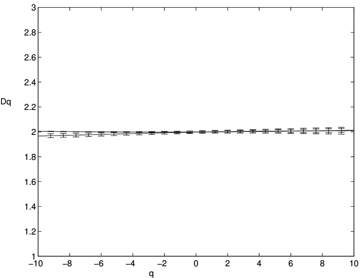
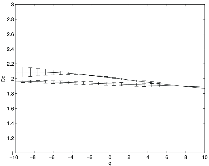
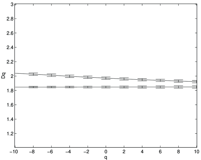
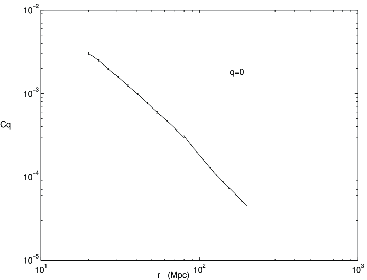
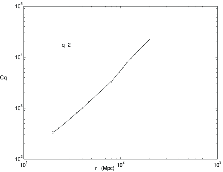
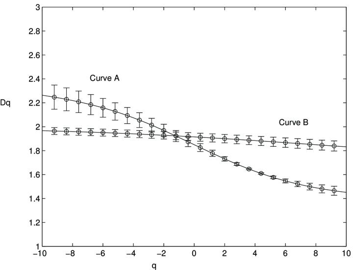
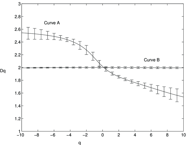
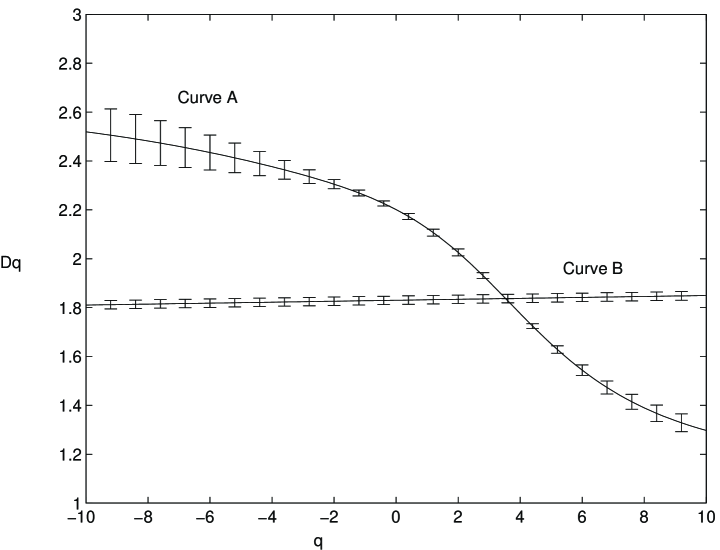
Table 1.

			Absolute	Luminosity	Number of	Vol./Mag.
subsample	$\,\,\,\delta$	z range	Magnitude range	Function	Galaxies	Limited
d-12.1	$-$12.0	0.017-0.2	$-$23.0 - $-$17.5	NS112	4458	M
d-12.2	$-$12.0	0.017-0.2	$-$23.0 - $-$17.5	N112	4458	M
d-12.3	$-$12.0	0.05-0.1	$-$21.0 - $-$20.0	N112	869	V
d-12.4	$-$12.0	0.065-0.125	$-$21.5 - $-$20.5	N112	923	V
d-06.1	$-$6.0	0.017-0.2	$-$23.0 - $-$17.5	NS112	2316	M
d-03.1	$-$3.0	0.017-0.2	$-$23.0 - $-$17.5	NS112	4055	M