Observations of GRB 990123 by the Compton Gamma-Ray Observatory

Abstract

GRB 990123 was the first burst from which simultaneous optical, X-ray and gamma-ray emission was detected; its afterglow has been followed by an extensive set of radio, optical and X-ray observations. We have studied the gamma-ray burst itself as observed by the CGRO detectors. We find that gamma-ray fluxes are not correlated with the simultaneous optical observations, and the gamma-ray spectra cannot be extrapolated simply to the optical fluxes. The burst is well fit by the standard four-parameter GRB function, with the exception that excess emission compared to this function is observed below $\sim 15$ keV during some time intervals. The burst is characterized by the typical hard-to-soft and hardness-intensity correlation spectral evolution patterns. The energy of the peak of the $\nu f_{\nu}$ spectrum, $E_{\rm p}$, reaches an unusually high value during the first intensity spike, $1470\pm 110$ keV, and then falls to $\sim$300 keV during the tail of the burst. The high-energy spectrum above $\sim 1$ MeV is consistent with a power law with a photon index of about $-3$. By fluence, GRB 990123 is brighter than all but 0.4% of the GRBs observed with BATSE, clearly placing it on the $-3/2$ power-law portion of the intensity distribution. However, the redshift measured for the afterglow is inconsistent with the Euclidean interpretation of the $-3/2$ power-law. Using the redshift value of $\geq 1.61$ and assuming isotropic emission, the gamma-ray fluence exceeds $10^{54}$ ergs.

1. INTRODUCTION

GRB 990123 was the first gamma-ray burst to be simultaneously detected in the optical band. The Robotic Optical Transient Search Experiment (ROTSE) detected optical emission during the burst and also immediately after gamma-ray emission was no longer detectable (Akerlof et al. 1999a,b). Observations of prompt X- and gamma-rays were made by several spacecraft, including all four instruments on the Compton Gamma-Ray Observatory, and the Wide Field Camera on Beppo-SAX (Feroci et al. 1999). The burst’s afterglow was detected and monitored at X-ray (Heise et al. 1999), optical (Odewahn et al. 1999) and radio (Frail et al. 1999) energies, resulting in the rapid localization of the burst (Piro et al. 1999; Heise et al. 1999), the determination of the redshift ($z\geq 1.61$—Kelson et al. 1999; Hjorth et al. 1999), and the characterization of the afterglow’s spectrum and evolution (Galama et al. 1999, Fruchter et al. 1999b, Kulkarni et al. 1999, Sari & Piran 1999b). This extensive set of observations permits an analysis of the burst’s relation to its afterglow. Here we present an analysis of the observations obtained with the instruments on the Compton Gamma-Ray Observatory (CGRO). Our goals are to: a) relate the X-ray and gamma-ray spectra to the optical flux; b) to characterize the burst, comparing it to other bursts, and c) to discuss the implications of this event.

According to the currently favored class of theoretical models, the observed burst and subsequent afterglow radiation are synchrotron emission by non-thermal electrons accelerated by strong shocks in relativistic outflows (Rees & Mészáros 1992; Galama et al. 1998; see Piran 1999 for a review). In this model, the high-energy emission of the burst itself is radiated by “internal shocks” which result from the collisions between regions with different velocities (Lorentz factors) within the relativistic outflow, while the lower energy (radio, optical and X-ray) afterglow is thought to be emitted by an “external shock” where the outflow plows into the surrounding medium. Mészáros & Rees (1997) and Sari & Piran (1999a) pointed out that when the external shock first forms, a reverse shock propagates back into the relativistic outflow; the shocked region behind the reverse shock is denser and somewhat cooler than the region behind the external shock, and radiates in the optical band. The optical emission from the reverse shock will be visible during or soon after the high-energy burst produced by the internal shocks.

Multi-wavelength observations during and immediately after the burst can test the current theoretical model’s predictions by detecting the transitions between the emissions from the different regions. Soft X-ray tails, possibly the beginning of the X-ray afterglow, are sometimes observed after higher energy emission has ended (e.g., Yoshida et al. 1989; Sazonov et al. 1998). The X-ray emission at the end of GRB 970228 (Costa et al. 1997) and GRB 980329 (in’t Zand et al. 1998) is consistent with an extrapolation of the X-ray afterglow decay observed many hours after the burst, suggesting that the burst merges smoothly into the afterglow. GRANAT/SIGMA observed a $t^{-0.7\pm 0.03}$ power law decay of the 35–300 keV light curve for 1000 s following GRB 920723 (after which the extrapolated flux would have been undetectable—Burenin et al. 1999); the power law begins immediately after the burst appears to end, when there is an abrupt change in the gamma-ray spectral index from 0 to $-1$ (i.e., to $N_{E}\propto E^{-1}$). In prompt pointed observations OSSE detected significant persistent emission above 50 keV ($\geq 300$ keV in some cases) following the main burst in four of five events in a fluence selected sample (Matz et al. 1999). The emission was detectable for $10^{2}$–$10^{3}$ s with decays consistent with the power-law declines seen in the afterglows at lower energies. There was no evidence for a significant gap between the end of the burst and the beginning of the persistent emission. BATSE observations of GRB 980923 show a power-law decay in time of the emission above 25 keV between about 40 and 400 s after the beginning of the burst—this decay appears to be a higher-energy analog of the x-ray afterglows seen in other events (Giblin et al. 1999). On the other hand, the X-ray light curve of GRB 780506 observed by HEAO-1 shows a period of a few minutes without detected flux after the burst, followed by renewed emission, suggesting a gap between X-ray emission from the burst and from the afterglow (Connors & Hueter 1998).

The ROTSE detection of optical flux simultaneous with the gamma-ray emission and during the $\sim 10$ minutes following the burst (Akerlof et al. 1999a,b) can probe the issue of which physical regions radiate when. These optical observations consisted of three 5 s exposures beginning 22.2, 47.4 and 72.7 s after the trigger of CGRO’s Burst and Transient Source Experiment (BATSE) at 35216.121 s UT on 1999 January 23 (see Fig. 1), and three 75 s exposures beginning 281.4, 446.7 and 612.0 s after the trigger. Gamma-ray emission was detected for about 100 s, so the last three optical detections by ROTSE occurred after the apparent end of the burst phase of the GRB. ROTSE uses an unfiltered CCD, but an equivalent V band magnitude is reported; we will use these magnitudes without attempting any color corrections, etc. The optical flux increased from the first to the second exposure ($m_{v}=11.82$ to $m_{v}=8.95$), and then decayed from exposure to exposure ($m_{v}=10.08$, 13.22, 14.00 and 14.53).

All four CGRO instruments detected this burst (however, the spark chamber of EGRET was not operating); in fact, ROTSE responded to a preliminary BATSE position. Here we describe the spectral evolution of the burst, and compare its spectrum with the optical flux measurements. In §2 we describe our analysis of the CGRO observations of GRB 990123, while in §3 we discuss the implications of this analysis for burst models.

2. DATA ANALYSIS

2.1. Multi-instrument analysis

The CGRO instruments observed GRB 990123 at different energies and time scales. Here we present our procedures and some general results; more detailed discussion of the data of each instrument appears in the following subsections.

Figure 1 shows the light curve in different energy bands accumulated by BATSE and COMPTEL, the two instruments with the best combination of temporal and spectral resolution for this purpose. The light curves show that the low-energy emission persists longer than high-energy emission—typical “hard-to-soft” spectral evolution. Particularly striking is the virtual absence of high-energy emission 45–90 s after the burst trigger. In the highest energy band shown, 4 to 8 MeV, emission is seen from the first spike but appears to be absent or much reduced in the second, providing evidence that the first spike is harder than the second. The first spike also appears narrower in the 4 to 8 MeV band, even compared to the 2 to 4 MeV band.

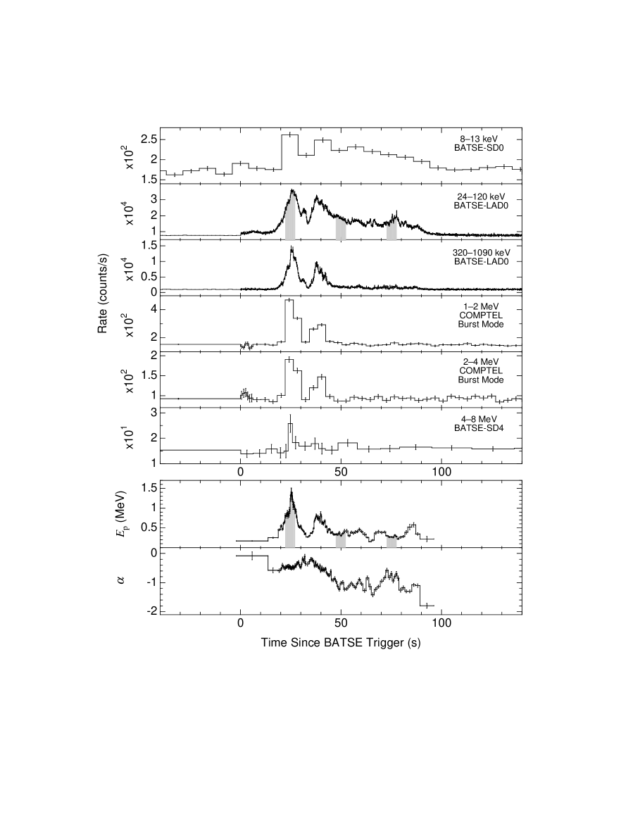
Figure 1.— Top six graphs: Time history of GRB 990123 using data from CGRO detectors. The intervals over which the first three ROTSE observations were accumulated are indicated with shaded bands. Lower two graphs: The time evolution of $E_{\rm p}$, the energy of the peak of $\nu f_{\nu}$, and of $\alpha$, the low-energy photon index in the GRB function. These parameters were obtained from GRB function fits to MER 16 channel spectra from BATSE LADs 0 and 4. The horizontal bars on the points show the time over which the spectrum was fit, and the vertical bars show the $1\sigma$ uncertainty in the values.

Fitting models to spectra provides the most accurate characterization of spectral evolution, although fits are possible only for spectra with a sufficiently large signal-to-noise ratio (S/N). For fitting the BATSE data we use the “GRB” function (Band et al. 1993), which consists of a low-energy power law with an exponential cutoff, $N_{E}\propto E^{\alpha}\exp[-E(2+\alpha)/E_{\rm p}]$, which merges smoothly with a high-energy power law, $N_{E}\propto E^{\beta}$. The “hardness” of this spectrum can be characterized by the energy $E_{\rm p}$ of the peak of $E^{2}N_{E}\propto\nu f_{\nu}$ for the low-energy component (if $\beta<-2$, as is the case for GRB 990123, then $E_{\rm p}$ is the peak energy for the entire spectrum). Most of the spectral curvature is found in the observations made with BATSE below about 1 MeV; the spectra above $\sim$ 1 MeV from the other instruments are consistent with a simple power-law, which we identify as the high-energy power law $E^{\beta}$ of the GRB function.

The model fitting is done using the standard forward-folding technique (see review by Briggs 1996). Briefly, for each instrument we assume a photon model (‘GRB’ for BATSE, power law for the other instruments) and convolve that photon spectrum through a detector model to obtain a model count spectrum. The model count spectrum is compared to the observed count spectrum with a goodness-of-fit statistic, and the photon model parameters are optimized so as to minimize the statistic. In most cases $\chi^{2}$ is used as the goodness-of-fit statistic. This procedure is model dependent. Presenting a comparison of the data and model in count space is the best way to show the quality of the fit. However, it is difficult to show results from all four instruments on one count-rate figure because of the widely differing responses of the instruments. We therefore present photon spectra: the photon “datapoints” are calculated by scaling the observed count rate in a given channel by the ratio of the photon to count model rate for that channel; this ratio and therefore the photon datapoints are model dependent.

An additional complication is that the differing time boundaries of the spectral data from the CGRO instruments preclude forming a multi-instrument spectrum for exactly the same time interval. We have therefore selected time intervals which are as similar as possible and which include the two spikes of the burst (see Table 1). At high energies the flux of the spikes is much higher than the flux of non-spike intervals, consequently as long as each spectrum includes the spikes, differences in the time boundaries are relatively inconsequential, excepting that the spectra must be normalized to a common time interval encompassing the spikes. Because of the small differences expected from the differing time intervals and because of inter-detector calibration uncertainties, we have not attempted simultaneously fitting the data from different instruments with the same photon model.

Table 1Multi-Instrument Spectral Analysis

		Integration Times			Energy Range			Model Normalization
instrument	detector	start	end	length	low	high	$\beta$	at 1 MeV
		(s)	(s)	(s)	(MeV)	(MeV)		($\gamma$ cm-2 s-1 MeV-1)
BATSE	LAD 0	12.288	45.056	32.768	0.033	1.80	$-3.11\pm 0.07$	$1.93\pm 0.02$
BATSE	SD 0 disc.	12.288	45.056	32.768	0.008	0.013
BATSE	SD 1 disc.	12.288	45.056	32.768	0.015	0.030
BATSE	SD 4	12.736	44.928	32.192	0.320	25.
OSSE	Detector 2	12.288	45.056	32.768	1.0	10.	$-2.82\pm 0.16$	$1.68\pm 0.23$
COMPTEL	BSA	14.199	46.398	32.199	1.0	8.5	$-2.78\pm 0.16$	$1.49\pm 0.10$
COMPTEL	telescope	13.331	46.099	32.768	0.75	30.	$-3.33\pm 0.26$	$2.0\pm 0.26$
EGRET	TASC	$-$0.057	64.503	64.560	0.97	250.	$-2.71\pm 0.08$	$1.09\pm 0.07$

The resulting photon spectra are shown in Figure 2. The overlap between instruments is at the upper-end of the break region and in the high-energy power law regime. The overall agreement between the four instruments and the six detector types is very good. Data from the BATSE detectors, LAD 0 and SD 4, overlap from 0.32 to 1.8 MeV and are in excellent agreement except for the highest energy LAD point at 1.1 to 1.8 MeV. The most discordant points are the highest energy point from BATSE LAD 0 and the two lowest energy points from the EGRET TASC. Because of the very small statistical uncertainties on these three points, systematics in the calibrations probably dominate. The values of the high-energy spectral index $\beta$ obtained by the instruments are largely consistent (Table 1). There are larger differences between the model normalizations (Table 1). Differences in the normalizations at the level of $\sim 10\%$ are expected because of uncertainties in the effective areas. The assumption of a simple power-law for the OSSE, COMPTEL and EGRET fits, despite the presence of some curvature in the lowest energy data of these instruments, also contributes to the discrepancies.

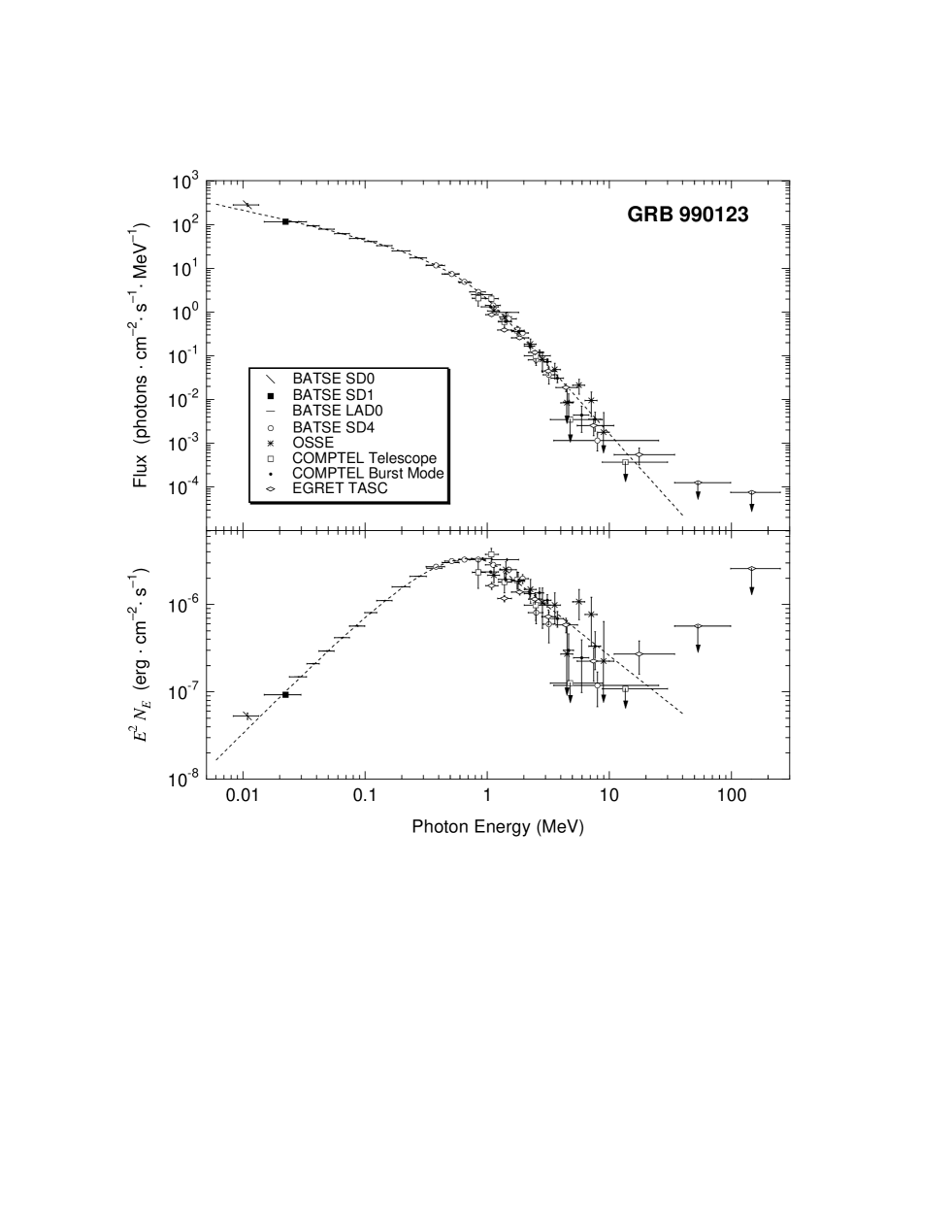
Figure 2.— Deconvolved spectra from the CGRO detectors, shown both as photon flux $N_{E}$ and in $E^{2}N_{E}=\nu f_{\nu}$ units. The spectra have been rebinned into wider bins for clarity. Each spectra is calculated using the actual accumulation times (Table 1), except for the EGRET TASC spectrum, which uses a shorter time interval during which the emission was intense (see text)

2.2. BATSE

The different BATSE datatypes provide varying temporal and spectral resolution. Each of the eight BATSE modules contains a Large Area Detector (LAD), a relatively thin 2000 cm² NaI crystal, and a Spectroscopy Detector, a 12.7 cm diameter by 7.6 cm thick NaI crystal. The large area of the LADs permit high temporal resolution analyses, at limited spectral resolution, while the Spectroscopy Detector (SD) permit higher spectral resolution studies. The LADs are all operated with the same detector settings but the SDs are run at different gain settings and therefore cover a variety of energy ranges. Spectra are accumulated more frequently for the modules with higher count rates. Fortunately, the SD with the greatest count rate, SD 0, was in a high gain state, resulting in spectra from $\sim 25$ to 1750 keV (“SHERB” spectra), as well as a calibrated discriminator channel (“DISCSP1”) between 8 and 13 keV. SD 0 was at a burst angle of 35.2^∘. The second “rank” detector, SD 4, was at a burst angle of 53.8^∘; with a low gain setting, SD 4 provided spectra between 320 keV and 25 MeV. A discriminator channel between 15 and 27 keV was obtained from the third rank detector SD 1 at an angle of 58.6^∘.

The LADs provide data from about 33 to 1800 keV in 16 channels. For Fig. 2, we use the CONT data from LAD 0, which provides 2.048 s resolution. The MER datatype from the LADs provide rates in the same 16 channels every 16 ms for the first 32.768 s of the burst, followed by 64 ms resolution for an additional 131 s. For GRB 990123, the MER data is summed from LADs 0 and 4, which had angles to the burst of $27.5^{\circ}$ and $46.0^{\circ}$, respectively. (For GRB 990123, high time resolution data from the energy channel from 230 to 320 keV is missing due to a telemetry gap; however, all channels are available at 2.048 s resolution via the CONT datatype). These MER rates show the burst’s temporal morphology (see Figure 1), and are particularly useful for studying spectral evolution.

Figure 1 (lower panels) shows the evolution of $E_{\rm p}$ using fits to 16 channel MER spectra from LADs 0 and 4 rebinned in time to provide S/N of at least 100. In order to improve the reliability of the fits, and because there is little evidence for temporal variations in $\beta$, the GRB function was used with $\beta$ fixed at $-3.11$. This value of $\beta$ was obtained from the joint fit to the BATSE data shown in Fig. 2 and is consistent with the values obtained from the other instruments (see Table 1). As can be seen, $E_{\rm p}$ increases by a large factor every time there is a spike in the light curve, as is typical of “hardness-intensity” spectral evolution. Additionally, the maximum $E_{\rm p}$ is greater in the first spike than in the second, $E_{\rm p}$ decreases more rapidly than the count rate and has an overall decreasing trend, behaviors which are typical of “hard-to-soft” evolution (Ford et al. 1995). The small $E_{\rm p}$ maximum for the second spike is consistent with the absence of that spike in the 4 to 8 MeV lightcurve (Fig. 1). Two intervals during the first spike have $E_{\rm p}$ values of $1470\pm 110$ keV. Such values are exceptional—only 3 bursts of the 156 studied by Preece et al. (1999) have spectra with $E_{\rm p}$ values above 1000 keV.

To investigate the burst spectrum over the broadest energy range possible, we extend the LAD spectra by also fitting the SD data. The high-energy resolution SHERB data can be fit satisfactorily by the GRB function discussed above; the fits are consistent with the fits to other data types. SD 4 provides detections of burst flux to at least the 4.0 to 8.0 MeV band (Fig. 1). For the multi-instrument fit shown in Fig. 2, the BATSE data from LAD 0, SD 4 and SD discriminators 0 and 1 are jointly fit to a common photon model, allowing a small “float” in normalization between the detectors (for the discriminators, the relative normalizations are found using the high-resolution data from the same detectors). The relative normalization between LAD 0 and SD 4 is consistent with unity: $1.01\pm 0.01$. The relative normalization differences between the SDs are 10%, which is a typical value. The result of the fit to this 32 s interval is $E_{\rm p}=720\pm 10$ keV, $\alpha=-0.60\pm 0.01$ and $\beta=-3.11\pm 0.07$. At 1 MeV, the fitted flux is $1.93\pm 0.02$ photons cm^-2 s^-1 MeV^-1.

To test for the presence of an X-ray excess in GRB 990123 (as is seen in some other bursts—Preece et al. 1996), we fit the SHERB spectrum and the discriminator channel accumulated by SD 0 over various segments of the light curve, including each of the first three ROTSE observations. We used the GRB function and fit all data points. For SD 0 the discriminator channel covers 8–13 keV, and the SHERB data 26–1760 keV. A significant soft excess above the fit of the GRB function is present in both of the major emission spikes (i.e., between 17.280 and 44.928 s after the BATSE trigger), including the first ROTSE observation, but is not evident in tail of the burst (i.e., after 44.928 s after the trigger), including the second and third ROTSE observations. This soft excess is also not present during the weak emission before the first major emission spike (i.e., up to 14.464 s after the trigger), and surprisingly, during a weak secondary peak on the declining edge of the first emission spike (29.696–34.304 s after the trigger). To verify the presence of the soft excess in the first ROTSE observation, we added the spectrum accumulated by SD 1 which was at a lower gain and therefore covered a higher energy range. In particular, the SD 1 discriminator channel partially covers the gap between SD 0’s discriminator channel and SHERB spectra. As shown by Figure 3, the joint fit is satisfactory, and the X-ray excess is weakly evident in the SD 1 discriminator channel.

     Figure 3.— Fit to SD count spectra for the time interval of the first ROTSE observation. The data points are from the SHERB data of SD 0 and SD 4, and from the low-energy discriminators of SD 0 and SD 1, as indicated. The model photon spectrum, the GRB function, has been folded through the detector response, resulting in the model count spectra (histograms). Each detector, including each discriminator, has a separate count model and therefore a separate histogram. The histogram for each discriminator appears as a horizontal line. Note that the lowest energy discriminator point clearly lies above the GRB model (horizontal line). The spectral parameters of the model are $E_{\rm p}=1170\pm 30$ keV, $\alpha=-0.63\pm 0.02$ and $\beta=-4.1\pm 0.4$.

Integrating spectral fits over the energy range 20–2000 keV provides a measure of the intensity of the high-energy emission. During the three ROTSE observations the photon fluxes are 30.98, 8.17 and 7.74 photons s^-1 cm^-2 while the energy fluxes are $2.14\times 10^{-5}$, $1.68\times 10^{-6}$ and $1.82\times 10^{-6}$ erg s^-1 cm^-2; the ratios of these fluxes show that the average photon energy decreased from the first to the second and third observations. Integrating the GRB function fit to the SHERB spectrum accumulated over the entire burst gives a $>20$ keV fluence of $3.0\times 10^{-4}$ erg cm^-2. The GRBM of Beppo-SAX reported a 40–700 keV fluence of $3.5(\pm 0.4)\times 10^{-4}$ erg cm^-2 (Feroci et al. 1999). The $>20$ keV fluence $5.09(\pm 0.02)\times 10^{-4}$ erg cm^-2 reported by Kippen et al. (1999) was obtained using BATSE 4-channel discriminator data. This technique is less accurate, particularly for hard bursts like GRB 990123, because assumptions about the spectrum must be made in the deconvolution process. These diverse fluence values gives a sense of the consequences of differences in the inter-detector calibrations and analysis methods.

The low-energy SD discriminator channel (DISCSP datatype) extends our spectrum down to 8 keV for SD 0. The WFC on Beppo-SAX covers the energy range 1.5–26 keV. Feroci et al. (1999) report that the WFC flux peaked $\sim 40$ s after the high-energy peak, which would place the WFC peak between the second and third ROTSE observations. The WFC peak intensity of 3.4 Crab corresponds to $\sim 17$ photons s^-1 cm^-2 in their energy band. We fit the DISCSP and SHERB data for SD 0 over $\sim 9$ s around the time of the WFC peak; only the low-energy part of the GRB function was necessary to fit the spectrum. The DISCSP data point was $\sim$40% higher ($\sim 1.5\sigma$) than the model fit, suggesting that there is at most a moderate soft excess. Integrating the model fit over the WFC energy range gives a flux of $\sim 16$ photons s^-1 cm^-2, which is in acceptable agreement with the WFC flux, given the uncertain inter-detector calibration.

2.3. OSSE

The Oriented Scintillation Spectrometer Experiment (OSSE) consists of 4 collimated ($3.8^{\circ}\times 11.4^{\circ}$) NaI detectors covering the  50 keV to  250 MeV energy range. The burst occurred $\sim 20^{\circ}$ and $\sim 60^{\circ}$ outside of the detector’s narrow and broad aperture dimensions, respectively. However, because the burst was intense and hard, radiation penetrated the shielding, permitting a $>1.0$ MeV spectrum to be accumulated. In addition, a high time resolution (16 ms) light curve was recorded above $\sim$0.13 MeV by the NaI shields for the first 60 s of the burst. The time structure is complex with variations observed as short as $\sim$ 16 ms. Light curves can be formed in different energy bands using the photons which penetrated the shields into the detectors. These light curves show that most of the emission above a few hundred keV occurred during the two intensity spikes at the beginning of the burst; this is consistent light curves of BATSE and COMPTEL (Fig. 1). The spectrum appears to extend to the 3–10 MeV band.

The spectrum of these photons can be analyzed, even though they did not originate in the detectors’ field-of-view and were attenuated by the shields, because an appropriate response model was created and tested on solar flares at comparable off-axis angles. The spectrum from Detector 2 suffered the least scattering and attenuation by material in the spacecraft. The background spectrum uses data from 115 s before and after the burst. A power law model was fit to the data, resulting in a 1 MeV flux of 1.68$\pm 0.23$ photons cm^-2 s^-1 MeV^-1 and a photon index $\beta$ of $-2.82\pm 0.16$; this fit was used to create the photon spectrum shown on Figure 2. Integrating this spectrum over the 32.768 s of most of the high-energy emission results in a fluence of $(0.91\pm 0.27)\times 10^{-4}$ erg cm^-2 from 1 to 10 MeV.

2.4. COMPTEL

COMPTEL detected with high significance the two main spikes of GRB 990123 in both its imaging telescope (“double scatter”; 0.75–30 MeV) and non-imaging burst-spectroscopy (“single scatter”; 0.3–1.5 MeV and 0.6–10 MeV) modes. The burst-spectroscopy or BSA mode relies upon two NaI detectors in the bottom layer of the telescope (see Schönfelder et al. 1993 for instrument details).

In imaging telescope mode, COMPTEL provides detailed information on individual time-tagged photons with ${{1}\over{8}}$ ms time resolution. However, for GRB 990123 these telescope data suffered from two limitations: 1) the telescope-mode effective area was at best a few cm² as GRB 990123 occurred nearly 60^∘ from COMPTEL’s pointing direction; and 2) because of the event’s high intensity, even at this low effective area a total of about 16% of this burst’s livetime was lost due to telemetry limits (a maximum throughput of about 20 events per second).

In contrast, the effective area in burst spectroscopy mode was roughly two orders of magnitude greater than in telescope mode, and the deadtime was negligible. However, the spectral accumulation time was set at 4 seconds. Therefore the COMPTEL light-curves displayed in Fig. 1 are from the burst spectroscopy mode. The signal was negligible above 4 MeV. For both telescope and burst spectroscopy modes, the background appeared stable so results depended little (a few %) on the choice of background integration time.

Spectra from the two modes were handled differently. For the 0.75–30 MeV telescope data, one selects only events falling within a certain angle of the source position (“angular resolution measure”, or A.R.M.; Schönfelder et al. 1993), both reducing background and creating a nearly diagonal response (e.g. Kippen et al. 1998). For the telescope spectrum displayed in Fig. 2, a 20^∘ A.R.M. limit was used. The 32.768 s integration interval (see Table 1) was chosen both to cover all the significant gamma-ray emission and to allow the best live-time calculations. The background was taken from 131 seconds of data 15 orbits prior to the burst (see Kippen et al. 1998). These data were fit via the forward-folding technique assuming a simple power-law. Because of the few counts per bin and the background level, the goodness-of-fit statistic used was the background-marginalized Poisson statistic of Loredo (1992). The statistic indicates that this fit is good; however, the data are also consistent with a break at or below 1 MeV (as indicated by the fit to the BATSE data) and also with a break at or above 6 MeV. The best-fit was $2.0\pm 0.26(E/1{\rm MeV})^{-3.33\pm 0.26}$ photons cm^-2 s^-1 MeV^-1, giving a total fluence of $(1.0\pm 0.3)\times 10^{-4}$ ergs cm^-2 (0.75–30 MeV). Systematic errors in the effective area and from deadtime are comparable in magnitude to the statistical errors specified here.

The single detector count spectra obtained in “spectroscopy mode” were processed as follows: the background was estimated from a spectrum of 140 seconds duration starting 202 seconds prior to the BATSE trigger. Eight high range (0.6–10.0 MeV) detector spectra (4 s integration time each) covering a 32 s time interval (Table 1), were background subtracted and summed. For these data, the forward-folding fitting was done using $\chi^{2}$ as the goodness-of-fit criterion. The location of the burst (zenith distance = $56.4^{\circ}$) results in an effective detector area of 541 cm², corresponding to 87% of the on-axis area. Assuming a single power law, the fit to the data from 1.0 to 8.5 MeV (Fig. 2) gives best fit parameter values of normalization = ($1.49\pm 0.10$) photons cm^-2 s^-1 MeV^-1 at 1 MeV and index $\beta$ = $-2.78\pm 0.16$. The fluence (1.0–8.5 MeV, 32 s) is $7.93\times 10^{-5}$ erg cm^-2 We note a clear break of the data below 1 MeV where the spectrum becomes flatter. Preliminary analysis of the low range (0.3–1.5 MeV) spectroscopy data (not shown in Fig. 2) covering the same 32 s time interval also indicates a spectral break at around 0.8 to 1 MeV.

2.5. EGRET

The Energetic Gamma-Ray Experiment Telescope (EGRET) has two methods of detecting gamma-ray bursts. The EGRET spark chambers are the primary detector for the telescope and are sensitive to gamma rays above 30 MeV. The spark chamber detector is turned on in response to an onboard trigger provided by BATSE when a burst is detected within 40 degrees of EGRET’s principal axis. However, GRB 990123 was too far off axis (56.4^∘), so no information is available from the spark chambers for this burst.

EGRET also detects gamma-ray bursts with the Total Absorption Shower Counter (TASC), a $77\times 77\times 20$ cm NaI(Tl) detector. While acting principally as the calorimeter for the spark chambers, it is also an independently triggered detector in the energy range from 1 to 200 MeV. The TASC is unshielded from charged particles and has a high background rate, which is determined from the time intervals just preceding and following the burst. The response of the TASC varies strongly with incident angle, because of the intervening spacecraft material. An EGS-4 Monte Carlo code is used with the CGRO mass model to determine the response of the detector as a function of energy and incident photon direction. In normal mode a spectrum is accumulated every 32.768 seconds. Shorter time intervals are also accumulated following a BATSE burst trigger; however, these short intervals were prior to the peak of this burst since BATSE triggered $\approx$ 25 seconds prior to the peak of the emission.

The burst was detected in the EGRET TASC in two successive 32.768 second intervals. The first is from $-$0.057 to 32.711 s relative to the BATSE trigger, the second from 32.735 to 65.503 s. The break between the two records occurs roughly between the two major spikes. The differential photon spectrum is well fit by a power law, $F(E)=k(E/1{\rm MeV})^{\beta}$, in each separate time interval as well as when the intervals are combined. The combined 65.5 second interval (Fig. 2) is fit by $\beta=-2.71\pm 0.08$ and $k=1.09\pm 0.07$ photons cm^-2 s^-1 MeV^-1. The normalization $k$ and the points in Fig. 2 are calculated assuming that the excess flux above background was emitted over 32.7 s, the time interval of the high energy emission from the burst as seen in the light curves of BATSE and COMPTEL shown in Fig. 1.

The separate spectral fits of the two major spikes show no evidence of spectral evolution. The differential photon spectral index, $\beta$, for the first spectrum is $-2.56\pm 0.11$, and for the second is $-2.78\pm 0.15$. The normalization $k$ is $0.97\pm 0.08$ for the first spectrum and $1.20\pm 0.13$ for the second spectrum, where the time intervals for the emissions of the first and second spectra are assumed to be 20.4 s and 12.3 s, respectively.

3. DISCUSSION

3.1. Optical

The detection of simultaneous optical emission with ROTSE is the primary distinction of GRB 990123, and the obvious question is the relationship between the optical and gamma-ray fluxes. The optical and gamma-ray light curves are clearly very different: the optical flux rose by an order of magnitude from the first to second observation, and then fell by a factor of 2.5 to the third one. On the other hand, the first optical observation occurred during the first hard gamma-ray spike, while the second and third observations occurred during the soft tail after the two main gamma-ray spikes. Indeed, the 20–2000 keV energy flux, calculated by integrating over fits to the spectrum, is an order of magnitude higher during the first optical observation than during the subsequent two, which had comparable fluxes. Thus the optical and high-energy fluxes are not directly proportional.

But perhaps the optical and gamma-ray emission are part of one component, and the relative fluxes change as the spectrum evolves? Figure 4 shows the observed optical and gamma-ray spectra for the three observations. The curves show the photon models obtained from fitting the BATSE data. Note the extent of the X-ray excess on Figures 2, 3 and 4. As can be seen, the gamma-ray spectra do not extrapolate down to the optical band without an unseen break or bend. We have included the maximum $3\sigma$ variations in the low-energy gamma-ray spectrum permitted by the data; these extrapolations underestimate the optical flux by an order of magnitude or more. Perhaps the optical emission and the X-ray excess observed during the first ROTSE observation are part of the same component? We extrapolated a power law with index $\alpha_{ox}=-0.243$ connecting the optical and 10 keV X-ray fluxes during this first observation. Figure 4 shows that a similar power law over predicts the X-ray flux by more than an order of magnitude during the second and third optical observations. We conclude that the optical emission is in excess of the low-energy extrapolation of the burst spectrum, which suggests that the optical and high-energy emission originate from different shocks in the relativistic outflow.

     Figure 4.— Optical flux and gamma-ray spectra for the time intervals of the 3 ROTSE observations. The curves for the first (third) time interval have been shifted up (down) by a factor of 1000. The data points “*” on the left are the ROTSE observations, while the solid curves on the right are the best fit models to the BATSE SD spectra. The dashed curves on the low-energy end of the gamma-ray spectra show the spectra for $3\sigma$ variations in $\alpha$, the GRB function’s low-energy spectral index. The dot-dashed curve is the extrapolation of the optical flux to 10 keV using $\alpha_{ox}$, the power law index connecting the observed optical and 10 keV X-ray fluxes for the first ROTSE time interval.

3.2. X-Ray Emission

Also interesting is the observation that the X-ray excess and the gamma-ray emission are apparently not related. That is, the excess occurs during the two main spikes in the gamma-ray time history, but not in the time interval afterwards, as well as being absent during a small flaring episode on the falling portion of the first main spike. The X-ray time history in the 8–13 keV band shows interesting behavior during the tail end of the burst: rather than the flat shoulder present in the gamma-rays, there is a somewhat steady fall-off in flux from T$+50$ s to T$+130$ s. At the same time, the low-energy power-law index $\alpha$ makes a transition from $\sim-0.5$ to $\sim-1.0$ (see Fig. 1). Thus, the portion of the burst associated with the X-ray excess is also associated with a hard low-energy power-law index; when the low-energy index softens, the excess disappears. A possible reason is that the change in slope $\alpha$ causes the X-ray extension of the gamma-ray spectrum to mask the low-energy excess. However, the flux predicted by the GRB function fit to the data of the second ROTSE interval is inadequate to mask the X-ray excess observed during the first ROTSE interval. This suggests that the X-ray component has disappeared by the second half of the burst—making GRB 990123 the first burst in which BATSE has reported evolution in this component. In that case, it is interesting that the X-ray excess is not correlated with the optical emission, which peaks during the second half of the burst.

There are several burst models that support the existence of excess X-rays simultaneously with prompt burst emission. The most successful of these, the Compton attenuation model (CAM—Brainerd 1994), predates the discovery of the excess. In this model, a beam of photons is scattered out of the line of sight by an optically-thick medium via Compton scattering in the Klein-Nishina limit, which is less efficient at higher photon energies than Thompson scattering. It is this change in efficiency that modifies an assumed input power-law spectrum into the observed shape, with a universal break energy in the rest frame determined by the physics. The low-energy upturn is determined by the density of the intervening scattering material. In the simplest form of the CAM, there is no allowance for changes in the optical depth as a function of time, yet the change in amplitude of the X-ray upturn in the present burst seems to require this. When we fit the BATSE spectral data for the first ROTSE interval with the CAM, a $\chi^{2}$ value of 511 for 400 degrees of freedom is obtained. Values of reduced $\chi^{2}$ above unity are typical of very bright bursts like GRB 990123 because systematic deviations dominate the statistical fluctuations. The best-fit value for the red-shift is 1.19 $\pm 0.06$; while $\chi^{2}$ increases by 27 to 538 when the red-shift is required to be 1.61. When the GRB model is fit to all of the BATSE data, including the SD discriminator points with their evidence for an X-ray excess, the same $\chi^{2}$ value of 538 is obtained. If the SD discriminator data are ignored, the GRB model has a substantially better $\chi^{2}$ value than the CAM model, indicating the power of these data for testing models with different X-ray predictions.

Other burst models have various levels of compatibility with an excess of X-rays, but few require it. Usually, a separate, lower-energy spectral component would indicate that Compton up-scattering is producing the observed gamma-rays from a seed population of X-rays. One would expect the two components to be highly correlated in time, which is not observed here. The input spectral shape is modified by the distribution of energetic particles that are doing the up-scattering, so one can infer a power-law index for the particles from the photon continuum spectral index. Finally, it is also not clear if there is any connection between the X-ray flux and the burst afterglow, presumably created in this case by a shock formed when relativistically-expanding material from the burst meets material external to the system, such as interstellar material, or the remnant of a wind from the burst’s progenitor (Sari & Piran 1999a). Although the component of the aftershock related to the optical flash (the reverse shock) is not expected to produce any detectable X-ray component, the forward shock is. The observation that the hard X-rays (top lightcurve of Fig. 1), have a maximum after the occurrence of the two main spikes in the gamma-rays, may indicate the peak of the forward shock in this band.

3.3. Afterglow

Park et al. (1997a) introduced three dimensionless statistics to compare optical detections or upper limits with the observed gamma-ray emission. Behind these statistics are implicit assumptions about the relationship between the emission in these two bands. The first two statistics can be calculated only if the high-energy emission is still detectable at the time of the optical emission. Comparing the optical and gamma-ray flux densities $f_{\nu}$ (in units of erg s^-1 cm^-2 Hz^-1), is $R_{1}=f_{\nu}(\nu_{\rm opt})/f_{\nu}(\nu_{\gamma})$, where $\nu_{\rm opt}$ and $\nu_{\gamma}$ are fiducial optical and gamma-ray frequencies (here the V band’s $5.6\times 10^{14}$ Hz and 100 KeV $=2.4\times 10^{19}$ Hz). Comparing the optical flux to the gamma-ray flux density $f_{\gamma}$ (erg s^-1 cm^-2) is $R_{2}=f_{\nu}(\nu_{\rm opt})\nu_{\rm opt}/f_{\gamma}$. Finally, $R_{3}=f_{\nu}(\nu_{\rm opt})/\phi_{\gamma}$ compares the optical flux density to the gamma-ray energy fluence $\phi_{\gamma}$ (erg cm^-2) from the beginning of the burst until the time of the optical observation. $R_{3}$ is relevant and calculable whether or not the high-energy emission is detectable at the time of the optical observations; however the time between the high-energy emission and the optical observation is physically interesting. While these statistics do depend on the fiducial optical and gamma-ray frequencies which are chosen because of detector capabilities, they do not depend on instrumental quantities such as the length of the optical exposure. Table 2 shows the values of these 3 statistics for the 6 ROTSE detections of GRB 990123. Also shown are typical upper limits obtained with the Gamma-Ray Optical Counterpart Search Experiment (GROCSE), ROTSE’s less-sensitive predecessor, and the upper limits for GRB 970223 (Park et al. 1997b) obtained with the Livermore Optical Transient Imaging System (LOTIS), an instrument very similar in design and operation to ROTSE (LOTIS did not attempt to observe GRB 990123 because of bad weather—H.-S. Park, personal communication 1999). As can be seen, the ROTSE detections are below the GROCSE upper limits, but are comparable to the upper limits for GRB 970223. Only with more detections and upper limits from ROTSE, LOTIS and similar instruments will we determine whether GRB 990123’s optical emission was typical.

Table 2Optical–Gamma-Ray Emission Comparison

Obs.	$t$	$f_{\nu}(\nu_{\rm opt})$	$f_{E}(E_{\rm 100keV})$	$f_{\gamma}$	$\phi_{\gamma}$	$R_{1}$	$R_{2}$	$R_{3}$
GRB 990123-1	22.2	$6.79\times 10^{-25}$	$1.07\times 10^{-8}$	$2.14\times 10^{-5}$	$7.78\times 10^{-5}$	$1.53\times 10^{1}$	$1.78\times 10^{-5}$	$8.73\times 10^{-21}$
GRB 990123-2	47.4	$9.55\times 10^{-24}$	$3.93\times 10^{-9}$	$1.68\times 10^{-6}$	$3.05\times 10^{-4}$	$5.87\times 10^{2}$	$3.19\times 10^{-3}$	$3.13\times 10^{-20}$
GRB 990123-3	72.7	$3.37\times 10^{-24}$	$4.13\times 10^{-9}$	$1.82\times 10^{-6}$	$3.39\times 10^{-4}$	$1.97\times 10^{2}$	$1.04\times 10^{-3}$	$9.95\times 10^{-21}$
GRB 990123-4	281.4	$1.87\times 10^{-25}$	—	—	$2.65\times 10^{-4}$	—	—	$7.06\times 10^{-22}$
GRB 990123-5	446.7	$9.12\times 10^{-26}$	—	—	$2.65\times 10^{-4}$	—	—	$3.44\times 10^{-22}$
GRB 990123-6	612.0	$5.60\times 10^{-26}$	—	—	$2.65\times 10^{-4}$	—	—	$2.11\times 10^{-22}$
GROCSE	$\sim 25$	—	—	—	—	$<1.5\times 10^{4}$	$<4\times 10^{-2}$	$<3\times 10^{-18}$
GRB 970223	11	$<1.4\times 10^{-24}$	$1.4\times 10^{-9}$	$6.09\times 10^{-7}$	$4.8\times 10^{-5}$	$<2.4\times 10^{2}$	$<1.3\times 10^{-3}$	$<2.9\times 10^{-20}$

The $R_{3}$ statistic can also compare the optical afterglows to the gamma-ray emission; Table 3 shows $R_{3}$ for $R$ band afterglow emission after 1 day for a number of recent bursts. These values of $R_{3}$ are usually smaller than the detections and upper limits during and immediately after the burst because it is possible to observe the optical transient with large telescopes once the position is known accurately. We would like to use $R_{3}$ values calculated at the same time and optical frequency in the rest frame of the burst. Assuming that the afterglow flux has power law spectrum and temporal decay, $f_{\nu}\propto\nu^{\epsilon}t^{\delta}$, then $R_{3,\hbox{burst}}=R_{3,\hbox{observer}}(1+z)^{\delta-\epsilon}$. For most afterglows $\epsilon\sim\delta\sim-1$ (e.g., Galama et al. 1997, 1998, 1999; Bloom et al. 1998), and by afterglow theory $\delta-\epsilon=(\delta+1)/3$ for adiabatic cooling; thus $R_{3,\hbox{burst}}$ has at most a weak dependence on redshift. As can be seen, there is a wide range of values, which confirms that afterglows are not all alike. Indeed, the $R_{3}$ value and the isotropic gamma-ray energy are inversely correlated, which results from a broader energy distribution than the distribution of $R$ band specific luminosities in the bursts’ frame (i.e., the optical flux converted into a luminosity emitted by the afterglow). This suggests that the efficiency with which the total energy is converted into emission varies with wavelength band. For example, in the standard model, the energy release by internal shocks depends on details of the relativistic flow, which can vary from burst to burst, while the kinetic energy of the flow is expended at the external shock; thus the distribution of afterglow energies may be narrower than that of the burst itself.

Table 3Burst Energetics

GRB	$z$	$\phi_{\gamma}$ ($>$ 20 keV)	$E$	$m_{R}$ (1 day)	$f_{\nu}(\nu_{R})$	$R_{3}$	Ref.
970228		$2.0\times 10^{-6}$		21.1$\pm$0.15	1.12$\times 10^{-5}$	5.6$\times 10^{-23}$	1,2
970508	0.835	3.7$\times 10^{-6}$	5.3$\times 10^{51}$	20.85$\pm$0.05	1.32$\times 10^{-5}$	3.8$\times 10^{-23}$	3,4,5
971214	3.418	1.1$\times 10^{-5}$	2.5$\times 10^{53}$	23.0$\pm$0.22	1.94$\times 10^{-6}$	1.8$\times 10^{-24}$	6,7
980326		$2.2\times 10^{-6}$		23.39$\pm$0.12	1.36$\times 10^{-6}$	6.2$\times 10^{-24}$	8
980329	$\sim$5	5.0$\times 10^{-5}$	2.4$\times 10^{54}$	23.9$\pm$0.2	8.48$\times 10^{-7}$	1.7$\times 10^{-25}$	9,10
980519		$1.1\times 10^{-7}$		21.28$\pm$0.13	9.47$\times 10^{-6}$	8.6$\times 10^{-22}$	11,12
980613	1.096	1.7$\times 10^{-6}$	4.2$\times 10^{51}$	23.2$\pm$0.5	1.61$\times 10^{-6}$	9.5$\times 10^{-24}$	13,14
980703	0.966	4.6$\times 10^{-5}$	8.9$\times 10^{52}$	21.18$\pm$0.10	1.04$\times 10^{-5}$	2.3$\times 10^{-24}$	15,16
990123	1.61	3.0$\times 10^{-4}$	1.6$\times 10^{54}$	20.4$\pm$0.3	2.13$\times 10^{-5}$	7.1$\times 10^{-25}$	this paper

3.4. Intensity

GRB 990123’s fluence $\phi_{\gamma}=3.0\times 10^{-4}$ erg cm^-2 places it firmly on the $N(>\phi_{\gamma})\propto\phi_{\gamma}^{-3/2}$ portion of the fluence distribution—only 0.4% of the bursts observed by BATSE have had higher fluences. By photon peak flux, only 2.5% of BATSE bursts have been more intense. Whatever the intensity measure, peak photon flux $P$ or fluence $\phi_{\gamma}$, the high end of BATSE’s cumulative intensity distribution is a power law with an index of $-$3/2. In the simplest cosmological model standard candle bursts occur at a constant rate per comoving volume; bursts in nearby Euclidean space produce the $\phi_{\gamma}^{-3/2}$ portion of the cumulative peak flux distribution while the bend in this distribution results from bursts at sufficiently high redshift ($z>0.3$) that spacetime deviates from Euclidean. Thus we would expect GRB 990123 to occur at low redshift. However the absorption lines in the optical transient’s spectrum show that $z\geq 1.61$ for GRB 990123 (Kelson et al. 1999, Hjorth et al. 1999). GRB 990123 demonstrates that the $\phi_{\gamma}^{-3/2}$ portion of the peak flux distribution does not originate only in nearby Euclidean space. Consequently, the burst rate per comoving volume must vary with redshift, with the burst rate and cosmological geometry “conspiring” to produce the Euclidean-like $\phi_{\gamma}^{-3/2}$ dependence. Indeed it has been suggested that the burst rate is proportional to the star formation rate (e.g., Wijers et al. 1998; Totani 1997), which has decreased precipitously since the epoch corresponding to $z\sim 1.5$.

The redshift implies that GRB 990123’s energy release was at least $1.6\times 10^{54}$ erg ($H_{0}=70$ km s^-1 Mpc^-1, $\Omega=0.3$ and $\Lambda=0$), if the burst radiates isotropically, comparable to the energy release in GRB 980329, if $z\sim 5$ for this burst (Fruchter 1999). Energy releases are given as isotropic equivalents, even though there are indications of beaming (Fruchter et al. 1999b, Kulkarni et al. 1999, but see Mészáros & Rees 1999) because the beaming angles are unknown. See Table 3 for a list of the energies of the bursts with redshifts. Both GRB 971214 ($z=3.418$—Kulkarni et al. 1998) and GRB 980703 ($z=0.966$—Djorgovski et al. 1998a) had energies of $\sim 10^{53}$ erg while GRB 970508 ($z=0.835$—Metzger et al. 1997; Bloom et al. 1998) and GRB 980613 ($z=1.096$—Djorgovski et al. 1999) had energies of $\sim 6\times 10^{51}$ erg. Thus we see that the standard candle assumption behind the simplest cosmological model is violated, and the intrinsic energy distribution is very broad.

Thus two basic premises of the simplest cosmological model are violated. The burst rate and the energy release distribution must now be determined empirically, with the peak flux distribution providing a constraint on these distributions. Note that it may not be possible to separate the burst rate into independent functions of redshift and energy.

4. SUMMARY

The high-energy emission of GRB 990123 was fairly typical of gamma-ray bursts. The spectrum above 25 keV can be fit satisfactorily by the simple four-parameter GRB function. The parameter $E_{\rm p}$, the energy at which $\nu f_{\nu}$ peaks, reached the unusually high value $1470\pm 110$ keV. The typical spectral evolution patterns of hardness-intensity correlation and hard-to-soft evolution are observed. An X-ray excess is present below $\sim 15$ keV during the early part of the burst, particularly during the first ROTSE observation. The burst’s peak flux and energy fluence place the burst in the top 2.5% and 0.4% of all bursts observed by BATSE; these values also are clearly in the portion of the intensity distribution which appears consistent with the $-$3/2 slope power law expected for sources uniformly distributed in Euclidean space. However, GRB 990123’s redshift of $z\geq 1.61$ shows that the burst originated far beyond nearby Euclidean space. This redshift and the fluence imply an energy release of $\geq 1.6\times 10^{54}$ ergs ($H_{0}=70$ km s^-1 Mpc^-1, $\Omega=0.3$ and $\Lambda=0$), if radiated isotropically. GRB 980329, if at $z\sim 5$ (Fruchter 1999), has a similar energy release; the determination of the redshift of GRB 990123 via spectroscopic lines in the afterglow leaves no doubt that isotropic-equivalent energy releases above $10^{54}$ ergs occur.

The gamma-ray and ROTSE optical fluxes are not correlated, and the gamma-ray spectrum does not extrapolate down to the optical observations. Thus there is no indication that the emissions in these two bands are from the same component. Indeed, the standard burst theory attributes the high-energy emissions to “internal shocks” within a relativistic outflow, and the simultaneous optical emission to a reverse shock that forms when the relativistic outflow plows into the surrounding medium.

Various measures that relate the optical and gamma-ray emissions show that the ROTSE detection of optical emission from GRB 990123 is consistent with the upper limits on simultaneous optical emission from previous bursts. Therefore, only future optical observations by ROTSE, LOTIS and similar robotic systems will determine whether GRB 990123 was typical.

References

- (1) Akerlof, C. W., et al. 1999a, GCN #205
- a (2) ———— 1999b, Nature, in press
- a (42) Band, D., et al. 1993, ApJ, 413, 281
- (4) Bloom, J. S., Djorgovski, S. G., Kulkarni, S. R., & Frail, D. A. 1998, ApJ, 507, L25
- (5) Brainerd, J. J. 1994, ApJ, 428, 21
- (6) Briggs, M. S. 1996, in AIP Conf. Proc. 384, ed. C. Kouveliotou, M. Briggs & G. Fishman, 133
- (7) Burenin, R. A., et al. 1999, A&A, submitted [astro-ph/9902006]
- (8) Connors, A., & Hueter, G. J. 1998, ApJ, 501, 307
- fd (2) Costa, E., et al. 1997, Nature, 387, 783
- (10) Diercks, A., Deutsch, E. W., Wyse, R., Gilmore, G., Corson, C., Castander, F. J., & Turner, E. 1997, IAU Circ. 6791
- (11) Djorgovski, S. G., Kulkarni, S. R., Bloom, J. S., Goodrich, R., Frail, D. A., Piro, L., & Palazzi, E. 1998a, ApJ, 508, L17
- (12) ———— 1998b, GCN #79
- (13) ———— 1998c, GCN #117
- (14) ———— 1999, GCN #189
- (15) Feroci, M., et al. 1999, IAU Circ. #7095
- a (233) Ford, L., et al. 1995, ApJ, 439, 307
- (17) Frail, D. A., et al. 1999, GCN #211
- (18) Fruchter, A. 1999, ApJ, in press [astro-ph/9810224]
- (19) Fruchter, A., et al. 1999a, ApJ, in press [astro-ph/9807295]
- xyz (11) Fruchter, A., et al. 1999b, submitted [astro-ph/9902236]
- (21) Galama, T., et al. 1997, Nature, 387, 479
- (22) ———— 1998, ApJ, 497, L13
- (23) ———— 1999, Nature, in press [astro-ph/9903021]
- (24) Giblin, T., et al., 1999, ApJ, submitted
- (25) Groot, P. J., et al. 1998, ApJ, 502, L123
- (26) Heise, J., et al. 1999, IAU Circ. # 7099
- (27) Hjorth, J., et al. 1999, GCN #219
- a (22) in’t Zand, J. J. M., et al. 1998, ApJ, 505, L119
- (29) Kelson, D. D., Illingworth, G. D., Franx, M., Magee, D., van Dokkum, P. G. 1999, IAU Circ. #7096
- xyz (1) Kippen, R. M., Ryan, J. M., Connors, A., Winkler, C., Schönfelder, V., Kuiper, L., McConnell, M., Varendorff, M., Hermsen, W., and Collmar, W. 1998, Adv. Space Res., 22, No. 7, 1097
- (31) Kippen, R. M., et al. 1999, GCN #224
- (32) Kulkarni, S., et al. 1998, Nature, 393, 35
- xvy (12) Kulkarni, S. R., et al. 1999, Nature, in press [astro-ph/9902272]
- xyz (5) Loredo, T. J., 1992, in Statistical Challenges in Modern Astronomy, ed. G. J. Babu & E. D Fiegelson (New York: Springer-Verlag)
- xyz (6) Matz, S., et al. 1999, ApJ, in preparation
- (36) Mészáros, P., & Rees, M. J. 1997, ApJ, 476, 232
- xyz (13) Mészáro, P., & Rees, M. J., 1999, submitted [astro-ph/9902367]
- (38) Metzger, M., et al. 1997, Nature, 387, 878
- (39) Odewahn, S. C., et al. 1999, GCN #201
- (40) Palazzi, E., et al. 1998, A&A, 336, L95
- a (2) Park, H.-S., et al. 1997a, ApJ, 490, 99
- a (3) ———— 1997b, ApJ, 490, L21
- (43) Piran, 1999, Physics Reports, in press [astro-ph/9810256]
- (44) Piro, L., et al. 1999, GCN #199, #202, #203
- adg (2) Preece, R., et al. 1996, 473, 310
- xzy (21) Preece, R., et al. 1999, ApJ, in preparation
- xyz (20) Rees, M. J., & Mészáros, P. 1992, MNRAS, 258, 41
- f (7) Sari, R., & Piran, T. 1999a, ApJ, submitted [astro-ph/9901338]
- xyz (10) Sari, R., & Piran, T. 1999b, submitted [astro-ph/9902009]
- (50) Sazonov, S. Y., Sunyaev, R. A., Terekhov, O. V., Lund, N., Brandt, S., & Castro-Tirado, A. J. 1998, A&ASuppl., 129, 1
- xyz (7) Schönfelder, V. et al., 1993, ApJS, 86, 629
- (52) Totani, T. 1997, ApJ, 486, L71
- (53) Vrba, F. J., et al. 1998, GCN #83
- (54) Vreeswijk, P. M., et al. 1999, ApJ, in press
- (55) Wijers, R. A. M. J., et al. 1998, MNRAS, 294, L13
- (56) Yoshida, A., et al. 1989, PASJ, 41, 509