Constraining the spectral parameters of RX J0925.7–4758 with the BeppoSAX LECS

Abstract

The Super Soft Source RX J0925.7–4758 (RX J0925 hereafter) was observed by BeppoSAX LECS and MECS on January 25–26 1997. The source was clearly detected by the LECS but only marginally detected by the MECS. We apply detailed Non-Local Thermodynamic Equilibrium (Non-LTE) models including metal line opacities to the observed LECS spectrum. We test whether the X–ray spectrum of RX J0925 is consistent with that of a white dwarf and put constraints upon the effective temperature and surface gravity by considering the presence or absence of spectral features such as absorption edges and line blends in the models and the observed spectrum.

We find that models with effective temperatures above $\sim 10^{6}\mbox{ K}$ or below $\sim 7.5\times 10^{5}\mbox{ K}$ can be excluded. If we assume a single model component for RX J0925 we observe a significant discrepancy between the model and the data above the Ne ix edge energy at 1.19 keV. This is consistent with earlier observations with ROSAT and ASCA. The only way to account for the emission above $\sim 1.2\mbox{ keV}$ is by introducing a second spectral (plasma) component. This plasma component may be explained by a shocked wind originating from the compact object or from the irradiated companion star.

If we assume $\log g=9$ then the derived luminosity is consistent with that of a nuclear burning white dwarf at a distance of $\sim 4$ kpc.

1 Introduction

1.1 Supersoft X–ray Sources

Observed with low spectral resolution satellites like Einstein and ROSAT, Supersoft X-ray Sources (SSSs) show heavily absorbed featureless spectra. They are generally characterized by the ROSAT hardness ratio of

$${\rm HR1}\equiv{{\rm H-S}\over{\rm H+S}}\leq-0.8,$$

where H and S are the count rates between 0.5–2.0 keV and 0.1–0.4 keV respectively. This implies that the bulk of the observed photons have energies below 0.5 keV. When fitted with blackbody spectra SSS temperatures typically lie in the range $1.5-5\times 10^{5}\mbox{ K}$. The derived column densities are of the order of $n_{\rm H}=10^{20}-10^{22}\mbox{ cm}^{-2}$. Many of the SSSs have now been optically identified, covering a range of different objects including e.g. classical novae, symbiotic novae and the central star of the planetary nebula N67. Thus SSSs probably do not form a homogeneous class but they may all contain a hot white dwarf which emits the observed soft X–rays. They are commonly believed to be nuclear burning white dwarfs. The nuclear fuel is supplied by a main sequence (or a slightly evolved) companion star or, in the case of N67, by primordial hydrogen and helium left after the asymptotic giant branch phase. This accretion takes place in a very narrow range of rates between $3\times 10^{-8}$ and $7\times 10^{-7}{\rm M}_{\odot}\>\mbox{yr}^{-1}$. For the steady burning SSSs this accretion rate is critical: at lower accretion rates white dwarfs show nova-like behavior. At higher rates white dwarfs develop a strong wind that compensates for the accretion rate (Paczyński & $\dot{\rm Z}$ytkow pazy (1978); Sion et al. sion (1979); Sienkewicz sien (1980); Hachisu et al. hachisu (1996)).

CAL87 and RX J0925.7–4758 (RX J0925 hereafter) are the only two sources which have substantial count rates above 0.5 keV up to $\sim 1.0\mbox{ keV}$. Those sources are fitted with relatively high temperatures of $\la 7.5\times 10^{5}\mbox{ K}$ and $\la 9\times 10^{5}\mbox{ K}$ respectively. Fig. 1 shows the luminosity versus temperature for several SSSs with known temperature and luminosity. Data are taken from Kahabka & Van den Heuvel (kah_heu (1997)). Also indicated are two dashed lines which represent the luminosity at $2.5\times 10^{8}\mbox{ and }5\times 10^{9}\mbox{ cm}$ radius respectively in the relation $L_{\rm bol}=4\pi R^{2}\>\sigma T^{4}$. This range in radius applies to white dwarfs. Note that most SSSs lie within this range. The lower limit for the radius corresponds to the Chandrasekhar upper mass limit for white dwarfs of $1.4M_{\sun}$, applying the mass-radius relation derived by Kahabka & Portegies Zwart (spz (1999)). RX J0925 is shown in the same figure assuming a distance to the source of 1 kpc. Temperature and luminosity bounds have been derived by Hartmann & Heise (hartmann (1997)) by fitting model atmosphere spectra to ROSAT PSPC data of RX J0925. Though a good fit was obtained ($\chi^{2}=0.78$) the derived normalization of the model which is defined as $R^{2}/D^{2}$ is obviously too low, $R$ is the radius of the compact object and $D$ is 1 kpc. A small radius for the compact object (less than $\sim 1000$ km) poses a problem for the white dwarf hypothesis. It has been suggested that RX J0925 is at a distance of 10 kpc in order to account for the factor $\sim 100$ needed to increase the luminosity into the regime bounded by the two dashed lines in Fig. 1 and thus to obtain a model for RX J0925 consistent with a white dwarf (Ebisawa et al. 1996b ; Motch motch3 (1998)).

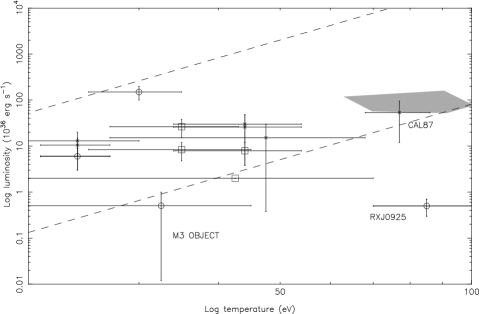
Figure 1: Luminosity versus temperature for several SSSs. Crosses: LMC sources. Squares: SMC sources. Circles: Galactic sources. The dashed lines indicate the relation $L_{\rm bol}=4\pi R^{2}\>\sigma T^{4}$ for $R\approx 2.5\times 10^{8}\mbox{ cm}$ (lower line) for the most massive white dwarfs and $5\times 10^{9}\mbox{ cm}$. A distance of 1 kpc has been assumed for RX J0925. Data are taken from Kahabka & Van den Heuvel (1997). For the explanation of the shaded area we refer to the text in Sect. 4.2

In order to be able to constrain the model parameters more tightly than was previously possible with the ROSAT PSPC and to test whether RX J0925 can be consistent with a white dwarf, RX J0925 was observed with BeppoSAX. We have refined our previous model spectra fitted to RX J0925 by including line opacities in the model atmospheres. In this Paper we describe the data analysis of this observation.

1.2 RX J0925

The Supersoft X–ray Source RX J0925 was discovered in the ROSAT Galactic Plane Survey (RGPS, Motch et al. motch1 (1991)). This survey is defined as the $\mid\!b\!\mid\leq 20\degr$ region of the ROSAT All Sky Survey. By fitting a blackbody to the ROSAT observation a column density of $n_{\rm H}=(1.4-3.7)\times 10^{22}\mbox{ cm}^{-2}$ was derived. Optical observations indicate $n_{\rm H}=(1.0-1.9)\times 10^{22}\mbox{ cm}^{-2}$. This relatively high column density indicates that the source is located within or behind the nearby Vela Sheet molecular cloud (Motch et al. motch2 (1994)). This puts RX J0925 at a distance of at least 425 pc. The galactic coordinates are $\mbox{l\sc ii}=271\aas@@fstack{\circ}36\mbox{ and b\sc ii}=1\aas@@fstack{\circ}88$. Considering this low latitude one can conclude that RX J0925 is a galactic source. A transient jet with a peak jet velocity of $5200\mbox{ km s}^{-1}$ was detected from optical observations. This is compatible with the escape velocity of both a massive white dwarf (Motch motch3 (1998)) and a shrouded neutron star with an extended photosphere of a few thousand kilometers (Greiner greiner91 (1991)).

Ebisawa et al. (1996a ) observed RX J0925 with the ASCA Solid-state Imaging Spectrometer (SIS) in December 1994. A single blackbody spectrum does not fit their data. Applying additional absorption edges at $\sim 0.9$, 1.0 and 1.4 keV and reducing the abundances of interstellar oxygen and iron to A(O) = 0.38 and A(Fe) = 0.2 times solar result in an acceptable fit. The edges at $\sim 0.9$ and 1.4 keV suggest the presence of atmospheric O viii and Ne x or Fe xviii. However, the O viii edge is coincident with the interstellar neon absorption edge and its identification is therefore not unambiguous. The origin of a possible edge at $\sim 1.0\mbox{ keV}$ remains unclear and the observed spectral shape around $\sim 1\mbox{ keV}$ may be due to strong line opacities as well. Preliminary fits of Non-Local Thermodynamic Equilibrium (Non-LTE) model spectra at $\log g=9.0\mbox{ cm s}^{-2}$ to ASCA–SIS data show a strong Ne ix edge in the model which is not observed in the data and a small normalization of 160 km (D/kpc). The fitted effective temperature and column density are $\sim 8.5\times 10^{5}\mbox{ K and }1.0\times 10^{22}\mbox{ cm}^{-2}$ respectively (Ebisawa et al. 1996a ). These parameters are consistent with those derived by Hartmann & Heise (hartmann (1997)) from the ROSAT PSPC observation.

2 BeppoSAX observation of RX J0925

RX J0925 was observed on January 25–26 1997 with the Low and Medium Energy Concentrator Spectrometer (LECS and MECS respectively) aboard BeppoSAX. The LECS energy resolution is a factor $\sim 2.4$ better than that of the ROSAT PSPC, while the effective area is about a factor $\sim 20\mbox{ to }5$ lower at 0.28 and 1.5 keV respectively. Since the LECS can only be operated during satellite night-time, the LECS observed RX J0925 for only 44 ksec. RX J0925 is clearly detected with the LECS as an on-axis source with an average net count rate of $0.074\pm 0.002\mbox{ cts s}^{-1}$.

We rebinned the spectral data to ${1\over 3}\times$ FWHM of the spectral resolution quoted by Parmar et al. (parmar2 (1997)) and Boella et al. (boella (1997)). Moreover, we require a minimum of 20 counts per energy bin to allow the use of the $\chi^{2}$ statistic. The resulting 18 energy bins are used for spectral analysis. The standard on-axis 35 pixel radius region, which is supplied together with the BeppoSAX data analysis package, is used for extracting source photons. Background photons are subtracted applying the same 35 pixel region to a BeppoSAX deep field exposure. During the 103 ksec. exposure with the MECS RX J0925 is only marginally detected on-axis in the 1.3 – 2.0 keV energy band with an average count rate of $0.0022\pm 0.0006\mbox{ cts s}^{-1}$. Above 2.0 keV RX J0925 is not detected with the MECS. In this paper we will therefore focus our attention upon the LECS data.

3 White dwarf model spectra

Table 1: Overview of the model atoms. Line opacities are included only for H, He, C, N, O, Ne and Fe. The lines in the model are Non-LTE. The lines in the spectrum are selected from an extensive line list. The ratio of the line center opacity to the continuum opacity should be at least $10^{-4}$ for the line to be selected. A selected line that is not in the model atmosphere is treated in LTE.
^∗: The exact number of lines for each ion in the model spectrum varies with model parameters like e.g. the effective temperature

Ion	No. levels	No. lines	No. lines∗	Ion	No. levels	No. lines	No. lines∗
		(model)	(spectrum)			(model)	(spectrum)
H i	5	10	–	Ne x	10	45	$\ga 10$
He ii	3	3	–	Fe xvi	15	44	$\ga 70$
C vi	10	45	$\ga 20$	Fe xvii	21	43	$\ga 1000$
N vii	10	45	$\ga 30$	Fe xviii	50	256	$\ga 1000$
O vii	17	33	$\ga 50$	Fe xix	21	31	$\ga 1000$
O viii	10	45	$\ga 30$	Fe xx	21	41	$\ga 1000$
Ne viii	1	1	$\ga 20$	Fe xxi	21	36	$\ga 1000$
Ne ix	17	33	$\ga 70$	Fe xxii	21	52	$\ga 1000$

In the X–ray regime optically thick spectra are often still fitted with continuum models like e.g. blackbodies, sometimes combined with power law or bremsstrahlung spectra. Due to the moderate spectral resolution of present day X–ray detectors operating in space individual lines are not resolved and only line blends (if present in the spectrum) can be distinguished. However, it has been argued that optically thick model spectra that only involve continuum opacities do not represent the observed spectrum correctly. The effect of many line opacities (line blanketing) is to change the temperature structure of the model atmosphere and therefore the ionization balance and continuum shape of the model spectrum.

Moreover, Hartmann & Heise (hartmann (1997)) note that the appearance of emission edges in Non-LTE model spectra may be due to the absence of strong opacity sources other than that of the ionization edge. By including line opacities in the model the emission edges may either be reduced in strength, disappear or even turn into absorption edges.

We will fit the BeppoSAX spectrum of RX J0925 with detailed Non-LTE model spectra, see Table 1. In order to test wether RX J0925 can be consistent with a white dwarf the applied range in surface gravity is $7.5\leq\log g\leq 9.5\mbox{ cm s}^{-2}$. Non-LTE models differ from LTE models in the sense that the atomic level populations are allowed to deviate from the Saha-Boltzmann distribution. Nowadays it takes little extra time to calculate more sophisticated Non-LTE atmosphere models. However, it has been shown that hot high-gravity Non-LTE spectra can be significantly different from LTE model spectra (e.g. Hartmann & Heise hartmann (1997)). For the calculation of the model atmospheres we have used the atmosphere code TLUSTY and for the calculation of the model spectra we have used the code SYNSPEC (Hubený hubeny (1988), Hubený & Lanz hula (1995)). Solar abundances are according to Anders & Grevesse (anders (1989)). Photoionization cross-sections of the ground states are calculated using data and fitting formula from Verner & Yakovlev (verner (1995)). Photoionization cross-sections for higher levels, energy levels and oscillator strengths are taken from the Opacity Project database (Cunto et al. cunto (1993)). The line profiles for the model calculations are approximated by a Doppler profile ignoring turbulent velocities. Voigt profiles which take into account the effects of natural, Stark and thermal Doppler broadening have been used for the calculation of spectral lines. The collisional rates are given by (${\rm i}<{\rm j}$):

$$C_{\rm ij}=n_{\rm e}\Omega_{\rm ij}(T)$$

For hydrogen and helium, $\Omega_{\rm ij}(T)$ is taken from Mihalas et al. (mha (1975)). For other elements Seaton’s equation for collisional ionization (seat (1964)) and van Regemorter’s equation for collisional excitation (regem (1962)) with $\bar{g}=0.25$ are used. Due to the computing times required to calculate a detailed model atmosphere we will apply only small grids of Non-LTE spectra that contain detailed model atoms including line opacities of H, He, C, N, O, Ne and Fe cf. Table 1.

4 BeppoSAX data of RX J0925

4.1 Spectral analysis of RX J0925

Table 2: Fit results to the BeppoSAX observation of RX J0925. The radii are obtained from the normalization area assuming spherically symmetric emission. The errors quoted are the 90% confidence intervals.
GRID1 is similar to the H–Ne models applied in Hartmann & Heise (hartmann (1997)) and Ebisawa et al. (1996a ), but now with iron as well. The models include continuum opacities only. GRID2 cf. GRID1 but now including line opacities for all elements H, He, C, N, O, Ne and Fe. GRID3 contains relatively hot models, i.e. the effective temperatures go up to $1.2\times 10^{6}\mbox{ K}$ and $\log g$ is fixed at 9.5
^∗: Fixed parameter

	T	$\log\mbox{ g }$	$n_{\rm H}$	L	R	$\chi^{2}_{\rm red.}$ (dof)
	$10^{5}\mbox{ K}$	$\mbox{cm s}^{-2}$	$10^{21}\mbox{ cm}^{-2}$	$10^{35}\mbox{erg s}^{-1}\mbox{(d/kpc)}^{2}$	$10^{7}\mbox{ cm (d/kpc)}$
GRID1	$8.71_{-0.07}^{+0.07}$	$9.0^{*}$	$8.2_{-0.8}^{+1.0}$	$1.1_{-0.4}^{+0.7}$	$1.6_{-0.3}^{+0.5}$	6.0 (15)
GRID2	$8.75_{-0.03}^{+0.05}$	$9.0^{*}$	$15.1_{-1.7}^{+1.8}$	$41_{-22}^{+51}$	$10_{-3}^{+6}$	5.6 (15)
GRID3	$10.63_{-0.03}^{+0.03}$	$9.5^{*}$	$7.6_{-0.4}^{+0.4}$	$0.79_{-0.14}^{+0.14}$	$0.98_{-0.08}^{+0.08}$	11 (15)

The spectral analysis was performed using the SPEX software package (Kaastra et al. kaas (1996)). In previous modeling of ROSAT data (Hartmann & Heise hartmann (1997)) and ASCA data (Ebisawa et al. 1996a ) RX J0925 has been fitted to Non-LTE model spectra that only involve continuum opacities at effective temperatures above $\sim 7.5\times 10^{5}\mbox{ K}$. Based upon this effective temperature we expect the surface gravity to be $8.5\la\log g\la 9.5\mbox{ cm s}^{-2}$. At lower gravity RX J0925 radiates at super-Eddington luminosity. At higher gravity the corresponding mass of the assumed white dwarf exceeds the Chandrasekhar mass limit (cf. the mass-radius relation for white dwarfs Kahabka & Portegies Zwart spz (1999)).

Our first step is to fit the BeppoSAX LECS data of RX J0925 to Non-LTE model spectra (GRID1) similar to those that have been used to fit the ASCA and ROSAT data in order to check for obvious changes since the ASCA observation in 1994. Line opacities are omitted from those models which include continuum opacities only. We have assumed a value of $\log g=9.0$. The model spectra are folded with interstellar absorption using abundances according to Anders & Grevesse (anders (1989)). Though the fit is not acceptable (reduced $\chi^{2}=6.0$), the parameters are consistent with those obtained by Hartmann & Heise (hartmann (1997)) and Ebisawa et al. (1996a ), see Table 2, GRID1.

Fig. 2 shows that the data is in excess of the model above $\sim 1.2\mbox{ keV}$. In Fig. 3a we have drawn the fitted model spectrum. This graph demonstrates that the excess in the data is due to the presence of Ne ix and Fe xvii absorption edges in the model at 1.19 and 1.26 keV respectively. This is consistent with the work done by Ebisawa et al. (1996b ) in their analysis of the ASCA data. They conclude that there is only weak evidence for the presence of the O viii edge at 0.87 keV and the Ne ix edge at 1.2 keV. However, the ASCA data allow for the presence of the Ne x edge at 1.36 keV.

Figure 2: Non-LTE model spectrum fit (GRID1) to the BeppoSAX data of RX J0925. Solar abundances are assumed. Note the excess flux in the data above 1.2 keV

Figure 3: (a) The best-fit GRID1 model spectrum, the spectrum folded with the detector response is shown in Fig. 2. The cutoff at the Ne ix edge at 1.19 keV in the model is a likely cause for the discrepancy between the model and the data. (b) The best-fit GRID2 model spectrum. The model atoms for H, He, C, N, O, Ne and Fe are treated in more detail including line opacities. Note the increased strength of the O viii edge at 0.87 keV and the reduced strength of the Ne ix edge at 1.2 keV. (c) The best-fit GRID3 model spectrum. Iron line blends decrease the flux between 0.8–1.0 keV and above 1.1 keV

We demonstrate the effects of adding line opacities to the formerly fitted model atmosphere of RX J0925. We have calculated a small model grid (GRID2) of Non-LTE model spectra and included line opacities of H, He, C, N, O, Ne and Fe, see Table 1. Using the best-fit temperature (which is consistent with the temperature found by applying GRID1), this spectrum is shown as well in Fig. 3b. From this graph it becomes clear that the part of the spectrum that is of special interest to us, from 0.5 to 1.5 keV, changes significantly when spectral lines are included. Two changes in particular have important consequences for the fit to RX J0925:

1. The Ne ix edge at 1.2 keV has almost completely disappeared in the spectrum, although it is included in the model atmosphere. This is expected to improve the fit to the excess in the data above 1.2 keV.

2. Instead the O viii edge at 0.87 keV has become stronger. This strong O viii edge will decrease the model flux between 0.9–1.2 keV.

Line transitions affect the level populations and a new equilibrium between the different ionization stages is obtained. In this case the O viii edge has become more prominent (which is not consistent with the findings by Ebisawa et al. (1996b )) and the Ne ix edge has completely disappeared. Applying GRID2 to the data results in $\chi^{2}=5.6$. Thus sophisticating the originally suggested model does not result in an acceptable fit, though the derived absorption column density is now consistent with the value derived from ROSAT and optical observations reported by Motch et al. (motch2 (1994)) and the luminosity has increased by a factor of $\sim 40$.

We proceed with comparing the strengths of line blends (since individual lines are not resolved by the BeppoSAX LECS) and absorption edges in the model spectra with the observed spectrum. The main aspects under consideration are:

1. Strong absorption edges in model spectra that are not observed in the data, like that of the Ne ix edge, may be decreased by invoking a high ionization stage for that particular atom. Comparing Figs. 2 and 3a,b and considering the results of Ebisawa et al. (1996b ) we expect only a shallow O viii edge.

2. The observed spectrum may consist of two (or more) components. The dominant component is the white dwarf model spectrum. An excess at the high-energy end of the data may be explained by a second component of yet unknown origin.

In the sections that follow we will study the effects of these two possibilities upon the spectrum of RX J0925. Note that the first aspect affects the structure of the model atmosphere and may therefore reflect upon the model spectrum as a whole.

4.2 Case 1: A highly ionized model atmosphere

Figure 4: The BeppoSAX spectrum of RX J0925 fitted to the hot ($>10^{6}\mbox{ K}$) model spectra of GRID3. Strong iron line blends in the range 0.8–1.3 keV cause the model to diverge from the data

At high effective temperatures which are close to the Eddington limit, atmospheric neon and iron will become ionized up to Ne x and beyond Fe xviii respectively. In that case the Ne ix and Fe xvii edges are shallow or not present at all. Though the hottest models can be achieved with the highest reasonable surface gravity $\log g=9.5$, we must keep in mind that increasing the surface gravity will counteract the effects of increasing the effective temperature with respect to the ionization balance (cf. Hartmann & Heise hartmann (1997)). The ionization balance is shifted towards the lower ionization stages because of the increased electron density and recombination rate at higher surface gravity. Our goal is to reduce the strength of the O viii edge and minimize the Ne ix edge by exploring the $T_{\rm eff},\log g$ parameter space. An additional problem is caused by the interstellar Ne i absorption edge which coincides with the atmospheric O viii edge. For this reason it is difficult to determine the strength of the O viii edge, although the interstellar absorption strongly affects the entire lower energy part of the X–ray spectrum and is therefore better confined.

We have calculated a small grid of Non-LTE model spectra in conformance with Table 1 in the effective temperature range $10^{6}\leq T_{\rm eff}\leq 1.2\times 10^{6}\mbox{ K}$ and $\log g=9.5$ (GRID3). At effective temperatures close to the Eddington limit the model spectrum shows strong Fe xviii and Fe xix line blends roughly between 0.8–1.1 keV and above 1.3 keV. See Fig. 3c. When folded through the detector response the iron line blends cause the model spectrum to become shallower than the data (see Fig. 4) resulting in an extremely poor fit. Lowering the effective temperature immediately results in an increase in the Ne ix edge depth. We therefore reject extremely hot models that include iron as a model for the spectrum of RX J0925. The validity of assuming iron-depleted model atmospheres is discussed in Sect. 5.1. Note from Table 2 that applying this model spectrum with a high effective temperature result in an even lower normalization (luminosity).

Figure 5: Steepness of the O viii transition indicated by the ratio of the continuum flux before (O viii^-) and after (O viii⁺) the transition. For each value of the surface gravity there is an effective temperature at which the depth of the O viii edge decreases rapidly and oxygen becomes completely ionized. The region where the O viii edge is a strong spectral feature corresponds to region below the shaded area in Fig. 6

Table 3: Fit results combining GRID2 with a Collisional Ionization Equilibrium (CIE) plasma cf. Kaastra et al. (kaas (1996)). The (electron) temperature of the plasma is held fixed between 0.2 and 1 keV during the fits keV.
^∗: Fixed parameter

	T	$\log\mbox{ g }$	$N_{\rm h}$	L	R	${\rm N_{e}N_{h}V}$	$\chi^{2}_{\rm red.}$ (dof)
	$10^{5}\mbox{ K}$	$\mbox{cm s}^{-2}$	$10^{21}\mbox{ cm}^{-2}$	$10^{35}\mbox{erg s}^{-1}\mbox{(d/kpc)}^{2}$	$10^{7}\mbox{ cm (d/kpc)}$	$10^{56}\mbox{ cm}^{-3}$
GRID2	$8.75_{-0.03}^{+0.04}$	$9.0^{*}$	$14.2_{-1.5}^{+1.4}$	$29_{-16}^{+18}$	$9_{-2}^{+3}$	–
+							3.4 (14)
CIE	$140-17$	–	–	0.0044-1.5	–	0.15–60.

Ebisawa et al. (1996b ) conclude from the analysis of the ASCA data that there is only weak evidence for the presence of the O viii edge at 0.87 keV. Therefore, we calculate a model grid including the elements H, He, C, N, O and Ne for the surface gravity and effective temperature regimes $8.5\leq\log g\leq 9.5$ (though we no longer consider $\log g\approx 8.5$ an appropriate option for RX J0925) and $6\times 10^{5}\leq T_{\rm eff}$ up to the respective Eddington limit. The purpose is to get an indication of the combination of the effective temperature and surface gravity for which oxygen becomes completely ionized and the O viii edge disappears. Iron is omitted from these models since the combination $T_{\rm eff},\log g$ at which O viii ionizes is hardly affected by it and considerable computing time is saved in this way. The ratio of the continuum flux just before and after the transition energy of 0.87 keV is plotted against the effective temperature in Fig. 5. This shows for three values of the surface gravity that the transition towards completely ionized oxygen by increasing the effective temperature is relatively sharp.

We can now constrain the $T_{\rm eff},\log g$ parameter space for RX J0925 which is indicated in Fig. 6. It is bounded by the Eddington limit, the Chandrasekhar limit for white dwarfs (using the mass-radius relation cf. Kahabka & Portegies Zwart (spz (1999))) and roughly by the temperatures for which the O viii edge and the iron line blends become pronounced (but unobserved) features. Note that relatively ‘cool’ models ($T_{\rm eff}\la 7.5\times 10^{5}\mbox{ K}$) are ruled out because of the non-detection of a strong O viii edge. We have indicated the corresponding region in Fig. 1.

4.3 Case 2: A second spectral component

Figure 6: $\log g,T_{\rm eff}$ parameter space. The shaded area indicates the region applicable to RX J0925. The area is bounded by the Eddington stability limit, the Chandrasekhar mass limit for white dwarfs and the regions for which a strong O viii edge or the iron line blends should be observed

Figure 7: Top panel: Photon spectrum of the best fit two-component model including the column absorption (solid line). Indicated by a dashed and dotted line are the Non-LTE spectrum and the plasma spectrum respectively. Bottom panels: The fit of the two-component model with the BeppoSAX data of RX J0925. Note that the data above 1.2 keV is no longer in excess of the model

The presence of a second spectral component is considered next. The nature of this second component is discussed in Sect. 5.2. It should be kept in mind that RX J0925 is only marginally detected in the combined three MECS units, i.e. after rebinning only two energy bins between 1.5 and 1.8 keV have a significant but low count rate. Even then it is recommended to use only the MECS data above $\sim 2.0$ keV since the MECS units are poorly calibrated below this energy. Since the MECS effective area is approximately three times larger than the LECS effective area, the non-detection of RX J0925 above 2.0 keV must be used to obtain an upper limit for the luminosity of the second spectral component.

We combine the model spectra of GRID2 with a Collisional Ionization Equilibrium (CIE) plasma cf. Kaastra et al. (kaas (1996)) to fit with the data. We make several fits to the LECS data with the plasma temperature fixed between 0.2 and 1.0 keV. For each plasma temperature we find a corresponding emission measure (E.M. or $\int n_{\rm e}n_{\rm H}dV$) and a luminosity, see Table 3. We then simulate a MECS spectrum using the obtained parameters and check whether the spectrum would be observed with the MECS. It turns out that at plasma temperatures above $\sim 1$ keV the fit with the LECS data becomes increasingly worse and the model is even in excess of the data. In addition there are several MECS energy bins between 2.0 and 3.0 keV which have significant counts above the noise level. For plasma temperatures between 0.2 and 1 keV the $\chi^{2}$ value has decreased to 3.4. From Fig. 7 it can be seen that this change in $\chi^{2}$ is mainly due to the disappearance of the excess above 1.2 keV. The parameters for the optically thick atmospheric component are unaffected by the addition of the CIE spectrum because the photon flux of the former is at least a factor 10 larger than that of the latter in the energy range in which the atmospheric component is observed (0.2–1.2 keV). It should be emphasized that at a plasma temperature of $\la 0.6$ keV it is no longer possible to distinguish the simulated MECS plasma spectrum from the noise above energies of 2.0 keV. This corresponds to a plasma luminosity of $L_{\rm CIE}\ga 8.8\times 10^{32}\mbox{ erg s}^{-1}\mbox{(d/kpc)}^{2}$. Note that lower plasma temperatures are accompanied by increasingly higher emission measures and luminosities.

5 Discussion and conclusions

5.1 One component model

All single component fits result in a very high value for $\chi^{2}$. The problems are mainly caused by the presence of strong absorption edges in the models which are not observed in the X–ray data. We summarize our findings below.

Below certain values of the effective temperature (depending e.g. upon the surface gravity, see Fig. 5) the O viii edge becomes a dominant feature in the model spectrum which is not observed. On the other hand, Ebisawa et al. find an indication of a shallow O viii edge (Ebisawa et al. 1996b ) and thus, cf. Fig. 5, there is an upper limit to the effective temperature for each value of $\log g$.

The Ne ix edge is obviously not observed in the X–ray spectrum. The problem is that adapting the effective temperature such that Ne ix recombines to Ne viii or ionizes to Ne x is not compatible with our findings for O viii. A possible solution is to exclude neon from the models. This is discussed below.

Hot models with $T_{\rm eff}\ga 10^{6}\mbox{ K}$ develop strong highly ionized iron line blends in their spectra. This shows up in the folded spectra as a rather flat energy distribution above 0.8 keV. Again this is not observed in the X–ray spectrum. See Fig. 4. One possible way out of this problem is to deplete the atmosphere of iron and neon by gravitational settling. This mechanism has been discussed by several authors for evolved stars like white dwarfs (e.g. Schatzman schatzman (1958)). The general conclusion is that isolated white dwarfs are depleted of heavy elements on timescales short compared to their evolutionary time-scales. However, there are several arguments against gravitational depletion of metals in a supersoft source.

First, SSSs in general are subject to severe accretion from their companion star. Dupuis et al. (dupuis1 (1992), dupuis2 (1993)) have simulated gravitational settling of white dwarfs under the influence of accretion from the interstellar medium. They assume accretion rates between $10^{-20}-10^{-15}\mbox{ M}_{\odot}\mbox{ yr}^{-1}$. At the highest accretion rates ($10^{-15}\mbox{ M}_{\odot}\mbox{ yr}^{-1}$) they conclude that metals must become observable in white dwarf atmospheres at optical and UV wavelengths. For a massive white dwarf $\sim 1\mbox{ M}_{\odot}$ in a SSS the accretion rate is typically $10^{-7}{\rm M}_{\odot}\mbox{ yr}^{-1}$ (e.g. Van den Heuvel et al. heuvel (1992)). Note that this is many orders of magnitude more than the values used in the computations by Dupuis et al. Thus accreted metals should be observable in SSSs.

Second, Chayer et al. (chayer1 (1994), chayer2 (1995)) have calculated the effects for radiative levitation upon the atmospheric abundances. They even obtain metal overabundances in the atmospheres of relatively hot white dwarfs.

Third, Prialnik & Shara (prial (1995)) have calculated mass accretion, diffusion, convection, nuclear burning and hydrodynamic mass loss of massive white dwarfs representing classical novae. They find that the oxygen abundance is a sensitive function of the white dwarf mass, temperature and accretion rate but that the neon abundance is enhanced with respect to solar.
Given these three arguments there is no reason to favor metal (neon and iron) depletion of the atmosphere of RX J0925 by gravitational settling. Thus we assume that the abundances reflect those of the companion star which we consider solar. Therefore, we conclude that RX J0925 must have an effective temperature below $T_{\rm eff}\approx 10^{6}\mbox{ K}$.

Applying the model spectra of GRID2 the derived luminosity of the optically thick component (at 1 kpc) is still an order of magnitude too low in order to ‘lift’ it into the shaded region in Fig. 1. The low inclination of the system (Motch motch3 (1998)) rules out the possibility of obscuration of the white dwarf by the accretion disk. We therefore conclude that the derived luminosity of RX J0925 is consistent with that of a white dwarf located at a distance of $\sim 4\mbox{ kpc}$.

5.2 Two component model

The best fit result is obtained when we introduce hot plasma emission as a second spectral component next to the atmospheric emission. With this model it is not necessary to assume low metal (neon) abundances. The fit parameters for the atmospheric emission do not change when a second component is introduced since the bulk of the photon flux between 0.1–1.2 keV still arises from the model atmosphere. The presence of a plasma component next to optically thick atmospheric emission has been investigated by Balman et al. (balman (1998)) in the case of ROSAT observations of the classical nova V1974 Cygni. They find that the relatively soft (optically thick) spectrum fits considerably better when they include a second, optically thin Raymond-Smith plasma at temperatures $T_{\rm RS}\la 1\mbox{ keV}$. Their explanation is that a fast wind from the nova collides with material ejected earlier from the system. A similar model for the optically thin emission in RX J0925 may be adopted since there are clear evidences for P Cygni profiles at ${\rm H}\alpha$ which indicate a (constant) bulk wind from the system (Motch motch2 (1994)). The mass-loss rate of a wind with constant velocity outflow can be expressed by:

$$\dot{M}\approx 2v_{\infty}\,m_{\rm H}\left({EM\over N_{\rm H}}\right),$$

(cf. Balman et al balman (1998)) where $v_{\infty}$ is the escape velocity and $N_{\rm H}$ is the intrinsic column density due to the mass outflow. A simple estimate using $\dot{M}\approx 10^{-7}\mbox{ M}_{\odot}\mbox{yr}^{-1}$, $v_{\infty}\approx 10^{8}\mbox{ cm s}^{-1}$ and $N_{\rm H}\la 10^{22}\mbox{ cm}^{-2}$ shows that the expected emission measure is of the order of $\sim 10^{56}\mbox{ cm}^{-3}$, consistent with the emission measure we derive from the two-component fit (see Table 3). Balman et al. observe similar values for the emission measure in the case of V1974 Cygni.

We assume that the wind originates from a white dwarf and compare the kinetic energy content of such a wind with the plasma luminosity of $L_{\rm CIE}\ga 8.8\times 10^{32}\mbox{ erg s}^{-1}\mbox{(d/kpc)}^{2}$ suggested in Sect. 4.3. The energy carried away by the wind is given by:

$$\dot{E}_{\rm wind}={GM_{\rm WD}\over R_{\rm WD}}\,\dot{M}_{\rm wind}.$$

Such a wind can collide with a shell ejected during a helium flash occuring at an earlier evolutionary phase when the nuclear burning is not stable. If we assume that a fraction $\phi$ of the kinetic energy of the wind is radiated away at the shock then

$$\phi\dot{E}_{\rm wind}\approx L_{\rm CIE}\ga 8.8\times 10^{32}\mbox{ erg s}^{-1}\mbox{(d/kpc)}^{2}.$$

Taking $M_{\rm WD}\approx 1.1\mbox{ M}_{\odot}$ and $R_{\rm WD}\approx 4300\mbox{ km}$ (corresponding roughly to $\log g=9.0$) then

$$\dot{M}_{\rm wind}\ga 4\times 10^{-11}\phi^{-1}\mbox{M}_{\odot}\mbox{yr}^{-1}\mbox{(d/kpc)}^{2},$$

and

$$\dot{M}_{\rm wind}\la\dot{M}_{\rm WD}\approx 10^{-7}\mbox{M}_{\odot}\mbox{yr}^{-1}.$$

The latter criterion comes from the fact that the wind mass loss can not exceed the mass accretion from the donor star for stable nuclear burning white dwarfs. Even when RX J0925 is located at a distance of 4 kpc (see Sect. 5.1) the efficiency factor $\phi$ can be less than a percent in order to make the observed plasma luminosity consistent with a shocked fast wind.

Van Teeseling & King (tees (1998)) have calculated the mass loss rate from the companion star in a SSS in general as a result of irradiation by the white dwarf. They find that the companion star loses mass as a result of the irradiation with a rate of $10^{-7}-10^{-6}\mbox{ M}_{\odot}\mbox{yr}^{-1}$. Assuming a typical wind velocity of $\sim 100\mbox{ km s}^{-1}$ we obtain for the energy carried away by the wind

$$\dot{E}_{\rm wind}={1\over 2}\,\dot{M}_{\rm wind}v^{2}\approx 3\times 10^{33}\mbox{ erg s}^{-1}.$$

Obviously this value is too low to account for the observed plasma luminosity, even if we use a shock efficiency $\phi=1$. However, this comparison is sensitive to the assumed values for the wind velocity and the distance to RX J0925. Note that only a small fraction of the optically thick luminosity needs to be reprocessed in the atmosphere of the companion star in order to account for the plasma luminosity. We consider optically thin emission from a shocked wind or from the irradiation of the companion star the best options for the explanation of the observed flux above 1.2 keV.

The analysis of the BeppoSAX LECS spectrum of RX J0925 has been severely restricted due to the moderate spectral resolution and rebinning of the energy channels because of the low count rate. However, RX J0925 has been scheduled for observation with the Advanced X–ray Astrophysics Facility (AXAF). High resolution spectroscopy with $E/\Delta E$ of the order of several hundred, particularly at low energies, combined with a reduced background per beam element will allow to study the energy distribution of this source in much more detail. We expect to be able to refine our statements about the nature of the emission above $\sim 1\mbox{ keV}$. Especially when the emission originates from an optically thin plasma metal emission lines may be observed.

- (1) Anders, E., Grevesse, N. 1989, Geochim. et Cosmochim. Acta 53, 197
- (2) Balman, S., Krautter, J., Ögelman, H. 1998, ApJ 499, 395
- (3) Boella,G., Chiappetti,L., Conti,G. et al. 1997, A&AS 122, 327
- (4) Chayer, P., LeBlanc, F., Fontaine, G. et al. 1994, ApJ 436, L161
- (5) Chayer, P., Vennes, S., Pradhan, A.K. et al. 1995, ApJ 454, 429
- (6) Cunto, W., Mendoza, C., Ochsenbein, F., Zeippen, C.J. 1993, A&A 275, L5
- (7) Dupuis, J., Fontaine, G., Pelletier, C., Wesemael, F. 1992, ApJS 82, 505
- (8) Dupuis, J., Fontaine, G., Pelletier, C., Wesemael, F. 1993, ApJS 84, 73
- (9) Ebisawa, K., Asai, K., Mukai, K. et al. 1996a, The X–ray energy spectrum of RX J0925 with ASCA, in: Supersoft X–ray Sources, ed. Greiner, J., Lecture Notes in Physics 472, Springer, 91
- (10) Ebisawa, K., Asai, K., Mukai, K. et al. 1996b, BAAS 189, #77.19
- (11) Greiner, J., Hasinger, G. & Kahabka, P. 1991, A&A 246, L17
- (12) Hachisu, I., Kato, M., Nomoto, K. 1996, ApJ 470, L97
- (13) Hartmann, H.W., Heise, J. 1997, A&A 322, 591
- (14) Hubený, I. 1988, Comput. Phys. Commun. 52, 103
- (15) Hubený, I., Lanz, T. 1995, ApJ 439, 875
- (16) Kaastra, J.S., Mewe, R., Nieuwenhuijzen, H. 1996, in: UV and X-ray Spectroscopy of Astrophysical and Laboratory Plasmas, eds. Yamashita, K., Watanabe, T., Universal Academy Press, Inc., Tokyo, 411
- (17) Kahabka, P., Portegies Zwart, S.F. 1999, A&A in preparation
- (18) Kahabka, P., Van den Heuvel, E.J.P 1997, Ann.Rev.Astr.Astroph. 35, 69
- (19) Mihalas, D., Heasley, J.N., Auer, L.H. 1975, A Non-LTE model stellar atmosphere computer program (NCAR-TN/STR-104)
- (20) Motch, C. 1996, X–ray and optical observations of RX J0925: constraints on the binary structure, in: Supersoft X–ray Sources, ed. J. Greiner, Lecture Notes in Physics 472, Springer, 83
- (21) Motch, C. 1998, A&A 338, L13
- (22) Motch, C., Belloni, T., Buckley, D. et al. 1991, A&A 246, L24
- (23) Motch, C., Hasinger, G., Pietsch, W. 1994, A&A 284, 827
- (24) Paczyński, B., ytkow, A.N. 1978, ApJ 222, 604
- (25) Parmar, A.N., Martin, D.D.E., Bavdaz, M. et al. 1997, A&AS 122, 309
- (26) Prialnik, D., Shara, M.M. 1995, AJ 109, 1735
- (27) Schatzman, E. 1958, White dwarfs, North Holland Publ. Comp., Amsterdam
- (28) Seaton, M.J. 1964, Planet. & Sp. Sci. 12, 55
- (29) Sienkiewicz, R. 1980, A&A 85, 295
- (30) Sion, E.M., Acierno, M.J., Tomcszyk, S. 1979, ApJ 230, 832
- (31) Van den Heuvel, E.P.J., Bhattacharya, D., Nomoto K., Rappaport S.A. 1992, A&A 262, 97
- (32) Van Regemorter, H. 1962, ApJ 136, 906
- (33) Van Teeseling, A., King, A.R. 1998, A&A 338, 957
- (34) Verner, D.A., Yakovlev, D.G. 1995, A&AS 109, 125