Anisotropies in the CMB

Abstract

The ten’s of micro-Kelvin variations in the temperature of the cosmic microwave background (CMB) radiation across the sky encode a wealth of information about the Universe. The full-sky, high-resolution maps of the CMB that will be made in the next decade should determine cosmological parameters to unprecedented precision and sharply test inflation and other theories of the early Universe.

I Introduction

Over the last few years it has become common place to speak of the Cosmic Microwave Background (CMB) anisotropy as the premier laboratory for cosmology and early universe physics. In the titles to most talks the word “anisotropy” is often absent, it being understood that the talk will be about the anisotropy. This is an interesting phenomenon. Consider that when we speak of the CMB we could speak about 3 major properties. Firstly, the existence of the CMB is one of the pillars of the hot big bang model of cosmology. Secondly, the black body spectrum of the CMB, the most perfect black body ever measured in nature, confirms the cosmological origin of the CMB and puts extraordinarily strong constraints on early energy injection in the universe (e.g. through decaying particles, see [1]). These first two properties show that the CMB has already delivered important cosmological information. Our current focus is the third area: the anisotropy. This fact alone indicates the high level of promise that a study of the anisotropy holds.

Like much of cosmology, the CMB is a data driven subject. However, in this proceedings I focus on the theory behind the CMB anisotropies, and the current status of theoretical efforts, rather than on the CMB data. It is a blessing of this field that numerous experimental efforts underway will make any statements about the experimental situation obsolete before they reach print (even on the web!). As an overly brief summary of the current status: the current data are in good agreement with our general paradigm and support a spatially flat universe with an almost scale-invariant spectrum of adiabatic fluctuations in predominantly cold dark matter. Departures from that statement in any direction fit the data less well, though at present large error bars and theorist’s ingenuity limit the strength of statements that can be made.

The calculation of CMB anisotropies is now a highly refined subject. While most calculations focus on the “standard” models, the theory is in fact very general. This generality also leads to complexity, but the basic physics behind the CMB is very simple. To understand CMB anisotropies it is helpful to recall several general points:

• The universe was once hot and dense. At these early times ($\sim 10^{5}$yr after the bang) the plasma was highly ionized. Thomson ($\gamma-e$) scattering was rapid and tightly coupled the CMB photons to the “baryons” ($p+e$). In the limit that this scattering was rapid, the mean free path was small, a fluid approximation is valid. Thus we speak of the photon-baryon fluid. In this fluid the baryons provide much of the inertia (mass) and the photons the pressure ($p_{\gamma}=\rho_{\gamma}/3$, $p_{B}\simeq 0$).

• The observed large-scale structure grew through gravitational instability from small perturbations at early times. These density perturbations imply, through Poisson’s equation, small perturbations in the gravitational field.

• Combining the above two observations, we infer that the fundamental modes of the system would be gravity sourced sound waves in the fluid. The equation of motion for the sound waves can be derived by taking the tight-coupling limit of the equations of radiative transfer. In this case (see below)

  $$\left[m_{\rm eff}\ \Delta T_{k}^{\prime}\right]^{\prime}+{k^{2}\over 3}\Delta T_{k}=-F_{k}$$ (1)

  where $F_{k}$ is the gravitational forcing term, $m_{\rm eff}$ describes the inertia of the fluid, and primes denote derivatives with respect to (conformal) time. The forcing term contains derivatives of the potential (and spatial curvature) while $m_{\rm eff}$ depends on the baryon-to-photon ratio, which evolves with time.

• Finally, recombination (when protons captured electrons to form hydrogen and the universe became neutral) occurred suddenly, but not instantaneously. With the decrease in the free $e^{-}$ density the mean free path for photons rises from essentially zero to the size of the observable universe. The CMB photons travel freely to us, giving us a snapshot of the fluid at a fixed instant in time. The energy density, or temperature, fluctuations in the fluid are seen as CMB temperature differences (anisotropy) across the sky.

• The temperature fluctuations arise from 3 terms: the gravitational redshifts as photons climb out of potential wells [2, 3], density perturbations (with $\Delta T/T=(1/4)\delta\rho_{\gamma}/\rho_{\gamma}$) and Doppler shifts from line-of-sight velocity perturbations. On large angular scales the first two terms dominate, while on smaller angular scales the last two are most important. The density and velocity contributions are out of phase, with the velocity being smaller than the density contribution (see later).

While this way of looking at the anisotropy is physically clear, it is not how the calculations are actually done. Remember that the fluctuations are observed to be small ($\delta\sim 10^{-5}$ c.f. $\alpha_{QED}\sim 10^{-2}$). Thus one writes down the Einstein, fluid and radiative transfer equations, expands about an exact solution and truncates the expansion at linear order. This procedure gives a set of coupled ODEs which describe the evolution of each (independent) Fourier mode. While in some cases the equations can be solved analytically, usually a numerical solution is performed.

Since the Fourier modes decouple in linear theory it is advantageous to work in the Fourier basis in the observations also. Unfortunately the sky is curved, so plane waves are not the natural basis. But a “curved sky Fourier expansion” can still be performed using the spherical harmonics: $\Delta T/T=\sum_{\ell}a_{\ell m}Y_{\ell m}$. We focus then not on $\Delta T/T$ but on the $a_{\ell m}$, known as multipole moments. By definition $\langle a_{\ell m}\rangle=0$, so the first non-vanishing correlator is the two-point function. Since the $Y_{\ell m}$ are a complete orthonormal basis, $\langle a_{\ell^{\prime}m^{\prime}}a_{\ell m}^{*}\rangle\propto\delta_{\ell^{\prime}\ell}\delta_{m^{\prime}m}$ and by rotational symmetry the proportionality constants can only depend on $\ell$. Thus we write $\langle|a_{\ell m}|^{2}\rangle=C_{\ell}$. If the fluctuations are Gaussian, having specified the mean and variance we have completely specified the model. For more general distributions the higher moments also need to be specified.

We show in Fig. 1 a typical $C_{\ell}$ curve for a standard cold dark matter (CDM) model. A readable introduction to the physics can be found in Refs. [4, 5, 6, 7, 8] among others. The precise shape of the power spectrum depends upon cosmological parameters as well as the underlying density perturbations and thereby encodes a wealth of information; see Fig. 1.

The current theoretical situation can be summarized as follows:

• The formalism for computing $C_{\ell}$ (and the higher moments) for any FRW space-time and any model of structure formation exists [9]. Since this is essentially a statement in General Relativity, the proof can be made quite rigorous.

• Not every model has been calculated, but for those where independent calculations have been done (mostly CDM models) independent codes agree to ${\cal O}(1\%)$.

• The spectrum encodes information on the cosmology and the model of structure formation and can be measured with exquisite precision.

• Model dependent parameter extraction can simultaneously fit a dozen parameters to an accuracy of ${\cal O}(10\%)$ or better, e.g. [10].

• This stunning promise has overshadowed an important additional fact however. Even if our models do not fit every nuance of the observed data, model independent constraints on the parameters exist [11] as do cosmology independent tests of the model of structure formation [11, 12, 13].

FIG. 1.: The dependence of the angular power spectrum upon some of the cosmological parameters. The solid line shows a “standard” CDM model. The dashed line shows the effect of doubling the baryon density (enhancing the odd peaks, which are waves at maximum compression when the universe recombined) while the dotted line shows the effect of introducing spatial curvature (moving features of fixed physical size to smaller angular size, or higher $\ell$).

For some time the promise of the CMB to strongly constrain numerous cosmological parameters has been evident. Both the measurements and the calculations can be done with high precision, and the theories predict a rich structure to the spatial power spectrum. A multi-parameter fit of theory to data, assuming that the fit is good, then allows simultaneous constraints on the model parameters. It is important to understand however that the predictions for cosmological parameter estimation depend both on the assumed theory and on the parameter space which one searches. As an example, for the MAP satellite scheduled to launch next year, a fit to a 7 parameter family $\Lambda$CDM model gives errors on $\Omega_{\rm B}h^{2}$ of 4%, $\Omega_{\rm mat}h^{2}$ of 7%, $\Omega_{\Lambda}$ of 14% and the optical depth to reionization of 14%. The tensor-to-scalar ratio is essentially unconstrained, as is the tensor spectral index. In combination these constraints, and the assumed spatial flatness, allow a constraint on the Hubble constant of 14%. If we allow both curvature and a cosmological constant then the error on $\Omega_{\Lambda}$ goes up by a factor of 2 and on the Hubble constant by 4!

Much of the effort in parameter estimation of late has focussed on numerical issues (where much earlier work was deficient [10]), on combining CMB observations with other measurements and on extending the parameter space [14]. In addition to highlighting the promise of near future CMB missions, the work on parameter estimation elucidates the often complex interplay of cosmological parameters on the detailed structure of the anisotropy spectra. In this regard the work on extending the parameter space is very important, since it allows one to explore in detail the relationships that exist in our “favored” models that may not exist in general. If we can find parameters which move us off our surface of preferred theories in a controlled manner, at the very least we can constrain such departures when the data become available, strenghtening our belief in the fundamental paradigm [15].

The other area of much recent interest is the combination of CMB data with the many other areas of astrophysics experiencing rapid growth. As an example of the power of the CMB, combined with other measurements, and of extending the parameter space, let us consider a possible measurement of the fluctuations in the $2K$ neutrino background (here the 3 neutrino species are assumed massless – see Ref. [16] for neutrino mass effects). The hot big bang model predicts that this background must be present, and it too will have a fluctuation spectrum. Detecting this neutrino signal directly is almost impossible, and detecting the fluctuations in the neutrino signal even more so. However the fluctuations should be there, and their form can be predicted.

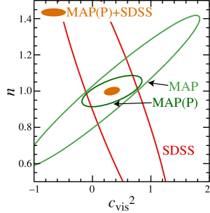
FIG. 2.: (left) The anisotropy spectrum of the $2K$ cosmic neutrino background. The small quadrupole, $\ell=2$, anisotropy in the neutrino background acts as a source of viscosity in the fluid. At early times when the neutrino energy density was higher than today, this viscosity altered the evolution of the gravitational potentials and hence the CMB anisotropy. (right) A possible future $1\sigma$ “detection” of the neutrino signal. The ellipses show expected $1\sigma$ error contours from the experiments listed. The $x$-axis is the viscosity speed of sound. The difference between $0$ and $1/3$ in $c_{\rm vis}^{2}$ is the signal of the $\ell=2$ anisotropy in the neutrino spectrum of the left panel.

In the left panel of Fig. 2 we show a calculation of the anisotropy spectrum, from Ref. [17]. The $y$-axis scale is $\Delta T/T\sim 10^{-5}$ as for the photons. In the right panel of Fig. 2 [18] we show a possible future $1\sigma$ “detection” of the fluctuations in the neutrino background inferred from a combination of large-scale structure and CMB data. Clearly this particular example is somewhat fanciful. The “detection” is extremely marginal and the assumptions going into the calculation quite optimistic. However considering how hard it is to do this detection any other way, it serves to illustrate the power of combinations of astrophysical measurements to constrain fine details of all the components making up the energy density of the universe.

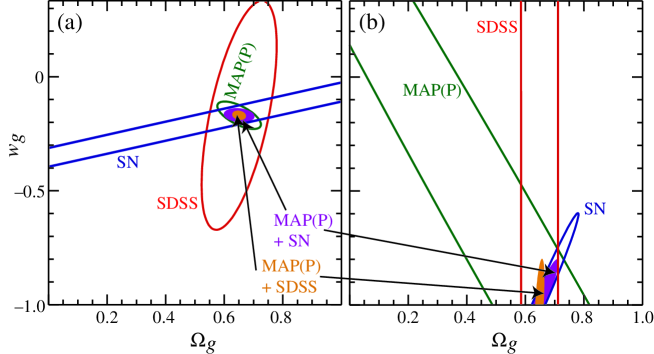
FIG. 3.: The expected $1\sigma$ contours on the equation of state $w=p/\rho$ and fraction of critical density $\Omega_{g}$ of a generalized dark energy candidate. Note that the errors do not depend strongly on the assumed equation of state. A model with $w_{g}=-1$ (right panel) is indistinguishable from a cosmological constant.

As another (topical) example, I show in Fig. 3 (also taken from Ref. [18]) the $1\sigma$ limits on the equation of state and fraction of critical density in “dark energy” such as a cosmological constant or dynamical scalar field (sometimes known as $x$CDM or quintessence). Note that regardless of the equation of state a $<10\%$ measurement of both the energy density and equation of state is possible.

These somewhat random examples should illustrate the power of the CMB to constrain cosmological parameters, under the assumption that our current models provide a good fit to the data. Of course it may always turn out that while the paradigm within which we are working is correct, our models are deficient in some detail which prevents a good fit to the data. The strategy in this case is to relax our assumptions and try to reconstruct the model from the observed spectrum. Perhaps eventually the missing ingredient can be found and utopia regained. In the meantime all is not lost.

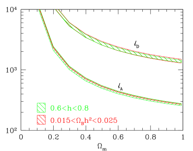
FIG. 4.: (left) The anisotropy spectrum for two different models of structure formation: an adiabatic model (solid line) and an isocurvature model (dashed line). Notice that the damping scale and the distance between the 2nd and 3rd peaks is model independent. (right) the dependence of the damping scale $\ell_{D}$ and the acoustic peak scale $\ell_{A}$ on the angular diameter distance back to $z\sim 10^{3}$. In this example, as the universe is made more open by lowering $\Omega_{m}$ without introducing a cosmological constant, the structure shifts to smaller scales or higher $\ell$.

There exist several model-independent measurements of the cosmological parameters [11]. As an example I show in Fig. 4 two different models of structure formation, both in a critical density universe. The models are chosen not to be good fits to the data, but to be very different from each other. In relativistic perturbation theory there are two kind of perturbations: adiabatic and isocurvature. Any fluctuation can be decomposed into these two basis modes. The solid line in the left panel of Fig. 4 is an example of a pure adiabatic model while the dashed line is an example of a pure isocurvature model. Note that while many things are different in these two models, there are two things that remain fixed. First the damping tail is at the same angular scale in both models ($\ell\sim 1500$). Secondly the separation between e.g. the 2nd and 3rd peaks is the same in both models. The first statement is easy to understand. The damping comes from photon diffusion during the time it takes the universe to recombine [19, 20, 21]. Perturbations on scales smaller than the photon diffusion scale are erased, leading to the damping of power at high-$\ell$. Clearly this process is independent of the source of the fluctuations. The second statement is also easy to understand. The photon-baryon fluid behaves like an oscillator with a natural frequency. Once the “bell” is struck it wants to ring at that natural frequency. Thus even though the driving forces in the adiabatic and isocurvature models are different, the “ringing” of the higher peaks proceeds at the same frequency. So the peak spacing is fixed.

While the peak spacing $\ell_{A}$ and the damping scale $\ell_{D}$ are (nearly) independent of the model of structure formation, they do depend on the cosmology. Specifically on the mapping between physical scales at the surface of last scattering ($z\sim 10^{3}$) and angles on the sky. They are thus probes of the angular diameter distance to last scattering, as shown in the right panel of Fig. 4 for the case of an open universe. More general constraints in the $\Omega_{m}-\Omega_{\Lambda}$ plane or the $\Omega_{g}-w$ plane can be found in [22, 18] respectively.

To turn the problem around one can look for tests of the model of structure formation independent of the cosmology. Our most succesful class of models is those with an early epoch of accelerated expansion, i.e. inflationary models. Since accelerated expansion requires a fluid with negative pressure, it is intimately related to quantum mechanical considerations (the inner space–outer space connection). One of the greatest triumphs of the inflationary idea is that it provides a source of small adiabatic fluctuations which can grow, through gravitational instability, to form the CMB anisotropies and large-scale structure that we observe today. How can we test this paradigm for the generation of primoridal fluctuations? Any model of fluctuations should produce all 3 modes of perturbations: scalar modes (density perturbations), vector modes (fluid vorticity) and tensor modes (gravitational waves). The vectors have no growing mode and so after a few expansion times they have decayed away, leaving scalar and tensor modes. The presence of vector modes would thus be evidence for fluctuation generation activity while the CMB anisotropy was being formed, i.e. not inflation. The mere presence of tensor modes does not however argue one way or the other.

In inflationary models based on a single, slow-rolling scalar field the scalar modes are enhanced over the tensor modes by a large factor which is related to the tensor spectral index (see Ref. [23] for a review). The relation becomes an inequality if more than one field is important. Unfortunately the tensor spectral index is quite hard to measure unless the tensor signal is large, and usually an additional (model dependent) relation to the scalar spectral index is assumed instead. It has been argued that if the inflationary idea is to find a home in modern high-energy physics theories, rather than in effective or “toy” models, then the tensor signal is quite likely to be small [24]. While our ignorance of physics above the electroweak scale makes it dangerous to take particle physics predictions as gospel in cosmology, the observational situation also argues against a large tensor signal [25]. In some sense this is good news: a generic mechanism would presumably make scalar, vector and tensor perturbations in roughly the same amounts leading to $T/S\simeq 1$ today (the vectors having decayed). Inflation on the other hand predicts that the scalar signal is enhanced, lowering $T/S$ from this naive prediction, as observations currently prefer.

Luckily CMB based tests of inflation exist which do not require a measurement of the tensor signal [12, 13]. They rely on the fact that the only known way to generate adiabatic fluctuations (i.e. fluctuations in the energy density or curvature of space) on cosmological scales today is to have a period of accelerated expansion [26, 27, 11], i.e. inflation. The key then is to test for the adiabaticity of the fluctuations, which can be done with broader features than detailed fitting to extract small signals. Plausibility arguments suggest that if a peak in the anisotropy spectrum is observed near $\ell\sim 200$, the fluctuations are adiabatic. Isocurvature models generically predict a peak shifted to higher $\ell$ [11, 13] (see Fig. 4). Further support for this inference could be gained by measuring the 2nd and 3rd peaks, though some loopholes still remain [11, 28, 29, 13]. The sharpest tests of the model [13] can be performed if information about the polarization of the CMB is obtained (as both MAP and Planck intend).

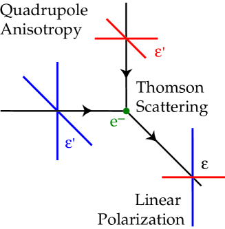
FIG. 5.: A quadrupole anisotropy at the surface of last scattering generates a linear polarization, since the angular dependence of Thomson scattering depends on the polarization of the ingoing and outgoing radiation.

Since $\gamma-e$ scattering depends on polarization and angle as $\epsilon_{f}\cdot\epsilon_{i}$, where $\epsilon_{f,i}$ are the polarization vectors of the final and inital radiation, a quadrupole anisotropy generates linear polarization (see Fig. 5). An introduction to polarization can be found in Ref. [30], and the numerous references therein. For our purposes here the key feature of polarization is that it is generated only by scattering. The small angle polarization is thus localized to the last-scattering surface, and provides us with a probe of the anisotropies (as a function of scale) at that time. The behaviour of the anisotropy around the horizon scale, and the slope of the spectrum at larger scales, then gives a test of the presence or absence of large-scale fluctuations in the curvature [31, 30].

In conclusion, cosmology is now in a “golden age”. We finally have the data to answer our most fundamental questions, and to generate new puzzles. Within a decade we hope to have a standard model of structure formation. Our current theoretical structure, starting with quantum fluctuations in the early universe, continuing with general relativistic dynamics and ending with free-fall of radiation and matter, is one of the most beautiful and complete in all of physics. Far from the cosmology of old, where order of magnitude estimates held sway, modern cosmology emphasizes precision calculations using well controlled approximations. The archetypical system of this “new era” is the microwave background. If our models are close to correct, high precision studies of the CMB anisotropy will revolutionize cosmology. If our models are wrong, one could not hope for a better data set with which to find the right path. We are all eagerly awaiting imminent experimental advances in this field.

REFERENCES

- [1] Smoot G., and Scott D., in “Review of Particle Properties”, p. 127, Caso C., et al., The European Physical Journal C3, 1 (1998).
- [2] Sachs R.K., Wolfe A.M., ApJ 147, 73 (1967).
- [3] White M., Hu W., Astron. & Astrophys. 321, 8 (1997) [astro-ph/9609105]
- [4] Lawrence C.R., Scott D., and White M., preprint [astro-ph/9810446]
- [5] Bennett C.L., Turner M.S., and White M., Phys. Today 50, 32 (1997).
- [6] Hu W., Sugiyama N., and Silk J., Nature 386, 37 (1997) [astro-ph/9604166]
- [7] Scott D., and White M., Gen. Rel. and Gravitation 27, 1023 (1995) [astro-ph/9505102]
- [8] White M., Scott D., and Silk J., Ann. Rev. Astron. Astrophys. 32, 319 (1994).
- [9] Hu W., Seljak U., White M., and Zaldarriaga M., Phys. Rev. D57, 3290 (1998) [astro-ph/9709066]
- [10] Eisenstein D.J., Hu W., and Tegmark M., [astro-ph/9807130]
- [11] Hu W., and White M., ApJ 471, 30 (1996) [astro-ph/9602019]
- [12] Hu W., and White M., Phys. Rev. Lett. 77, 1687 (1996) [astro-ph/9602020]
- [13] Hu W., Spergel D.N., and White M., Phys. Rev. D55, 3288 (1997) [astro-ph/9605193]
- [14] Hu W., ApJ 506, 485 (1998) [astro-ph/9801234]
- [15] Hu W., Eisenstein D.J., preprint [astro-ph/9809368]
- [16] Hu W., Eisenstein D.J., Tegmark M., Phys. Rev. Lett. 80, 5255 (1998) [astro-ph/9712057]
- [17] Hu W., Scott D., Sugiyama N., and White M., Phys. Rev. D52, 5498 (1995) [astro-ph/9505043]
- [18] Hu W., Eisenstein D.J., Tegmark M., and White M., Phys. Rev. D59, 023512 (1999) [astro-ph/9806362]
- [19] Silk J., ApJ 151, 459 (1969).
- [20] Efstathiou G., Bond J.R., MNRAS 227, 33 (1987)
- [21] Hu W., White M., ApJ 479, 568 (1997) [astro-ph/9609079]
- [22] White M., ApJ 506, 495 (1998) [astro-ph/9802295]
- [23] Lidsey J.E., et al., Rev. Mod. Phys. 69, 373 (1997) [astro-ph/9508078]
- [24] Lyth D., Phys. Rev. Lett. 78, 1861 (1997).
- [25] Zibin J., Scott D., White M., preprint [astro-ph/9901028]
- [26] Hu Y., Turner M.S., Weinberg E.J., Phys. Rev. D49, 3830 (1994)
- [27] Liddle A.R., Phys. Rev. D51, 5347 (1995)
- [28] Turok N., Phys. Rev. D54, 3686 (1996) [astro-ph/9604172]
- [29] Turok N., Phys. Rev. Lett. 77, 4138 (1996) [astro-ph/9607109]
- [30] Hu W., and White M., New Astronomy 2, 323 (1997) [astro-ph/9706147]
- [31] Hu W., and White M., Phys. Rev. D56, 596 (1997) [astro-ph/9702170]