The kinematics and the origin of the ionized gas in NGC 4036

Abstract

We present the kinematics and photometry of the stars and of the ionized gas near the centre of the S0 galaxy NGC4036. Dynamical models based on the Jeans Equation have been constructed from the stellar data to determine the gravitational potential in which the ionized gas is expected to orbit. Inside $10^{\prime\prime}$, the observed gas rotation curve falls well short of the predicted circular velocity. Over a comparable radial region the observed gas velocity dispersion is far higher than the one expected from thermal motions or small scale turbulence, corroborating that the gas cannot be following the streamlines of nearly closed orbits. We explore several avenues to understand the dynamical state of the gas: (1) We treat the gas as a collisionless ensemble of cloudlets and apply the Jeans Equation to it; this modeling shows that inside $4^{\prime\prime}$ the gas velocity dispersion is just high enough to explain quantitatively the absence of rotation. (2) Alternatively, we explore whether the gas may arise from the ‘just shed’ mass-loss envelopes of the bulge stars, in which case their kinematics should simply mimic that of the stars. he latter approach matches the data better than (1), but still fails to explain the low velocity dispersion and slow rotation velocity of the gas for $5^{\prime\prime}<r<10^{\prime\prime}$. (3) Finally, we explore, whether drag forces on the ionized gas may aid in explaining its peculiar kinematics. While all these approaches provide a much better description of the data than cold gas on closed orbits, we do not yet have a definitive model to describe the observed gas kinematics at all radii. We outline observational tests to understand the enigmatic nature of the ionized gas.

1 Introduction

Stars and ionized gas provide independent probes of the mass distribution in a galaxy. The comparison between their kinematics is particularly important in dynamically hot systems (i.e. whose projected velocity dispersion is comparable to rotation). In fact in elliptical galaxies and bulges the ambiguities about orbital anisotropies can lead to considerable uncertainties in the mass modeling (e.g. Binney & Mamon 1982; Rix et al. 1997).

The mass distributions inferred from stellar and gaseous kinematics are usually in good agreement for discs (where both tracers can be considered on nearly circular orbits), but often appear discrepant for bulges (e.g. Fillmore, Boroson & Dressler 1986; Kent 1988; Kormendy & Westpfahl 1989; Bertola et al. 1995b). There are several possibilities to explain these discrepant mass estimates in galactic bulges:

1. If bulges have a certain degree of triaxiality, depending on the viewing angle the gas on closed orbits can either move faster or slower than in the ‘corresponding’ axisymmetric case (Bertola, Rubin & Zeilinger 1989). Similarly, the predictions of the triaxial stellar models deviate from those in the axisymmetric case: whenever $\sigma_{\rm stars}>\sigma_{\rm axisym}$, then $v_{\rm stars}<v_{\rm axisym}$;

2. Most of the previous modeling assumes that the gas is dynamically cold and therefore rotates at the local circular speed on the galactic equatorial plane. If in bulges the gas velocity dispersion $\sigma_{\rm gas}$ is not negligible (e.g. Cinzano & van der Marel 1994 hereafter CvdM94; Rix et al. 1995; Bertola et al. 1995b), the gas rotates slower than the local circular velocity due to its dynamical pressure support. CvdM94 showed explicitly for the E4/S0a galaxy NGC 2974 that the gas and star kinematics agree taking into account for the gas velocity dispersion. Furthermore, if $\sigma_{\rm gas}$ is comparable to the observed streaming velocity, the spatial gas distribution can no longer be modeled as a disc;

3. Forces other than gravity (such as magnetic fields, interactions with stellar mass loss envelopes and the hot gas component) might act on the ionized gas (e.g. Mathews 1990).

In this paper we pursue the second of these explanations by building for NGC 4036 dynamical models which take into account both for the random motions and the three-dimensional spatial distribution of the ionized gas.

NGC 4036 has been classified S0₃(8)/Sa in RSA (Sandage & Tammann 1981) and S0^- in RC3 (de Vaucouleurs et al. 1991). It is a member of the LGG 266 group, together with NGC 4041, IC 758, UGC 7009 and UGC 7019 (Garcia 1993). It forms a wide pair with NGC 4041 with a separation of $17^{\prime}$ corresponding to 143 kpc at their mean redshift distance of 29 Mpc (Sandage & Bedke 1994). In The Carnegie Atlas of Galaxies (hereafter CAG) Sandage & Bedke (1994) describe it as characterized by an irregular pattern of dust lanes threaded through the disc in an ‘embryonic’ spiral pattern indicating a mixed S0/Sa form (see Panel 60 in CAG). Its total $V-$band apparent magnitude is $V_{T}=10.66$ mag (RC3). This corresponds to a total luminosity $L_{V}=4.2\cdot 10^{10}$ L${}_{\odot\,V}$ at the assumed distance of $d=30.2$ Mpc. The distance of NGC 4036 was derived as $d=V_{0}/H_{0}$ from the systemic velocity corrected for the motion of the Sun with respect to the centroid of the Local Group $V_{0}=1509\pm 50$ $\rm km\;s^{-1}$ (RSA) and assuming $H_{0}=50$ $\rm km\;s^{-1}\;Mpc^{-1}$. At this distance the scale is 146 pc arcsec^-1.

The total masses of neutral hydrogen and dust in NGC 4036 are $M_{\rm HI}=1.7\cdot 10^{9}$ M_⊙ and $M_{\rm dust}=4.4\cdot 10^{5}$ M_⊙ (Roberts et al. 1991). NGC 4036 is known to have emission lines from ionized gas (Bettoni & Buson 1987) and the mass of the ionized gas is $M_{\rm HII}=7\cdot 10^{4}$ M_⊙ (see Sec. 4.1 for a discussion).

This paper is organized as follows. In Sec. 2 we present the photometrical and spectroscopical observations of NGC 4036, the reduction of the data, and the analysis procedures to measure the surface photometry and the major-axis kinematics of stars and ionized gas. In Sec. 3 we describe the stellar dynamical model (based on Jeans Equations), and we find the potential due to the stellar bulge and disc components starting from the observed surface brightness of the galaxy. In Sec. 4 we use the derived potential to study the dynamics of both the gaseous spheroid and disc components, assumed to be composed of collisionless cloudlets orbiting as test particles. In Sec. 5 we discuss our conclusions.

2 Observations and data analysis

2.1 Photometrical observations

2.1.1 Ground-based data

We obtained an image of NGC 4036 of 300 s in the Johnson $V-$band at the 2.3-m Bok Telescope at Kitt Peak National Observatory on December 22, 1995.

A front illuminated 2048$\times$2048 LICK2 Loral CCD with $15\times 15~{}\mu$m² pixels was used as detector at the Richtey-Chretien focus, $f/9$. It yielded a flat field of view with a $10\aas@@fstack{\prime}1$ diameter. The image scale was $0\aas@@fstack{\prime\prime}43$ pixel^-1 after a $3\times 3$ pixel binning. The gain and the readout noise were 1.8 e^- ADU^-1 and 8 e^- respectively.

The data reduction was carried out using standard IRAF routines. The image was bias subtracted and then flat-field corrected. The cosmic rays were identified and removed. A Gaussian fit to field stars in the resulting image yielded a measurement of the seeing point spread function (PSF) FWHM of $1\aas@@fstack{\prime\prime}7$.

The sky subtraction and elliptical fitting of the galaxy isophotes were performed by means of the Astronomical Images Analysis Package (AIAP) developed at the Osservatorio Astronomico di Padova (Fasano 1990). The sky level was determined by a polynomial fit to the surface brightness of the frame regions not contaminated by the galaxy light, and then subtracted out from the total signal. The isophote fitting was performed masking the bad columns of the frame and the bright stars of the field. Particular care was taken in masking the dust-affected regions along the major axis between $5^{\prime\prime}$ and $20^{\prime\prime}$. No photometric standard stars were observed during the night. For this reason the absolute calibration was made scaling the total apparent $V-$band magnitude to $V_{\rm T}=10.66$ mag (RC3).

Fig. 1 shows the $V-$band surface brightness ($\mu_{V}$), ellipticity ($\epsilon$), major axis position angle (PA), and the $\cos 4\theta$ ($a_{4}$) Fourier coefficient of the isophote’s deviations from elliptical as functions of radius along the major axis.

Figure 1: Ground-based $V-$band observed surface-brightness, ellipticity, position angle and $\cos 4\theta$ coefficient radial profiles of NGC 4036. The dashed line in the top panel represents the surface-brightness profile of the exponential disc of the best-fit kinematical model ($\mu_{0}=19.3$ $\rm mag\;arcsec^{-2}$, $r_{d}=22\aas@@fstack{\prime\prime}0$ and $i=72\degr$) derived in Sec. 3.2.3.

For $r\la 4^{\prime\prime}$ the ellipticity is $\ga 0.12$. Between $r\sim 4^{\prime\prime}$ and $r\sim 30^{\prime\prime}$ it increases to $0.61$. It rises to $0.63$ at $r\sim 62^{\prime\prime}$ and then it decreases to $0.56$ at the farthest observed radius. The position angle ranges from $\sim 98\degr$ to $\sim 67\degr$ in the inner $5^{\prime\prime}$. Between $r\sim 5^{\prime\prime}$ and $r\sim 10^{\prime\prime}$ it increases to $\sim 79\degr$ and then it remains constant. The $\cos 4\theta$ coefficient ranges between $\sim+0.01$ and $\sim-0.02$ for $r\la 5^{\prime\prime}$. Further out it peaks to $\sim+0.05$ at $r\sim 18^{\prime\prime}$, and then it decreases to $\sim+0.03$ for $r>30^{\prime\prime}$. The abrupt variation in position angle ($\rm\Delta\,PA\,\simeq\,30\degr$) observed inside $5^{\prime\prime}$ leads to an isophote twist that can be interpreted as due to a slight triaxiality of the inner regions of the stellar bulge. Anyway this variation has to be considered carefully due to the presence of dust pattern in these regions which are revealed by HST imaging (see Fig. 2).

These results are consistent with previous photometric studies of Kent (1984) and Michard (1993) obtained in the $r-$ and $B-$band respectively. Our measurements of ellipticity follows closely those by Michard (1993). Kent (1984) measured the ellipticity and position angle of NGC 4036 isophotes in $r-$band for $9^{\prime\prime}\leq\,r\,\leq\,114^{\prime\prime}$. Out to $r=78^{\prime\prime}$ the $r-$band ellipticity is lower than our $V-$band one by $\sim 0.04$. The $r-$band position angle profile differs from our only at $r\sim 16^{\prime\prime}$ ($\epsilon_{r}=76\degr$) and for $r>78^{\prime\prime}$ ($\epsilon_{r}=81\degr$). We found $\cos 4\theta$ isophote deviation from ellipses to have a radial profile in agreement with that by Michard (1993).

2.1.2 Hubble Space Telescope data

In addition, we derived the ionized gas distribution in the nuclear regions of NGC 4036 by the analysis of two Wide Field Planetary Camera 2 (WFPC2) images which were extracted from the Hubble Space Telescope archive.

We used a 300 s image obtained on August 08, 1994 with the F547M filter (principal investigator: Sargent GO-05419) and a 700 s image taken on May 15, 1997 with the F658N filter (principal investigator: Malkan GO-06785).

The standard reduction and calibration of the images were performed at the STScI using the pipeline-WFPC2 specific calibration algorithms. Further processing using the IRAF STSDAS package involved the cosmic rays removal and the alignment of the images (which were taken with different position angles). The surface photometry of the F547M image was carried out using the STSDAS task ELLIPSE without masking the dust lanes. In Fig. 2 we plot the resulting ellipticity ($\epsilon$) and major axis position angle (PA) of the isophotes as functions of radius along the major axis.

Figure 2: Surface brigthness, ellipticity and position angle radial profiles of the nuclear regions of NGC 4036 obtained from a HST image (crosses) compared to the ground-based data before (filled squares) and after (open circles) the seeing deconvolution (see Sec. 3.2.1). The WFPC2 image is in the F547W$-$band while the ground-based ones are in the $V-$band.

The continuum-free image of NGC 4036 (Fig. 3) was obtained by subtracting the continuum-band F547M image suitably scaled, from the emission-band F658N image The mean scale factor for the continuum image was estimated by comparing the intensity of a number of 5$\times$5 pixels regions near the edges of the frames in the two bandpasses. These regions were chosen in the F658N image to be emission free. Our continuum-free image reveals that less than the $40\%$ of the H$\alpha$$\times$[N II] flux of NGC 4036 derives from a clumpy structure of about $6^{\prime\prime}\times 2^{\prime\prime}$. The center of this complex filamentary structure which is embedded in a smooth emission pattern coincides with the position of the maximum intensity of the continuum.

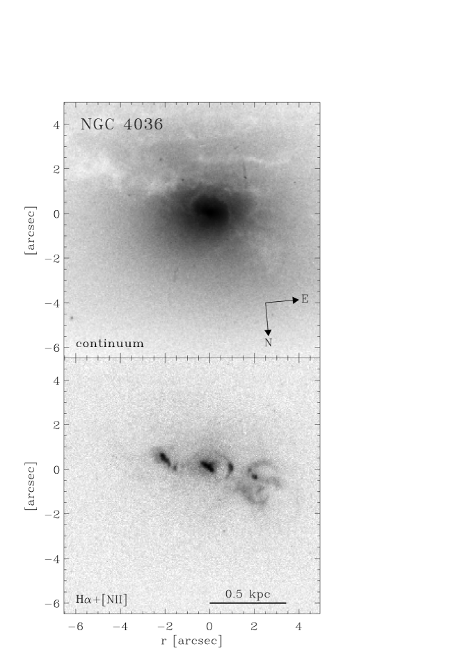
Figure 3: WFPC2 stellar continuum image (upper panel) and the continuum-subtracted H$\alpha$$+$[N II] emission image (lower panel) of the nucleus of NGC 4036.

2.2 Spectroscopical observations

A major-axis (PA$=85\degr$) spectrum of NGC 4036 was obtained on March 30, 1989 with the Red Channel Spectrograph at the Multiple Mirror Telescope as a part of a larger sample of 8 S0 galaxies (Bertola et al. 1995b).

The exposure time was 3600 s and the 1200 grooves mm^-1 grating was used in combination with a $1\aas@@fstack{\prime\prime}25\times 180^{\prime\prime}$ slit. It yielded a wavelength coverage of 550 Å between about 3650 Å and about 4300 Å with a reciprocal dispersion of 54.67 Å mm^-1. The spectral range includes stellar absorption features, such as the the Ca II H and K lines ($\lambda\lambda\,$3933.7, 3968.5 Å) and the Ca I g-band ($\lambda\,$4226.7 Å), and the ionized gas [O II] emission doublet ($\lambda\lambda\,$3726.2. 3728.9 Å). The instrumental resolution was derived measuring the $\sigma$ of a sample of single emission lines distributed all over the spectral range of a comparison spectrum after calibration. We checked that the measured $\sigma$’s did not depend on wavelength, and we found a mean value $\sigma=1.1$ Å. It corresponds to a velocity resolution of $\sim 88$ $\rm km\;s^{-1}$ at 3727 Å and $\sim 83$ $\rm km\;s^{-1}$ at 3975 Å. The adopted detector was the 800$\times$800 Texas Instruments CCD, which has 15$\times$15 $\mu$m² pixel size. No binning or rebinning was done. Therefore each pixel of the frame corresponds to $0.82$ Å $\times\ 0\aas@@fstack{\prime\prime}33$.

Some spectra of late-G and early-K giant stars were taken with the same instrumental setup for use as velocity and velocity dispersion templates in measuring the stellar kinematics. Comparison helium-argon lamp exposures were taken before and after every object integration. The seeing FWHM during the observing night was in between $1^{\prime\prime}$ and $1\aas@@fstack{\prime\prime}5$.

The data reduction was carried out with standard procedures from the ESO-MIDAS package. The spectra were bias subtracted, flat-field corrected, cleaned for cosmic rays and wavelength calibrated. The sky contribution in the spectra was determined from the edges of the frames and then subtracted.

2.2.1 Stellar kinematics

The stellar kinematics was analyzed with the Fourier Quotient Method (Sargent et al. 1977) as applied by Bertola et al. (1984). The K4III star HR 5201 was taken as template. It has a radial velocity of $-2.7$ $\rm km\;s^{-1}$ (Evans 1967) and a rotational velocity of 10 $\rm km\;s^{-1}$ (Bernacca & Perinotto 1970). No attempt was made to produce a master template by combining the spectra of different spectral types, as done by Rix & White (1992) and van der Marel et al. (1994). The template spectrum was averaged along the spatial direction to increase the signal-to-noise ratio ($S/N$). The galaxy spectrum was rebinned along the spatial direction until a ratio $S/N\geq 10$ was achieved at each radius. Then spectra of galaxy and template star were rebinned to a logarithmic wavelength scale, continuum subtracted and endmasked. The least-square fitting of Gaussian broadened spectrum of the template star to the galaxy spectrum was done in the Fourier space over the restricted range of wavenumbers $\left[k_{\it min},k_{\it max}\right]=\left[5,200\right]$. In this way we rejected the low-frequency trends (corresponding to $k<5$) due to the residuals of continuum subtraction and the high-frequency noise (corresponding to $k>200$) due to the instrumental resolution. (The wavenumber range is important in particular in the Fourier fitting of lines with non-Gaussian profiles, see van der Marel & Franx 1993; CvdM94).

The values obtained for the stellar radial velocity and velocity dispersion as a function of radius are given in Tab. 2. The table reports the galactocentric distance $r$ in arcsec (Col. 1), the heliocentric velocity $V$ (Col. 2) and its error $\delta V$ (Col. 3) in $\rm km\;s^{-1}$, the velocity dispersion $\sigma$ (Col. 4) and its error $\delta\sigma$ (Col. 5) in $\rm km\;s^{-1}$. The values for the stellar $\delta V$ and $\delta\sigma$ are the formal errors from the fit in the Fourier space.

The systemic velocity was subtracted from the observed heliocentric velocities and the profiles were folded about the centre, before plotting. We derive for the systemic heliocentric velocity a value $V_{\odot}=1420\pm 15$ $\rm km\;s^{-1}$. Our determination is in agreement within the errors with $V_{\odot}=1397\pm 27$ $\rm km\;s^{-1}$ (RC3) and $V_{\odot}=1382\pm 50$ $\rm km\;s^{-1}$ (RSA) derived from optical observations too. The resulting rotation curve, velocity dispersion profile and rms velocity ($\sqrt{v^{2}+\sigma^{2}}$) curve for the stellar component of NGC 4036 are shown in Fig. 4. The kinematical profiles are symmetric within the error bars with respect to the galaxy centre. For $r\la 2^{\prime\prime}$ the rotation velocity increases almost linearly with radius up to $\sim 100$ $\rm km\;s^{-1}$, remaining approximatively constant between $2^{\prime\prime}$ and $4^{\prime\prime}$. Outwards it rises to the farthest observed radius. It is $\sim 180$ $\rm km\;s^{-1}$ at $9^{\prime\prime}$, $\sim 220$ $\rm km\;s^{-1}$ at $21^{\prime\prime}$ and $\sim 260$ $\rm km\;s^{-1}$ at $29^{\prime\prime}$. The velocity dispersion $\sigma\sim 210$ $\rm km\;s^{-1}$ in the centre and at $r\sim 4^{\prime\prime}$ with a ‘local minimum of $\sim 180$ at $r=2^{\prime\prime}$. Further out it declines to values $\la 120$ $\rm km\;s^{-1}$.

Figure 4: Stellar kinematics along the major axis of NGC 4036. The folded rotation velocity curve (top panel), velocity dispersion profile (middle panel) and rms velocity curve (bottom panel) are shown in $\rm km\;s^{-1}$. Open squares and filled triangles represent data derived for the approaching W and receding E side respectively.

Figure 5: Ionized gas kinematics along the major axis of NGC 4036. The folded rotation velocity curve (top panel), velocity dispersion profile (middle panel) and rms velocity curve (bottom panel) are shown in $\rm km\;s^{-1}$. Open squares and filled triangles represent data derived for the approaching W and receding E side respectively. The velocity error bars indicate the formal error of double Gaussian fit to the [O II] doublet. The error bars in the velocity dispersions take also into account for the subtraction of the instrumental dispersion.

2.2.2 Ionized gas kinematics

To determine the ionized gas kinematics we studied the [O II] ($\lambda\lambda\,$3726.2, 3728.9 Å) emission doublet. In our spectrum the two lines are not resolved at any radius. We obtained smooth fits to the [O II] doublet using a two-steps procedure. In the first step the emission doublet was analyzed by fitting a double Gaussian to its line profile, fixing the ratio between the wavelengths of the two lines and assuming that both lines have the same dispersion. The intensity ratio of the two lines depends on the state (i.e. electron density and temperature) of the gas (e.g. Osterbrock 1989). We found a mean value of [O II]$\,\lambda 3726.2$/[O II]$\,\lambda 3728.9$$\,=0.8\pm 0.1$ without any significative dependence on radius. The electron density derived from the obtained intensity ratio of [O II] lines is in agreement with that derived (at any assumed electron temperature, see Osterbrock 1989) from the intensity ratio of the [S II] lines ([S II]$\,\lambda 6716.5$/[S II]$\,\lambda 6730.9$=1.23) found by Ho, Filippenko & Sargent (1997). In the second step we fitted the line profile of the emission doublet by fixing the intensity ratio of its two lines at the value above. At each radius we derived the position, the dispersion and the uncalibrated intensity of each [O II] emission line and their formal errors from the best-fitting double Gaussian to the doublet plus a polynomial to its surrounding continuum. The wavelength of the lines’ centre was converted into the radial velocity and then the heliocentric correction was applied. The lines’ dispersion was corrected for the instrumental dispersion and then converted into the velocity dispersion.

The measured kinematics for the gaseous component in NGC 4036 is given in Tab. 3. The table contains the galactocentric distance $r$ in arcsec (Col. 1), the heliocentric velocity $V$ (Col. 2) and its error $\delta V$ (Col. 3) in $\rm km\;s^{-1}$ the velocity dispersion $\sigma$ (Col. 4) and its errors $\delta\sigma_{+}$ and $\delta\sigma_{-}$ (Cols. 5 and 6) in $\rm km\;s^{-1}$. The gas velocity errors $\delta V$ are the formal errors for the double Gaussian fit to the [O II] doublet. The gas velocity dispersion errors $\delta\sigma_{+}$ and $\delta\sigma_{-}$ take also account for the subtraction of the instrumental dispersion.

The rotation curve, velocity dispersion profile and rms velocity curve for the ionized gas component of NGC 4036 resulting after folding about the centre are shown Fig. 5. The [O II]$\,\lambda 3726.2$ intensity profile as a function of radius is plotted in Fig. 6. The gas rotation tracks the stellar rotation remarkably well. They are consistent within the errors to one another. The gas velocity dispersion has central dip of $\sim 160$ $\rm km\;s^{-1}$ with a maximum of $\sim 220$ $\rm km\;s^{-1}$ at $r\sim 2^{\prime\prime}$. It remains higher than 100 $\rm km\;s^{-1}$ up to $\sim 4^{\prime\prime}$ before decreasing to lower values. The velocity dispersion profile appears to be less symmetric than the rotation curve. Indeed between $2^{\prime\prime}$ and $5^{\prime\prime}$ the velocity dispersion measured onto the E side rapidly drops from its observed maximum to $\sim 50$ $\rm km\;s^{-1}$, while in the W side it smoothly declines to $\sim 140$ $\rm km\;s^{-1}$. Errors on the gas velocity dispersion increase at large radii as the gas velocity dispersion becomes comparable to the instrumental dispersion.

Figure 6: The intensity of the [O II]$\,\lambda 3726.2$ line as function of radius in NGC 4036. Since the spectrum was not flux calibrated the scale has an arbitrary zero point. The thick continuous lines connect the measurements along the W and E side respectively. The vertical bar on the left-hand side of the panel represents the typical error for the data. The dashed and dotted lines represent respectively the profile of the gaseous $R^{1/4}$ spheroid and gaseous exponential disc derived in Sec. 4.1. The thin continuous line is the fit to the data.

2.2.3 Comparison with kinematical data by Fisher (1997)

The major-axis kinematics for stars and gas we derived for NGC 4036 are consistent within the errors with the measurements of Fisher (1997, hereafter F97). The only exception is represented by the differences of $20\%$–$30\%$ between our and F97 stellar velocity dispersions in the central $8^{\prime\prime}$. In these regions F97 finds a flat velocity dispersion profile with a plateau at $\sigma\sim 170$ $\rm km\;s^{-1}$. To measure stellar kinematics he adopted the Fourier Fitting Method (van der Marel & Franx 1993) directly on the line-of-sight velocity distribution derived with Unresolved Gaussian Decomposition Method (Kuijken & Merrifield 1993). For $|r|\la 8^{\prime\prime}$ the NGC 4036 line profiles are asymmetric (displaying a tail opposite to the direction of rotation) and flat-toped, as result from the $h_{3}$ and $h_{4}$ radial profiles. The $h_{3}$ and $h_{4}$ parameters measure respectively the asymmetric and symmetric deviations of the line profile from a Gaussian (van der Marel & Franx 1993; Gerhard 1993). For NGC 4036 the $h_{3}$ term anticorrelates with $v$, rising to $\sim+0.1$ in the approaching side and falling to $\sim-0.1$ in the receding side. The $h_{4}$ term exhibits a negative value ($\sim-0.03$).

3 Modeling the stellar kinematics

3.1 Modeling technique

We built an axisymmetric bulge-disc dynamical model for NGC 4036 applying the Jeans modeling technique introduced by Binney, Davies & Illingworth (1990), developed by van der Marel, Binney & Davies (1990) and van der Marel (1991), and extended to two-component galaxies by CvdM94 and to galaxies with a DM halo by Cinzano (1995) and Corsini et al. (1998). For details the reader is referred the above references.

The main steps of the adopted modeling are (i) the calculation of the bulge and disc contribution to the potential from the observed surface brightness of NGC 4036; (ii) the solution of the Jeans Equations to obtain separately the bulge and disc dynamics in the total potential; and (iii) the projection of the derived dynamical quantities onto the sky-plane taking into account seeing effects, instrumental set-up and reduction technique to compare the model predictions with the measured stellar kinematics. In the following each invidual step is briefly discussed:

1. We model NGC 4036 with an infinitesimally thin exponential disc in its equatorial plane. The disc surface mass density is specified for any inclination $i$, central surface brightness $\mu_{0}$, scale length $r_{d}$ and constant mass-to-light ratio $(M/L)_{d}$. The disc potential is calculated from the surface mass density as in Binney & Tremaine (1987). The limited extension of our kinematical data (measured out $r<30^{\prime\prime}\,\simeq\,0.5\,R_{\it opt}$) prevents us to disentangle in the assumed constant mass-to-light ratios the possible contribution of a dark matter halo.
   The surface brightness of the bulge is obtained by subtracting the disc contribution from the total observed surface brightness. The three-dimensional luminosity density of the bulge is obtained deprojecting its surface brightness with an iterative method based on the Richardson-Lucy algorithm (Richardson 1972; Lucy 1974). Its three-dimensional mass density is derived by assuming a constant mass-to-light ratio $(M/L)_{b}$. The potential of the bulge is derived solving the Poisson Equation by a multipole expansion (e.g. Binney & Tremaine 1987).

2. The bulge and disc dynamics are derived by separately solving the Jeans Equations for each component in the total potential of the galaxy. For both components we assume a two integral distribution function of the form $f=f(E,L_{z})$. It implies that the vertical velocity dispersion $\sigma^{2}_{z}$ is equal to second radial velocity moment $\sigma_{R}^{2}$ and that $\overline{v_{R}v_{z}}=0$. Therefore the Jeans Equations becomes a closed set, which can be solved for the unknowns $\overline{v^{2}_{\phi}}$ and $\sigma^{2}_{R}=\sigma^{2}_{z}$. Other assumptions to close the Jeans Equations are also possible (e.g. van der Marel & Cinzano 1992).
   For the bulge we made the same hypotheses of Binney et al. (1990). A portion of the second velocity moment $\overline{v^{2}_{\phi}}$ is assigned to bulge streaming velocity $\overline{v_{\phi}}$ following Satoh’s (1980) prescription.
   For the disc we made the same hypotheses of Rix & White (1992) and CvdM94. The second radial velocity moment $\sigma^{2}_{R}$ in the disc is assumed to fall off exponentially with a scale length $R_{\sigma}$ from a central value of $\sigma^{2}_{d0}$. The azimuthal velocity dispersion $\sigma^{2}_{\phi}$ in the disc is assumed to be related to $\sigma^{2}_{R}$ according to the relation from epicyclic theory [cfr. Eq. (3-76) of Binney & Tremaine (1987)]. As pointed out by CvdM94 this relation may introduce systematic errors (Kuijken & Tremaine 1992; Evans & Collett 1993; Cuddeford & Binney 1994). The disc streaming velocity $\overline{v_{\phi}}$ (i.e. the circular velocity corrected for the asymmetric drift) is determined by the Jeans equation for radial equilibrium.

3. We projected back onto the plane of the sky (at the given inclination angle) the dynamical quantities of both the bulge and the disc to find the line-of-sight projected streaming velocity and velocity dispersion. We assumed that both the bulge and disc have a Gaussian line profile. At each radius their sum (normalized to the relative surface brightness of the two components) represents the model-predicted line profile. As in CvdM94 the predicted line profiles were convolved with the seeing PSF of the spectroscopic observations and sampled over the slit width and pixel size to mimic the observational spectroscopic setup. We mimicked the Fourier Quotient method for measuring the stellar kinematics fitting the predicted line profiles with a Gaussian in the Fourier space to derive the line-of-sight velocities and velocity dispersions for the comparison with the observed kinematics. The problems of comparing the true velocity moments with the Fourier Quotient results were discussed by van der Marel & Franx (1993) and by CvdM94.

3.2 Results for the stellar component

3.2.1 Seeing-deconvolution

The modeling technique described in Sec. 3.1 derives the three-dimensional mass distribution from the three-dimensional luminosity distribution inferred from the observed surface photometry by a fine-tuning of the disc parameters leading to the best fit on the kinematical data. We performed a seeing-deconvolution of the $V-$band image of NGC 4036 to take into account the seeing effects on the measured photometrical quantities (surface-brightness, ellipticity and $\cos 4\theta$ deviation profiles) used in the deprojection of the two-dimensional luminosity distribution. We obtained a restored NGC 4036 image through an iterative method based on the Richardson-Lucy algorithm (Richardson 1972; Lucy 1974) available in the IRAF package STSDAS. We assumed the seeing PSF to be a circular Gaussian with a FWHM$=1\aas@@fstack{\prime\prime}7$. Noise amplification represents a main backdraw in all Richardson-Lucy iterative algorithms and the number of iterations needed to get a good image restoration depends on the steepness of the surface-brightness profile (e.g. White 1994). After 6 iterations, we did not notice any more substantial change in the NGC 4036 surface-brightness profile while the image became too noisy. Therefore we decided to stop at the sixth iteration. The surface-brightness, ellipticity, position angle radial profiles of NGC 4036 after the seeing-deconvolution are displayed in Fig. 2 compared with the HST and the unconvolved ground-based photometry. The raises found at small radii for the surface brightness ($r\sim 0.2$ $\rm mag\;arcsec^{-2}$) and for the ellipticity ($r\sim 0.05$) are comparable in size to the values found by Peletier et al. (1990) for seeing effects in the centre of ellipticals.

3.2.2 Bulge-disc decomposition

We performed a standard bulge-disc decomposition with a parametric fit (e.g. Kent 1985) in order to find a starting guess for the exponential disc parameters to be used in the kinematical fit. We decomposed the seeing-deconvolved surface-brightness profile on both the major and the minor axis as the sum of an $R^{1/4}$ bulge, having surface-brightness profile

$$\mu_{b}(r)=\mu_{e}+8.3268\left[\left(\frac{r}{r_{e}}\right)^{1/4}-1\right]\,,$$ (1)

plus an exponential disc, having surface-brightness profile

$$\mu_{d}(r)=\mu_{0}+1.0857\left(\frac{r}{r_{d}}\right)\,.$$ (2)

We assumed that the minor-axis profile of each component is the same as the major-axis profile, but scaled by a factor $1-\epsilon=b/a$. A least-squares fit of the photometric data provides $\mu_{e}$, $r_{e}$ and $\epsilon$ of the bulge, $\mu_{0}$, $r_{d}$ of the disc, and the galaxy inclination $i$ (see Tab. 1 for the results).

Kent (1984) measured surface photometry of NGC 4036 in the $r-$band. He decomposed the major- and minor-axis profiles in an $R^{1/4}$ bulge and in an exponential disc (Kent 1985). A rough but useful comparison between the bulge and disc parameters resulting from the two photometric decompositions is possible by a transformation from $r$- to $V-$band of Kent’s data. We derived from Kent’s surface brightness profile along the major axis of NGC 4036 its (extrapolated) total magnitude $r_{T}=10.56\pm 0.02$ corresponding to $V_{T}-r_{T}=0.13\pm 0.11$. Then we converted the $\mu_{0}$ and $\mu_{e}$ values from the $r$- to the $V-$band (see Tab. 1). The differences between the best-fit parameters obtained from the two decompositions are lower than $10\%$ except for bulge ellipticity (our value is $\sim 64\%$ than the Kent’s one). These discrepancies are consistent with the differences in the slope of the two surface-brightness profiles, with differences between the Kent’s approach to correct for the seeing effects [Kent (1985) convolved the theoretical bulge and disc profiles with the observed Gaussian seeing profile] and with the uncertainties of the conversion from $r$- to $V-$band of Kent’s surface brightnesses.

Table 1: The bulge-disc decomposition parameters

	bulge			disc
	$\mu_{e}$	$r_{e}$	$\epsilon$	$\mu_{0}$	$r_{d}$	$i$
this paper	20.4	$12\aas@@fstack{\prime\prime}8$	0.11	18.7	$22\aas@@fstack{\prime\prime}1$	$74\aas@@fstack{\circ}9$
Kent (1985)	20.7	$13\aas@@fstack{\prime\prime}1$	0.07	18.6	$21\aas@@fstack{\prime\prime}0$	$71\aas@@fstack{\circ}9$

Note. $\mu_{e}$ and $\mu_{0}$ are given in $V-$$\rm mag\;arcsec^{-2}$. Kent’s (1984) surface brightnesses have been converted from the $r$- to the $V-$band.

3.2.3 Modeling results

We looked for the disc parameters leading to the best fit of the observed stellar kinematics, using as starting guess those resulting from our best-fit photometric decomposition, with $|\mu_{0}-1|\leq 18.7$ $\rm mag\;arcsec^{-2}$, $|r_{d}-5^{\prime\prime}|\leq 22\aas@@fstack{\prime\prime}1$, and $|i-5\degr|\leq 74\aas@@fstack{\circ}9$. For any exponential disc of fixed $\mu_{0},r_{d},i$ (in the investigated range of values), we subtracted its surface brightness from the total seeing-deconvolved surface brightness. The residuum surface brightness was considered to be contributed by the bulge. Being $\mu_{0}$, $r_{d}$ and $i$ correlated, a bulge component with a surface-brightness profile consistent with that resulting from the photometric decomposition, was obtained only by taking exponential discs characterized by large $\mu_{0}$ values in combination with large values of $r_{d}$ (i.e. larger but fainter discs) or by small $\mu_{0}$ and small $r_{d}$ (i.e. smaller but brighter discs). After subtracting the disc contribution to the total surface brightness, the three-dimensional luminosity density of the bulge has been obtained after seven Richardson-Lucy iterations starting from a fit to the actual bulge surface brightness with the projection of a flattened Jaffe profile (1983). The residual surface brightness ($\Delta\mu=\mu_{\rm model}-\mu_{\rm obs}$) after each iteration and the final three-dimensional luminosity density profiles of the spheroidal component of NGC 4036 along the major, the minor and two intermediate axis is plotted for the kinematical best-fit model in Fig. 7 up to $100^{\prime\prime}$ (the stellar and ionized-gas kinematics are measured to $\sim 30^{\prime\prime}$).

Figure 7: The deprojection of the surface brightness of the spheroidal component of NGC 4036 for the best-fit kinematical model. The right panel shows the residual surface brightness $\Delta\mu$ in $\rm mag\;arcsec^{-2}$ after each Lucy iteration (dashed lines) from an initial Jaffe fit to the actual NGC 4036 bulge brightness. The residuals are shown for four axes (major through minor axis: top through bottom). For each set of curves: the solid line corresponds to the projected adopted model for the 3-D luminosity density and the dotted line corresponds to a perfect deprojection. At each interaction if the model is brighter than the galaxy, the corresponding dashed or continuous curve is below the dotted line. In the left panel the final three-dimensional luminosity density profile of the spheroidal component of NGC 4036 right panel is given in units of $10^{10}{\rm L_{\odot}\;kpc^{-3}}$ for the same four axes (minor through major axis: innermost through outermost curve).

We applied the modeling technique described in Sec. 3.1 considering only models in which the bulge is an oblate isotropic rotator (i.e. $k=1$) and in which the bulge and the disc have the same mass-to-light ratio $(M/L)_{b}=(M/L)_{d}$. The $M/L$ determines the velocity normalization and was chosen (for each combination of disc parameters) to optimize the fit to the rms velocity profile. The best-fit model to the observed major-axis stellar kinematics is obtained with a mass-to-light ratio $M/L_{V}$$=3.42$ M_⊙/L${}_{\odot\,V}$ and with an exponential disc having a surface-brightness profile

$$\mu_{d}(r)=19.3+1.0857\left(\frac{r}{22\aas@@fstack{\prime\prime}0}\right)\;{\rm mag\;arcsec}^{-2},$$ (3)

(represented by the dashed line in the upper panel of Fig. 1), a radial velocity dispersion profile

$$\sigma_{R}(r)=155\;e^{-r/27\aas@@fstack{\prime\prime}4}\;{\rm km\;s}^{-1},$$ (4)

(where the galactocentric distance $r$ is expressed in arcsec) and an inclination $i=72\degr$. Fig. 8 shows the comparison between the rotation curve, the dispersion velocity profile and the rms velocity curve predicted by the best-fit model (solid lines) with the observed stellar kinematics along the major axis of NGC 4036. The agreement is good.

Figure 8: Comparison of the model predictions to the stellar major-axis kinematic for NGC 4036. Data points are as in Fig. 4. The solid curves represent the velocity (upper panel), velocity dispersion (middle panel) and rms velocity (lower panel) radial profiles of the best-fit model (in which the disc parameters are $\mu_{0}=19.3$ $\rm mag\;arcsec^{-2}$, $r_{d}=22\aas@@fstack{\prime\prime}0$ and $i=72\degr$).

The derived $V-$band luminosities for bulge and disc are $L_{b}=2.8\cdot 10^{10}$ L${}_{\odot\,V}$ and $L_{d}=1.4\cdot 10^{10}$ L${}_{\odot\,V}$. They correspond to the masses $M_{b}=9.8\cdot 10^{10}$ M_⊙ and $M_{d}=4.8\cdot 10^{10}$ M_⊙. The total mass of the galaxy (bulge$+$disc) is $M_{T}=14.5\cdot 10^{10}$ M_⊙. The disc-to-bulge and disc-to-total $V-$band luminosity ratios are $L_{b}/L_{d}=0.58$ and $L_{d}/L_{T}=0.36$. The disc-to-total luminosity ratio as function of the galactocentric distance is plotted in Fig. 9.

Figure 9: Radial profile of the fraction of the light contributed by the stellar disc along the major axis of NGC 4036 as obtained by the best-fit model. The distance from the center is expressed in arcsec.

3.2.4 Uncertainty ranges for the disc parameters

The uncertainty ranges for the disc parameters are $19.1\la\mu_{0}\la 19.5$ $\rm mag\;arcsec^{-2}$, $20^{\prime\prime}\la r_{d}\la 24^{\prime\prime}$ and $71\degr\la i\la 73\degr$. In Fig. 10 the continuous and the dotted line show the kinematical profiles predicted for two discs with the same inclination ($i=72\degr$) and the same total luminosity of the best-fit disc but with a smaller ($\mu_{0}=19.1$ $\rm mag\;arcsec^{-2}$, $r_{d}=20\aas@@fstack{\prime\prime}0$) or greater ($\mu_{0}=19.5$ $\rm mag\;arcsec^{-2}$, $r_{d}=24\aas@@fstack{\prime\prime}0$) scale length respectively. In Fig. 11 the continuous and the dotted lines correspond to two discs with the same scale length ($r_{d}=22\aas@@fstack{\prime\prime}0$) of the best-fit disc but with a lower ($\mu_{0}=19.2$ $\rm mag\;arcsec^{-2}$, $i=71\degr$) or a higher ($\mu_{0}=19.4$ $\rm mag\;arcsec^{-2}$, $i=73\degr$) inclination. Their total luminosity is respectively $\sim 14\%$ lower and $\sim 16\%$ higher then that of the best-fit disc. The fit of these models to the data are also acceptable so we estimate a $\sim 15\%$ error in the determination of the disc luminosity and mass. The good agreement with observations obtained with $k=1$, $(M/L)_{b}=(M/L)_{d}$, and without a dark matter halo causes us to not investigate models with $k\neq 1$, $(M/L)_{b}\neq(M/L)_{d}$ or with radially increasing mass-to-light ratios. Therefore we cannot exclude them at all.

Figure 10: As in Fig. 8 but for a disc with $\mu_{0}=19.1$ $\rm mag\;arcsec^{-2}$, $r_{d}=20\aas@@fstack{\prime\prime}0$ and $i=72\degr$ (continuous line) and for a disc with $\mu_{0}=19.5$ $\rm mag\;arcsec^{-2}$, $r_{d}=24\aas@@fstack{\prime\prime}0$ and $i=72\degr$ (dotted line).

Figure 11: As in Fig. 8 but for a disc with $\mu_{0}=19.2$ $\rm mag\;arcsec^{-2}$, $r_{d}=22\aas@@fstack{\prime\prime}0$ and $i=71\degr$ (continuous line) and for a disc with $\mu_{0}=19.4$ $\rm mag\;arcsec^{-2}$, $r_{d}=22\aas@@fstack{\prime\prime}0$ and $i=73\degr$ (dotted line).

The $V-$band luminosity (after inclination correction) of the exponential disc corresponding to the model best-fit to the observed stellar kinematics is $\sim 75\%$ than that of the disc obtained from the parametric fit of the surface-brightness profiles. The differences between the disc parameters derived from NGC 4036 photometry ($\mu_{0}=18.7$ $\rm mag\;arcsec^{-2}$, $r_{d}=22\aas@@fstack{\prime\prime}1$, $i=74\aas@@fstack{\circ}9$) and from the stellar kinematics ($\mu_{0}=19.3$ $\rm mag\;arcsec^{-2}$, $r_{d}=22\aas@@fstack{\prime\prime}0$, $i=72\degr$) are expected. In fitting the NGC 4036 surface-brightness profiles the bulge is assumed (i) to be axisymmetric; (ii) to have a $R^{1/4}$ profile; (iii) and constant axial ratio (i.e. its isodensity luminosity spheroids are similar concentric ellipsoids). We adopted this kind of representation for the bulge component only to find rough bounds on the exponential disc parameters to be used in the kinematical fit. Often bulges have neither an $R^{1/4}$ law profile (e.g. Burstein 1979; Simien & Michard 1984) neither perfectly elliptical isophotes (e.g. Scorza & Bender 1990). Therefore in modeling the stellar kinematics the three-dimensional luminosity density $j_{b}$ of the stellar bulge is assumed (i) to be oblate axisymmetric; but (ii) not to be parametrized by any analytical expression; (iii) nor to have isodensity luminosity spheroids with constant axial ratio. The flattening of the spheroids increases with the galactocentric distance, as it appears from the three-dimensional luminosity density profiles plotted in Fig. 7 along different axes onto the meridional plane of NGC 4036. This flattening produces an increasing of the streaming motions for the bulge component assumed to be an isotropic rotator.

3.2.5 Modeling results with stellar kinematics by Fisher (1997)

The bulge and disc parameters found for our best-fit model reproduce also the major-axis stellar kinematics by F97. Rather than choosing an ‘ad hoc’ wavenumber range to emulate F97 analysis technique the fit to the predicted line profile was done in ordinary space and not in the Fourier space as done to reproduce our Fourier Quotient measurements. The good agreement of the resulting kinematical profiles with F97 measurements are shown in Fig. 12.

Figure 12: Comparison between the predictions of the same model of Fig. 8 with the stellar major-axis kinematics for NGC 4036 by Fisher (1997). Data points are as in Fig. 4. The solid curves represent the velocity $v$, velocity dispersion $\sigma$, $h_{3}$ and $h_{4}$ radial profiles of the best-fit model taking into account for Fisher’s data reduction technique.

4 Modeling of the ionized gas kinematics

4.1 Modeling technique

At small radii both the ionized gas velocity and velocity dispersion are comparable to the stellar values, for $r\leq 9^{\prime\prime}$ and $r\leq 5^{\prime\prime}$ respectively. This prevented us to model the ionized gas kinematics by assuming the gas had settled into a disc component as done by CvdM94 for NGC 2974. Moreover a change in the slope of the [O II]$\,\lambda 3726.2$ intensity radial profile (Fig. 6) is observed at $r\la 8^{\prime\prime}$, its gradient appears to be somewhat steeper towards the centre. The velocity dispersion and intensity profiles of the ionized gas suggest that it is distributed into two components (see also the distinct central structure in HST H$\alpha$$+$[N II] image, Fig. 3): a small inner spheroidal component and a disc.

We built a dynamical model for the ionized gas with a dynamically hot spheroidal and in a dynamically colder disc component.

The total mass of the ionized gas $M_{\rm HII}$ is negligible and the total potential is set only by the stellar component. The mass of the ionized gas can be derived from optical recombination line theory (see Osterbrock 1989) by the H$\alpha$ luminosity. For a given electron temperature $T_{\rm e}$ and density $N_{\rm e}$, the H II mass is given by

$$M_{\rm HII}=\left(L_{\rm H\alpha}m_{\rm H}/N_{\rm e}\right)/\left(4\pi j_{\rm H\alpha}/N_{\rm e}N_{\rm p}\right)$$ (5)

where $L_{\rm H\alpha}$ is the H$\alpha$ luminosity, $m_{\rm H}$ is the mass of the hydrogen atom, $j_{\rm H\alpha}$ is the H$\alpha$ emissivity, and $N_{\rm p}$ are the proton density (Tohline & Osterbrock 1976). The H$\alpha$ luminosity of NGC 4036 scaled to the adopted distance is $L_{\rm H\alpha}$$\,=5.6\cdot 10^{39}$ L_⊙ (Ho et al. 1997). The term $4\pi j_{\rm H\alpha}/N_{\rm e}N_{\rm p}$ is insensitive to changes of $N_{\rm e}$ over the range $10^{2}$ – $10^{6}$ cm^-3. It decreases by a factor 3 for changes of $T_{\rm e}$ over the range $5\cdot 10^{3}\,\degr$K – $2\cdot 10^{4}\,\degr$K (Osterbrock 1989). For an assumed temperature $T_{\rm e}=10^{4}\,\degr$K, the electron density is estimated to be $N_{\rm e}=2\cdot 10^{2}$ cm^-3 from the [S II] ratio found by Ho et al. (1997) implying $M_{\rm HII}=7\cdot 10^{4}$ M_⊙.

For the gaseous spheroid and disc we made two different sets of assumptions based on two different physical scenarios for the gas cloudlets.

4.1.1 Long-lived gas cloudlets (model A)

In a first set of models we described the gaseous component by a set of collisionless cloudlets in hydrostatic equilibrium. The small gaseous ‘spheroid’ is characterized by a density distribution and flattening different from those of stars. Its major-axis luminosity profile was assumed to follow an $R^{1/4}$ law. Adopting for it the Ryden’s (1992) analytical approximation, we obtained the three-dimensional luminosity density of the gaseous spheroid. The flattening of the spheroids $q$ was kept as free parameter. To derive the kinematics of the gaseous spheroid we solved the Jeans Equations under the same assumptions made in Sec. 3 for the stellar spheroid. In particular the streaming velocity $\overline{v_{\phi}}$ of gaseous bulge is derived from the second azimuthal velocity moment $\overline{v_{\phi}^{2}}$ using Satoh’s (1980) relation. For the ionized gaseous disc we solved the Jeans Equations under similar assumptions made in Sec. 3 for the stellar disc. Specifically, we assumed that the gaseous disc (i) has an exponential luminosity profile; (ii) is infinitesimally thin; (iii) has an exponentially decreasing $\sigma^{2}_{R}$; (iv) has $\sigma^{2}_{z}=\sigma^{2}_{R}$; (v) has $\sigma^{2}_{\phi}$ satisfying the epicyclic relation.

4.1.2 Gas cloudlets ‘just’ shed by the stars (model B)

In a second set of models we assumed that the emission observed in the gaseous spheroid and disc arise from material that was recently shed from stars. Different authors (Bertola et al. 1984; Fillmore et al. 1986; Kormendy & Westpfahl 1989; Mathews 1990) suggested that the gas lost (e.g. in planetary nebulae) by stars was heated by shocks to the virial temperature of the galaxy within $10^{4}$ years, a time shorter than the typical dynamical time of the galaxy. Hence in this picture the ionized gas and the stars have the same true kinematics, while their observed kinematics are different due to the line-of-sight integration of their different spatial distribution. Differences between the radial profiles of the gas emissivity and the stellar luminosity may be explained if both the gas emission process and the efficiency of the thermalization process show a variation with the galactocentric distance. The three-dimensional luminosity density of the spheroid is derived as in model A and the luminosity density profile of the disc is assumed to be exponential.

In both cases, the kinematics of the gaseous spheroid and disc were projected on the sky-plane to be compared to the observed ionized gas kinematics. Assuming a Gaussian line profile for both the gaseous components we derived the total line profile (which depends on the relative flux of the two components). As for the stellar components, we convolved the line profiles obtained for the ionized gas with the seeing PSF and we sampled them over the slit-width and pixel size to mimic the observational setup. This procedure is particularly important for the modeling of the observed kinematics near the centre. As a last step (in mimicking the measuring technique of the gaseous kinematics) we fitted a single Gaussian to the resulting line profile, after taking into account for the instrumental line profile.

4.2 Results for the gaseous component

We decomposed the [O II]$\,\lambda 3726.2$ intensity profile as the sum of an $R^{1/4}$ gaseous spheroid and an exponential gaseous disc. A least-squares fit of the observed data was done for $r>3^{\prime\prime}$ to deal with seeing effects (Fig. 6). The gas spheroid resulted to be the dominating component up to $r\sim 8^{\prime\prime}$ beyond the bright emission in Fig. 3. We derived the effective radius of the gaseous spheroid $r_{e,\,{\rm gas}}=0\aas@@fstack{\prime\prime}5\pm 0\aas@@fstack{\prime\prime}1$, the scale length of the gaseous disc $r_{d,\,{\rm gas}}=29\aas@@fstack{\prime\prime}8\pm 0\aas@@fstack{\prime\prime}9$, and the ratio between the effective intensity of the spheroid and the central intensity of the disc $I_{e,\,{\rm gas}}/I_{0,\,{\rm gas}}=718_{-153}^{+813}$. The uncertainties on the resulting parameters have been estimated by a separate decomposition on each side of the galaxy. With these parameters we applied the models for the gas kinematics described in Sec. 4.1.

Since in both models A and B the stellar density radial profile differs from the gas emissivity radial profile, it is interesting to check what is the relation between the three-dimensional stellar density $\rho_{\rm star}(R)$ and the three-dimensional gas emissivity $\nu_{\rm gas}(R)$. After deprojection we find they are related by the following relation

$$\nu_{\rm gas}(R)\propto\rho_{\rm star}^{2.3}(R)$$ (6)

in the range of galactocentric distances between $r\sim 2^{\prime\prime}$ and $r\sim 10^{\prime\prime}$. In a fully ionized gas the recombination rate is proportional to the square of the gas density (e.g., Osterbrock 1989), this is a power-law relation quite similar to Eq. 6.

For models A and B the best-fit to the observed gas kinematics are in both cases obtained with a spheroid flattening $q=0.8$, and are plotted respectively in Fig. 13 and Fig. 14.
The best result is obtained with model B. A simple estimate of the errors on the model due to the uncertainties of bulge-disc decomposition of the radial profile of [O II]$\,\lambda 3726.2$ emission line can be inferred by comparing the model predictions based on the separate decomposition on each side of the galaxy. We find a maximum difference of $5\%$ for $4^{\prime\prime}<r<10^{\prime\prime}$ between the gas velocities and velocity dispersion predicted using the two different bulge-disc decompositions of the [O II]$\,\lambda 3726.2$ intensity profile. For model A the assumption of Satoh’s (1980) relation fails in reproducing the observed gas kinematics for $r\la 6^{\prime\prime}$, where the emission lines intensity profile is dominated by the gaseous spheroidal component. However the $R^{1/4}$ extrapolation of the density profile in the inner $3^{\prime\prime}$ overestimates the density gradient in this region (as it appears also from the HST image, Fig. 3) which could produce an exceeding asymmetric drift correction.

Figure 13: Comparison of the predictions of model A (dashed curve) to the ionized gas kinematics observed along the major axis of NGC 4036. The data points are as in Fig. 5. The dotted curves represent the seeing-convolved circular velocity curve and zero velocity-dispersion profile in the galaxy meridional plane.

Figure 14: As in Fig. 13 but for model B.

4.2.1 Modeling results with gas kinematics by Fisher (1997)

We also applied our models A and B to the ionized gas kinematics and to the [O III]$\,\lambda 5006.9$ intensity radial profile measured by F97 along the major axis of NGC 4036. The best-fit to F97 data for models A and B are obtained with a spheroid flattening $q=0.8$. They are shown in Fig. 15 and Fig. 16 respectively.

Figure 15: As in Fig. 13 but for the gas kinematics measured by Fisher (1997). Open triangles and filled squares represent data derived for the approaching W and receding E side respectively.

Figure 16: As in Fig. 15 but for model B.

In this case the dynamical predictions of model B (even if they give better results than those of model A) are not able to reproduce the F97’s kinematics in the radial range between $3^{\prime\prime}$ and $10^{\prime\prime}$. The differences between the predicted and the measured kinematics rise up to 80 $\rm km\;s^{-1}$ in velocities and to 40 $\rm km\;s^{-1}$ in velocity dispersions at $r\sim 6^{\prime\prime}$. Nevertheless for $0^{\prime\prime}<r<10^{\prime\prime}$ this model agrees better with the observations than if the gas is assumed to be on circular orbits (see the dotted lines in Fig. 16). If this is the case the maximum differences with the measured kinematics are large as 130 $\rm km\;s^{-1}$ in velocity and as 110 $\rm km\;s^{-1}$ in velocity dispersion for $r\sim 4^{\prime\prime}$.

4.3 Do drag forces affect the kinematics of the gaseous cloudlets?

Considerable differences exist between the ionized gas kinematics recently measured by F97 and the velocity and velocity dispersion profiles predicted even by the best model in the bulge-dominated region between $r\sim 4^{\prime\prime}$ and $r\sim 10^{\prime\prime}$. This suggests that other phenomena play a role in determining the dynamics of the spheroid gas (see item (iii) in Sect. 1). The discrepancy between model and observations could be explained by accounting for the drag interaction between the ionized gas and the hot component of the interstellar medium.

In the scenario of evolution for stellar ejecta in elliptical galaxies outlined by Mathews (1990), a portion of the gas shed by stars (e.g., as stellar winds or planetary nebulae) undergoes to an orbital separation from its parent stars by the interaction with ambient gas, after an expansion phase and the attainment of pressure equilibrium with the environment, and before its disruption by various instabilities. Indeed to explain the luminosity of the optical emission lines measured for nearby ellipticals, Mathews (1990) estimated that the ionized gas ejected from the orbiting stars merges with the hot interstellar medium in at least $t_{\rm life}\sim 10^{6}$ yr. If the gas clouds have at the beginning the same kinematics of their parent stars, this lifetime is sufficiently long to let the gaseous clouds (which start with the same kinematics of their parent stars) to acquire an own kinematical behaviour due to the deceleration produced by the drag force of the interstellar diffuse medium. The lifetime of the ionized gas nebulae is shorter than $10^{4}-10^{5}$ years if magnetics effects on gas kinematics are ignored (as in our model B).

To have some qualitative insights in understanding the effects of a drag force on the gas kinematics we studied the case of a gaseous nebula moving in the spherical potential

$$\Phi(r)=\frac{4}{3}\,\pi\,G\,\rho\,r^{2}$$ (7)

generated by an homogeneous mass distribution of density $\rho$ and which, starting onto a circular orbit, is decelerated by a drag force

$${\bf F_{\it drag}}=-\frac{k_{\it drag}}{m}\,v^{2}\,\frac{{\bf v}}{v}$$ (8)

where $m$ and ${\bf v}$ are the mass and the velocity of the gaseous cloud. Following Mathews (1990), the constant $k_{\it drag}$ is given by

$$k_{\it drag}\approx\frac{3}{4}\frac{n}{n_{\it eq}}\,\frac{m}{a_{\it eq}}$$ (9)

where $n$ is the density of the interstellar medium, $n_{\it eq}$ and $a_{\it eq}$ are respectively the density and the radius of the gaseous nebula when the equilibrium is reached between the internal pressure of the cloud and the external pressure of the interstellar medium. The ratio $n/n_{\it eq}\sim 10^{-3}$ at any galactic radius and therefore the ratio $k_{\it drag}/m$ depends on the nebula radius $a_{\it eq}$ (Mathews 1990).

The equations of motion of the nebula expressed in plane polar coordinates $(r,\psi)$ in which the centre of attraction is at $r=0$ and $\psi$ is the azimuthal angle in the orbital plane are

$$\ddot{r}-r\,\dot{\psi}^{2}=-\frac{4}{3}\,\pi\,G\,\rho\,r+\frac{k_{\it drag}}{m}\,\dot{r}^{2}\ (r>0)$$ (10)

$$r\,\ddot{\psi}+2\,\dot{\psi}\,\dot{r}=-\frac{k_{\it drag}}{m}\,r^{2}\,\dot{\psi}^{2}\ (r>0)$$ (11)

We numerically solved the Eqs. 10 and 11 with the Runge-Kutta method (Press et al. 1986) to study the time-dependence of the radial and tangential velocity components $\dot{r}$ and $r\dot{\psi}$ of the nebula. We fixed the potential assuming a circular velocity of 250 $\rm km\;s^{-1}$ at $r=1$ kpc. Following Mathews (1990) we took an equilibrium radius for the gaseous nebula $a_{\it eq}=0.37$ pc. The results obtained for different times in which the drag force decelerate the gaseous clouds are shown in Fig. 17.

Figure 17: Variation of the tangential and radial components of the velocity of ionized gas nebulae which are initially supposed to move at circular velocity (continuous line) in the potential of the Eq. 7 under the effect of the drag force given by the Eq. 8. (a) and (b) The dashed lines represent the profiles of the tangential and radial components of the nebulae velocity as a function of the galactocentric distance after a time $t=2$ Myr. (c) The radial profile of the velocity tangential component after after $t=0.5,\;1$ and $2$ Myr. (d) The radial profile of the velocity tangential component after $t=2$ Myr for nebulae initially moving at a velocity 0.75 times the circular one.

It results that $\ddot{\psi}<0$ and $\ddot{r}>0$: the clouds spiralize towards the galaxy centre as expected. Moreover the drag effects are greater on faster starting clouds and therefore negligible for the slowly moving clouds in the very inner region of NGC 4036.
If the nebulae are homogeneously distributed in the gaseous spheroid only the tangential component $r\dot{\psi}$ of their velocity contribute to the observed velocity. No contribution derives from the radial component $\dot{r}$ of their velocities. In fact for each nebula moving towards the galaxy centre which is also approaching to us we expect to find along the line-of-sight a receding nebula which is falling to the centre from the same galactocentric distance with an opposite line-of-sight component of its $\dot{r}$.

The radial components of the cloudlet velocities (typically of 30-40 $\rm km\;s^{-1}$, see Fig. 17) are crucial to explain the velocity dispersion profile and to understand how the difference between the observed velocity dispersions and the model B predictions arises. If the clouds are decelerated by the drag force their orbits become more radially extended and the velocity ellipsoids acquire a radial anisotropy. This is a general effect and it is true not only in our case, in which the clouds initially moved onto circular orbits. So we expect (in the region of the gaseous spheroid) the observed velocity dispersion profile to decrease steeper than the one predicted by the isotropic model B. In fact inside $5^{\prime\prime}\la r\la 10^{\prime\prime}$ the F97 ionized gas data show that the gas velocity dispersion does not already exceed 50 $\rm km\;s^{-1}$, even if its rotation curve falls below the circular velocities inferred from the stellar kinematics. Given we do not know the the lifetime and the density of the cloudlets we cannot make a definite prediction.

The drag effects could explain the differences between the observed and predicted velocities, if the decreasing of the tangential velocities (showed in Fig. 17) is considered as an upper limit.
A proper luminosity-weighted integration of the tangential velocities of nebulae along the line-of-sight has to be taken into account for the gaseous spheroid. Being the clouds not all settled on a particular plane, the plotted values will be reduced by two distinct cosine-like terms depending on the two angles fixing the position of any particular cloud.
Moreover (in the general case), the clouds are not all starting at the local circular velocity and also at any given radius we find either ‘younger’ clouds (just shed from stars) and ‘older’ clouds, which are coming from farther regions of the gaseous spheroid and are going to be thermalized. Due to the nature of the drag force (acting much more efficiently on fast-moving particles), it is easy to understand that the fast ‘younger’ clouds will soon leave their harbours, while the slow ‘older’ clouds will spend much more time crossing these regions. For instance, in the case of nebulae shed at the local circular velocity on a given plane (described by Eqs. 10 and 11 and shown Fig 17) at $r=0.96$ kpc (where the circular velocity is $\sim 230$ $\rm km\;s^{-1}$) we found that quite an half of the gas cloudlets are coming from regions between 0.97 and 1.1 kpc with tangential velocity between 150 $\rm km\;s^{-1}$ and 127 $\rm km\;s^{-1}$.

This scenario is applicable only outside $3^{\prime\prime}$, whether if it is applicable also inside the region of the central discrete structure revealed by the HST image in Fig. 3, it is not clear.

5 Discussion and conclusions

The modeling of the stellar and gas kinematics in NGC 4036 shows that the observed velocities of the ionized gas, moving in the gravitational potential determined from the stellar kinematics, cannot be explained without taking the gas velocity dispersion into account. In the inner regions of NGC 4036 the gas is clearly not moving at circular velocity. This finding is in agreement with earlier results on other disc galaxies (Fillmore et al. 1986; Kent 1988; Kormendy & Westpfahl 1989) and ellipticals (CvdM94).

A much better match to the observed gas kinematics is found by assuming the ionized gas as made of collisionless clouds in a spheroidal and a disc component for which the Jeans Equations can be solved in the gravitational potential of the stars (i.e., model A in Sect. 4.1).

Better agreement with the observed gas kinematics is achieved by assuming that the ionized gas emission comes from material which has recently been shed from the bulge stars (i.e., model B in Sect. 4.1). If this gas is heated to the virial temperature of the galaxy (ceasing to produce emission lines) within a time much shorter than the orbital time, it shares the same true kinematics of its parent stars. If this is the case, we would observe a different kinematics for ionized gas and stars due only to their different spatial distribution. The number of emission line photons produced per unit mass of lost gas may depend on the environment and therefore varying with the galactocentric distance. Therefore the intensity radial profile of the emission lines of the ionized gas can be different from that of the stellar luminosity. The continuum-subtracted H$\alpha$$+$[N II] image of the nucleus of NGC 4036 (Fig. 3) confirms that except for the complex emission structure inside $\sim 3^{\prime\prime}$ the smoothness of the distribution of the emission as we expected for the gaseous spheroidal component.

In conclusion, the ‘slowly rising’ gas rotation curve in the inner region of NGC 4036 can be understood kinematically, at least in part. The difference between the circular velocity curve (inferred from the stellar kinematics) and the rotation curve measured for the ionized gas is substantially due to the high velocity dispersion of the gas.
This kinematical modeling leaves open the questions about the physical state (e.g. the lifetime of the emitting clouds) and the origin of the dynamically hot gas. We tested the hypothesis that the ionized gas is located in short-living clouds shed by evolved stars (e.g. Mathews 1990) finding a reasonable agreement with our observational data. These clouds may be ionized by the parent stars, by shocks, or by the UV-flux from hot stars (Bertola et al. 1995a). The comparison with the more recent and detailed data on gas by F97 opens wide the possibility for further modeling improvement if the drag effects on gaseous cloudlets (due to the diffuse interstellar medium) will be taken into account. These arguments indicate that the dynamically hot gas in NGC 4036 has an internal origin. This does not exclude the possibility for the gaseous disc to be of external origin as discussed for S0’s by Bertola, Buson & Zeilinger (1992).

Spectra at higher spectral and spatial resolution are needed to understand the structure of the gas inside $3^{\prime\prime}$. Two-dimensional spectra could further elucidate the nature of the gas.

Appendix A Data tables

The stellar (Tab. 2) and ionized gas (Tab. 3) heliocentric velocities and velocity dispersions measured along the major axis of NGC 4036.

Table 2: Stellar kinematics along the major axis of NGC 4036

$r$	$V$	$\delta V$	$\sigma$	$\delta\sigma$
[′′]	[$\rm km\;s^{-1}$]	[$\rm km\;s^{-1}$]	[$\rm km\;s^{-1}$]	[$\rm km\;s^{-1}$]
(1)	(2)	(3)	(4)	(5)
$-27.9$	1661	23	119	28
$-21.0$	1630	19	76	35
$-17.9$	1641	18	90	30
$-15.5$	1603	22	151	24
$-13.5$	1631	27	139	28
$-12.0$	1614	21	105	29
$-10.9$	1633	35	197	25
$-9.9$	1570	23	118	29
$-9.1$	1592	27	160	26
$-8.4$	1551	22	168	22
$-7.8$	1565	19	168	21
$-7.1$	1569	23	173	23
$-6.4$	1576	24	198	21
$-5.8$	1556	16	168	19
$-5.1$	1546	19	183	20
$-4.4$	1560	28	205	22
$-3.8$	1498	17	203	17
$-3.1$	1511	19	197	19
$-2.5$	1504	14	201	16
$-1.8$	1489	11	181	15
$-1.1$	1468	10	191	14
$-0.5$	1451	11	195	14
$0.2$	1407	10	209	13
$0.8$	1380	9	203	13
$1.5$	1363	11	185	15
$2.1$	1345	10	178	14
$2.8$	1330	12	189	16
$3.5$	1328	13	181	16
$4.1$	1302	16	191	18
$4.8$	1307	14	185	17
$5.4$	1304	14	144	20
$6.1$	1290	21	195	20
$6.8$	1290	19	170	21
$7.4$	1268	19	175	20
$8.7$	1299	34	207	25
$9.4$	1241	34	198	25
$10.2$	1266	17	110	26
$11.2$	1199	46	204	30
$12.4$	1186	28	141	28
$13.7$	1225	22	98	32
$15.2$	1239	24	140	26
$17.0$	1172	22	104	30
$19.0$	1193	23	131	26
$21.1$	1202	18	36	68
$23.7$	1155	26	176	24
$29.1$	1160	19	80	34

Table 3: Ionized gas kinematics along the major axis of NGC 4036

$r$	$V$	$\delta V$	$\sigma$	$\delta\sigma_{+}$	$\delta\sigma_{-}$
[′′]	[$\rm km\;s^{-1}$]	[$\rm km\;s^{-1}$]	[$\rm km\;s^{-1}$]	[$\rm km\;s^{-1}$]	[$\rm km\;s^{-1}$]
(1)	(2)	(3)	(4)	(5)	(6)
$-25.4$	1731	51	37	62	37
$-20.8$	1635	36	83	63	83
$-15.8$	1659	35	65	59	65
$-14.2$	1748	39	53	64	53
$-12.5$	1770	19	0	0	0
$-10.9$	1774	20	48	27	48
$-9.2$	1631	28	71	49	71
$-7.8$	1588	35	28	61	28
$-7.1$	1530	41	113	67	113
$-6.4$	1586	40	82	69	82
$-5.8$	1548	25	15	55	15
$-5.1$	1524	12	0	18	0
$-4.5$	1524	13	53	24	47
$-3.8$	1531	10	108	18	20
$-3.1$	1516	7	117	13	13
$-2.5$	1502	6	159	8	8
$-1.8$	1474	5	188	6	6
$-1.2$	1428	6	185	8	8
$-0.5$	1448	8	158	11	11
$0.2$	1466	8	167	12	12
$0.8$	1418	6	189	8	8
$1.5$	1358	6	211	7	7
$2.1$	1333	6	219	8	8
$2.8$	1330	6	191	8	8
$3.5$	1338	7	169	10	10
$4.1$	1330	10	142	15	16
$4.8$	1329	19	166	27	28
$5.4$	1282	24	141	36	39
$6.1$	1306	20	41	37	41
$6.8$	1257	23	142	34	36
$7.4$	1247	34	102	57	97
$8.1$	1242	22	0	38	0
$8.7$	1232	35	153	50	55
$9.4$	1183	24	0	27	0
$10.1$	1246	31	103	53	75
$11.6$	1200	39	77	67	77
$13.2$	1239	31	100	53	85
$14.9$	1254	33	43	55	43
$19.1$	1211	25	17	53	17
$22.8$	1256	31	29	55	29
$28.0$	1157	37	0	66	0

References

- [1] Bernacca P.L., Perinotto M., 1970, Contr. Oss. Astr. Asiago, 239, 1
- [2] Bertola F., Bettoni D., Rusconi L., Sedmak G., 1984, AJ, 89, 356
- [3] Bertola F., Rubin V.C., Zeilinger W.W., 1989, ApJ, 345, L29
- [4] Bertola F., Buson L.M., Zeilinger W.W., 1992, ApJ, 401, L79
- [5] Bertola F., Bressan A., Burstein D., Buson L.M., Chiosi C., di Serego Alighieri S., 1995a, ApJ, 438, 680
- [6] Bertola F., Cinzano P., Corsini E. M., Rix H.-W., Zeilinger W.W., 1995b, ApJ, 448, L13
- [7] Bettoni D., Buson L.M., 1987, A&AS, 67, 341
- [8] Binney J.J., Mamon G.A., 1982, MNRAS, 200, 361
- [9] Binney J.J., Tremaine S., 1987, Galactic Dynamics. Princeton University Press, Princeton
- [10] Binney J.J., Davies R.L., Illingworth, G.D., 1990, ApJ, 361, 78
- [11] Burstein, D., 1979, ApJ, 234, 829
- [12] Cinzano P., 1995, PhD thesis, Università di Padova
- [13] Cinzano P., van der Marel R.P., 1994, MNRAS, 270, 325 (CvdM94)
- [14] Corsini E.M., Pizzella A., Sarzi M., Cinzano P., Vega Beltrán J.C., Funes J.G., Bertola F., Persic M., Salucci P., 1998, A&A, in press [astro-ph/9809366]
- [15] Cuddeford P., Binney J.J., 1994, MNRAS, 266, 273
- [16] de Vaucouleurs G., de Vaucouleurs A., Corwin H.G.Jr., Buta R.J., Paturel H.G., Fouqué P., 1991, Third Reference Catalogue of Bright Galaxies. Springer-Verlag, New York (RC3)
- [17] Evans D.S., 1967, in Batten A.H., Heard J.F., eds, Proc. IAU Symp. 30, Determination of Radial Velocities and their Applications. Academic Press, London, p. 57
- [18] Evans N.W., Collett J.L., 1993, MNRAS, 264, 353
- [19] Fasano G., 1990, Internal Report, Astronomical Observatory, Padova
- [20] Fillmore J.A., Boroson T.A., Dressler A., 1986, ApJ, 302, 208
- [21] Fisher D., 1997, AJ, 113, 950 (F97)
- [22] Garcia A.M., 1993, A&AS, 100, 47
- [23] Gerhard O.E., 1993, MNRAS, 265, 213
- [24] Ho L.C., Filippenko A.V., Sargent W.L.W, 1997, ApJS, 112, 315
- [25] Jaffe W., 1983, MNRAS, 202, 995
- [26] Kent S.M., 1984, ApJS, 56, 105
- [27] Kent S.M., 1985, ApJS, 59, 115
- [28] Kent S.M., 1988, ApJ, 96, 514
- [29] Kormendy J., Westpfahl D.J, 1989, ApJ, 338, 752
- [30] Kuijken K., Merrifield, M.R., 1993, MNRAS, 264, 712
- [31] Kuijken K., Tremaine S., 1992, in Sundelius B., ed., Dynamics of Disk Galaxies. University of Goteborg Press, Goteborg, p. 71
- [32] Lucy L.B., 1974, AJ, 79, 745
- [33] Mathews W.G., 1990, ApJ, 354, 468
- [34] Michard R., 1993, in Danziger I.J., Zeilinger W.W., Kjär K., eds, Structure, Dynamics and Chemical Evolution of Elliptical Galaxies. ESO, Garching, p. 553
- [35] Osterbrock D.E., 1989, Astrophysics of Gaseous Nebulae and Active Galactic Nuclei. University Science Books, Mill Valley
- [36] Peletier R.F., Davies R.L., Illingworth G.D., Davies L.E., Cawson M., 1990, AJ, 100, 1091
- [37] Press W.H., Flannery B.P., Teukolsky S.A., Vetterling W.T., 1986, Numerical Recipes. Cambridge University Press, Cambridge
- [38] Richardson M.B., 1972, J. Opt. Soc. Am., 62, 55
- [39] Rix H.-W., White S.D.M., 1992, MNRAS, 254, 389
- [40] Rix H.-W., Kennicutt R.C.Jr., Braun R., Walterbos R.A.M., 1995, ApJ, 438, 155
- [41] Rix H.-W., de Zeeuw T., Cretton N., van der Marel R.P., Carollo M., 1997, ApJ, 488, 702
- [42] Roberts M.S., Hogg D.E., Bregman J.N., Forman W.R., Jones C.R., 1991, ApJS, 75, 751
- [43] Ryden B., 1992, ApJ, 386, 42
- [44] Sandage A., Bedke J., 1994, The Carnegie Atlas of Galaxies. Carnegie Institution, Flintridge Foundation, Washington (CAG)
- [45] Sandage A., Tammann G.A., 1981, A Revised Shapley–Ames Catalog of Bright Galaxies. Carnegie Institution, Washington (RSA)
- [46] Sargent W.L.W., Schechter P.L., Boksenberg A., Shortridge K., 1977, ApJ, 212, 326
- [47] Satoh C., 1980, PASJ, 32, 41
- [48] Scorza C., Bender R., 1990, A&A, 235, 49
- [49] Simien F., Michard R., 1984, in Nieto J.-L., ed., New Aspects of Galaxy Photometry. Springer, Berlin, p. 345
- [50] Tohline J.E., Osterbrock D.E., 1976, ApJ, 210, L117
- [51] van der Marel R.P., 1991, MNRAS, 253, 710
- [52] van der Marel R.P., Cinzano P., 1992, in Busarello G., Capaccioli M., Longo G., eds, Morphological and Physical Classification of Galaxies. Kluwer, Dordrecht, p. 437
- [53] van der Marel R.P., Franx M., 1993, ApJ, 407, 525
- [54] van der Marel R.P., Binney J.J., Davies R.L., 1990, MNRAS, 245, 582
- [55] van der Marel R.P., Rix H.-W., Carter D., Franx M., White S.D.M., de Zeeuw P.T., 1994, MNRAS, 268, 521
- [56] White R.L., 1994, in Crabtree D.R., Hanisch R.J., Barnes J., eds, ASP Conf. Ser. 61, Astronomical Data Analysis Software and Systems III. ASP, San Francisco, p. 292