Applications of Wavelets to the Analysis of Cosmic Microwave Background Maps

Abstract

We consider wavelets as a tool to perform a variety of tasks in the context of analyzing cosmic microwave background (CMB) maps. Using Spherical Haar Wavelets we define a position and angular-scale-dependent measure of power that can be used to assess the existence of spatial structure. We apply planar Daubechies wavelets for the identification and removal of points sources from small sections of sky maps. Our technique can successfully identify virtually all point sources which are above $3\sigma$ and more than 80% of those above $1\sigma$. We discuss the trade-offs between the levels of correct and false detections. We denoise and compress a 100,000 pixel CMB map by a factor of $\sim 10$ in 5 seconds achieving a noise reduction of about 35%. In contrast to Wiener filtering the compression process is model independent and very fast. We discuss the usefulness of wavelets for power spectrum and cosmological parameter estimation. We conclude that at present wavelet functions are most suitable for identifying localized sources.

1 Introduction

The cosmic microwave background (CMB) radiation encodes a vast amount of information about the early universe and its subsequent evolution. A number of experiments: ground-, balloon- and space-based, are poised to generate large data sets from which one hopes to decode this information. Optimal data analysis methods to be utilized with these data sets are presently an active area of research. In this paper we explore the application of wavelet methods to the analysis of CMB data sets.

Cosmological theories usually model the CMB sky as a homogeneous random field on the sphere. Spherical harmonics arise naturally through the spectral decomposition of the field. They are optimal for frequency localization—indeed, they define spatial frequencies, $\ell$, on the sphere—but they do not allow assessment of local features. To represent a signal that is nonzero only on a small patch of the sky a large number (formally infinite) of spherical harmonics are required to obtain all necessary cancellations outside the patch. Wavelets, on the other hand, are locally supported and therefore, only those supported in the patch are needed to represent the signal.

Wavelets have become an attractive tool for data analysis and compression because they are computationaly efficient and have better time-frequency localization than the usual Fourier methods. Although wavelets are usually defined on the real line, or subsets of $R^{n}$, there have been some recent generalizations to other surfaces like the sphere. In this paper we use spherical wavelets when dealing with large portions of the sky and planar wavelets for small patches.

Spherical Haar wavelets (SHW) were introduced by Sweldens (1995) as a generalization of planar Haar wavelets to the pixelized unit sphere. The basic idea of SHW is to transform the original map into the sum of a smoothed lower resolution map and a set of coefficients encoding the small-angular-scale details not captured by the smoothed map. The smoothing is done by lowering the resolution of the map through a hierarchical pixelization scheme. Thus, pixelizations of sky maps automatically yield SHW, and these are useful to study data as a function of position and angular scale. SHW are not smooth but are nonetheless attractive because they can be easily implemented and used as a computationally efficient exploratory data analysis tool. In Section 2 we present a wavelet formalism on the sphere adapted to CMB sky maps. We then use this formalism to compare structure in the COBE-DMR maps with predictions of expected structure based on model dependent simulations.

A common thread throughout the rest of the paper is that of denoising a noisy signal. Because wavelet functions have excellent localization properties and their ‘thresholding’ is the asymptotically best way to remove additive Gaussian white noise (Donoho 1992), they are useful for both the identification of sources embedded in Gaussian noise and for suppression of such noise. A further attractive feature of wavelet denoising is that the process is computationally efficient. In Section 4 we use wavelets for the identification of point sources embedded in noise. We do not use SHW for this particular application because SHW are not smooth and thus are not optimal for estimating smooth localized sources. We do not know of any computationally efficient smooth wavelets on the sphere. For these reasons the algorithm we propose is more appropriate for small patches of the sky (where the flat sky approximation is appropriate) and we use tensor products of one dimensional Daubechies wavelets. Wavelet decomposition of CMB maps for the purpose of identifying non-Gaussianity has been considered recently by Ferreira, Magueijo & Silk (1997), Pando, Valls-Gabaud & Fang (1998), and Hobson, Jones & Lasenby (1998). Several other groups are concentrating efforts on usage of wavelet for foreground identification and removal (e.g., Cayon 1999, Sanz et al. 1999).

Current methods for compressing and denoising CMB maps are based on Karhunen-Loeve transformations (Bond 1995, Bunn & Sugiyama 1995) or Wiener filtering [Bunn et al. 1996]. For a sky map with $N$ pixels the computational cost of these methods is $O(N^{3})$ so their brute force application to future mega-pixel maps ($N\approx 10^{6}$) is an unsolved (and perhaps unsolvable) computational challenge. Map denoising by wavelet thresholding is significantly more efficient taking only $O(N{\rm log}(N))$ operations. For example, applying the wavelet transform, denoising and reconstructing a $\approx 10^{5}$ pixel map takes less than 6 seconds on an Alpha 500/266. Furthermore, wavelet thresholding can be done in a model independent way. In Section 5 we present such a technique using SHW.

It has been pointed out repeatedly (e.g., Bond, Jaffe & Knox 1998, Borrill 1999, Bond et al. 1999 and references therein) that because of the size of future data sets new analysis techniques will need to be developed. Techniques that can efficiently extract cosmological information from mega-pixel sky maps. In Section 6 we discuss the usefulness of wavelets for this task. Section 7 summarizes the results. A summary of SHW applied to the COBE pixelization can be found in the Appendix.

2 Wavelet Power and CMB Sky Maps

A CMB map is a vector ${\bf T}=(T_{i})$ of temperatures $T$ in pixels $i$, located at position ${\hat{x}_{i}}$. We decompose this vector—which is also a field on the sky—into its spherical-harmonic components,

$$T({\hat{x}})=\sum_{\ell m}a_{\ell m}Y_{\ell m}({\hat{x}}).$$ (1)

We can then define the power spectrum in the usual way as the expectation of the square of the components

$$\langle a_{\ell m}a_{\ell^{\prime}m^{\prime}}\rangle=C_{\ell}\delta_{\ell\ell^{\prime}}\delta_{mm^{\prime}}.$$ (2)

Up to normalizing constants, the expected value of the RMS² of the map is

$$\langle\sum_{i}T_{i}^{2}\rangle\propto\sum_{\ell}(2\ell+1)C_{\ell}/{4\pi}.$$ (3)

An observation, $d_{i}$, of this (pure-signal) map is the sum of the map with some noise component, $d_{i}=T_{i}+n_{i}$, so

$$\langle\sum_{i}d_{i}^{2}\rangle\propto\sum_{\ell}(2\ell+1)C_{\ell}/{4\pi}+N_{ii^{\prime}}$$ (4)

where $N_{ii^{\prime}}$ is the noise correlation matrix, and in particular $N_{ii}=\sigma_{i}^{2}$ is the noise variance of pixel $i$.

We now introduce an analogous formalism, expressing the map RMS² using wavelets. Since wavelets are localized both in the spatial and frequency domain, a wavelet expansion easily leads to partitioning of the RMS² into components from different angular scales and from distinct portions of the map. We introduce the formalism in terms of spherical wavelets, most suitable for maps covering large portions of the sky.

Spherical Haar wavelets were introduced by Schroeder & Sweldens (1995) as an example of what they call second-generation wavelets. These are wavelets which are not dilations and translations of a mother wavelet and which can be defined in spaces more general than $R^{n}$. As far as we know they were the first to introduce computationally efficient wavelets on the sphere. Sweldens (1995) applied SHW and other second-generation spherical wavelets to data compression.

The SHW transform of a map

$${\bf d}=(d_{i})=\vec{\lambda}_{J}$$

of maximum resolution $J$ is (see Appendix)

$${\bf W}{\bf d}=\vec{\gamma}=(\vec{\lambda}_{J_{o}},\vec{\gamma}_{J_{o}},\cdots,\vec{\gamma}_{J-1})^{t},$$

where the vector $\vec{\lambda}_{J_{o}}$ is the map at the lowest resolution, $J_{o}$, and $\vec{\gamma}_{j}$, $J_{o}\leq j\leq J$, is a vector of wavelet coefficients at scale $j$. We define the scale-$j$ power in the wavelet domain as a normalized sum of squares of the coefficients at scale $j$. To interpret this measure we show its relation to the RMS² of a map: ${\rm RMS}^{2}=\sum_{i}w_{i}^{2}d_{i}^{2}/\sum_{i}w_{i}^{2},$ for chosen weights $w_{i}$. The wavelet transform (where the weights $w_{i}$ are implicitely included in $\vec{\lambda}_{J}$) yields an angular-scale decomposition of the RMS²

$${\rm RMS}^{2} = \frac{1}{w}(\vec{\lambda}_{J})^{t}\vec{\lambda}_{J}$$ (5)

$$= \frac{1}{w}[\,(\vec{\lambda}_{J_{o}})^{t}{\bf A}_{J_{o}}\vec{\lambda}_{J_{o}}+(\vec{\gamma}_{J_{o}})^{t}{\bf B}_{J_{o}}\vec{\gamma}_{J_{o}}$$

$$+\cdots+(\vec{\gamma}_{J-1})^{t}{\bf B}_{J-1}\vec{\gamma}_{J-1}\,]$$

$$= {\rm RMS}^{2}_{J_{o}}+\cdots+{\rm RMS}^{2}_{J},$$

where $w=\sum_{i}\sqrt{w_{i}^{2}}$ and ${\bf A}_{J_{o}},{\bf B}_{J_{o}},...,{\bf B}_{J-1}$ are diagonal matrices defined by the wavelet transform (see Appendix). Expression (5) separates contributions to the RMS² from different resolutions. Each ${\rm RMS}^{2}_{i}$ corresponds to a window function of $C_{\ell}$. Table 1 shows the results of the RMS² decomposition of some spherical harmonics of different order $\ell$. The table shows the percentage of the total RMS² that goes into each scale. As expected, as $\ell$ increases a higher percentage of the power goes into the higher scales (i.e., higher $j$). Table 1 also shows that spherical harmonics are not well localized in wavelet scale.

Table 1: Percentage of the total RMS² that goes into each scale $j$ for some spherical harmonics of different orders $\ell$. The lowest and highest resolutions are $J_{o}=5$ and $J=8$, respectively.

$\ell$	RMS${}^{2}_{5}$	RMS${}^{2}_{6}$	RMS${}^{2}_{7}$	RMS${}^{2}_{8}$ (%)
2	100	0	0	0
20	73	20	6	1
60	3	53	32	12
500	2	6	21	71

It is useful to construct the standardized sum of squares, SSQ${}_{j}=({\mathbf{\Delta}}\vec{\gamma}_{j})^{t}{\mathbf{\Delta}}\vec{\gamma}_{j}$, where ${\mathbf{\Delta}}$ is a diagonal matrix that transforms the covariance matrix of the SHW coefficients to the identity. Assuming independent Gaussian noise the null distribution of SSQ_j, i.e., its distribution in the absence of signal, is a $\chi^{2}_{k_{j}}\approx N(k_{j},2k_{j})$, where $k_{j}$ is the subspace dimension at scale $j$. To search for structure in the map at scale $j$ we use the statistic

$$z_{j}=\frac{{\rm SSQ}_{j}-k_{j}}{\sqrt{2k_{j}}}.$$ (6)

With uncorrelated noise and known noise RMS the $z_{j}$ are centered at zero if and only if there is no structure at scale $j$, regardless of the Gaussianity of the noise. Also, if there is no structure then, by the central limit theorem, the $z_{j}$ are approximately Gaussian-distributed even with uncorrelated non-Gaussian noise. The distribution of $z_{j}$ is thus an indication of structure.

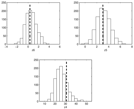
Figure 1: Histograms of the $z_{j}$ statistics for 1000 simulations of beam smoothed, constant power ($\ell(\ell+1)C_{\ell}=$ constant) large-angular-scale maps, $\ell\leq 28$. The dashed lines correspond to the values of $z_{j}$ for the actual DMR 53+90 GHz DMR.

We apply our statistic to test for structure in the COBE DMR map. Figure 1 shows histograms of the $z_{j}$ (Eq. 6) for 1000 simulations of large-angular-scale maps $\ell\leq 28$, with $\ell(\ell+1)C_{\ell}=(24\pi/5)Q^{2}_{\rm rms-PS}$, with $Q_{\rm rms-PS}=15.3\,\mu$K, $7\mbox{${}^{\circ}$}$ FWHM beam smoothing and the noise level of the DMR 53+90 GHz map. The dashed lines in the figure correspond to the actual values of $z_{j}$ for the DMR 53+90 GHz map. The values are consistent with those expected from the simulations. Both the simulations and the DMR maps have a $20\mbox{${}^{\circ}$}$ galactic cut. SHW are easily adaptable to sky maps with Galactic cuts or with any others kinds of gaps. The wavelet functions are still orthogonal and the null distributions are exactly as before (with smaller $k_{j}$). We note that with only a $10\mbox{${}^{\circ}$}$ galactic cut (i.e., with considerable galactic contamination) the values of the $z_{j}$ obtained from the DMR maps are 71.2, 5.9, and 1.6 for $j=4$, 5 and 6, respectively. The histograms representing the simulations, which have only a CMB signal in them, remain virtually unchanged. As expected, more significant structure is detected when some of the galactic signal is present, and this structure is not consistent with a cosmological signal alone.

At resolution 4 the mean of the simulations and the actual map are both considerably displaced from zero. At resolution 5 $z_{5}$ is somewhat less displaced from zero and at resolution 6 $z_{6}$ is consistent with zero. This is consistent with the beam scale being right around the pixel size at resolution 5 so there is structure on that scale and at the lower resolution, but no structure at the higher resolution.

As an aside, note that the covariance matrix ${\mathbf{\Sigma}}_{\gamma}=\langle\vec{\gamma}\vec{\gamma}\rangle$ of $\vec{\gamma}$ is

$${\mathbf{\Sigma}}_{\gamma}={\bf W}({\bf C}+{\mathbf{\Sigma}}_{\rm noise}){\bf W}^{t},$$ (7)

where ${\bf C}$ and ${\mathbf{\Sigma}}_{\rm noise}$ are the covariance matrices of the model and noise, respectively. In general the matrix ${\mathbf{\Delta}}$, which is used to transform the covariance matrix of $\vec{\lambda}$ to the identity, is

$${\mathbf{\Delta}}={\mathbf{\Sigma}}_{\gamma}^{-1/2}.$$ (8)

If we take no correlations from a cosmological model (${\bf C}=0$) and the noise is uncorrelated and homoscedastic (i.e., ${\mathbf{\Sigma}}_{\rm noise}\propto{\bf I}$), then ${\mathbf{\Sigma}}_{\gamma}$ is diagonal. But ${\mathbf{\Sigma}}_{\gamma}$ is a lot more complicated when a cosmological model is assumed.

Our analysis has not taken full advantage of the localization properties of wavelets. SHW can easily yield a spatial decomposition. First, divide the sky into $P$ disjoint patches. Each patch $i$ can be represented as $\vec{\lambda}_{J,i}$ by filling with zeros those pixels not in patch $i$. All the $\vec{\lambda}_{J,i}$ are orthogonal and

$${\rm RMS}^{2}=\frac{1}{w}[(\vec{\lambda}_{J,1})^{t}\vec{\lambda}_{J,1}+\cdots+(\vec{\lambda}_{J,P})^{t}\vec{\lambda}_{J,P}].$$

An angular-scale decomposition like (5) can now be applied to every term.

3 Wavelet Denoising of a Map

In the following sections we apply wavelet denoising with two different applications in mind. In the first application denoising will be used to identify and remove localized sources from a CMB map. In the second application denoising will be used to suppress instrumental, or other non-localized noise, and compress a map. In both operations we use the same denoising technique. The techniques discussed are applicable to both spherical and flat space wavelets. Both types of wavelets will be considered.

Let $d_{i}$ be the measured temperature in pixel $i$, we write $d_{i}=T_{s,i}+F_{i}+n_{i}$, where $T_{s,i}$ is the underlying temperature at pixel $i$, $F_{i}$ is a foreground source temperature, and $n_{i}$ is a noise term describing noise sources which are not localized on the sky (e.g., instrumental, atmospheric ). The assumptions we make about $T_{s,i}$ depend on whether we remove sources or suppress noise in a map. In the first case we assume that $T_{s,i}$ and $n_{i}$ have zero mean and are uncorrelated, and that $F_{i}$ is fixed and unknown. $T_{s,i}$ is assumed random, drawn from some power spectrum, and we attempt to discriminate fixed sources from random realizations of ${{\bf T}}_{s}$ in our sky. In the second application, when suppressing noise in a map, both $T_{s,i}$ and $F_{i}$ are assumed fixed. The goal is to suppress $n_{i}$ and thus obtain a better estimate of the actual realization of the signal in our sky.

In either case the procedure consists of ‘denoising’ by thresholding the wavelet coefficients of the data and transforming back. The difference between the two cases arises in what is assumed as noise during the thresholding stage. This will be discussed in Section 3.2. We start by computing the wavelet transform of the map. Wavelet coefficients are then either set to or shrunk towards zero depending on whether their absolute values are above or below a chosen threshold. Finally we compute the inverse wavelet transform of the thresholded coefficients. We call this procedure ‘denoising’ (see Donoho 1992 for a discussion of this term.) Although the procedure is similar to the one often used with Fourier coefficients, Donoho (1992) showed that wavelet denoising efficiently supresses noise while preserving the sharpness of the original signal. This property makes wavelet denoising appealing for our applications.

3.1 Thresholding

‘Thresholding’ is a prescription for using the sample wavelet coefficients $\gamma_{j,m}$ to estimate the true wavelet coefficients, i.e., the wavelet coefficients of the noiseless map. We use thresholding functions of the form (Donoho 1992)

$$\delta(\gamma_{j,m})=\left\{\begin{array}[]{ll}\gamma_{j,m}-\tau_{j}&\mbox{if $\gamma_{j,m}\geq\tau_{j}$}\\ 0&\mbox{if $|\gamma_{j,m}|<\tau_{j}$}\\ \gamma_{j,m}+\tau_{j}&\mbox{if $\gamma_{j,m}\leq-\tau_{j}$},\end{array}\right.$$ (9)

where $\gamma_{j,m}$ is a wavelet coefficient of the map and $\tau_{j}$ is a chosen threshold at scale $j$. A thresholding scheme corresponds to a particular prescription for choosing the $\tau_{j}$. The $\gamma_{j,m}$ are now replaced by the $\delta(\gamma_{j,m})$ which are used as the “denoised” wavelet coeffecients.

Given a coarsest resolution $J_{o}$, Donoho & Johnstone (1994) suggest keeping the coefficients $\lambda_{J_{o}}$ where the signal dominates the noise and thresholding the rest. Wavelet thresholding is an active area of research. Comparing different thresholding methods is outside the scope of this paper. See Nason (1995) for a survey of thresholding methods. We use the SureShrink procedure of Donoho & Johnstone (1995). Ideally one wants to use the threshold that minimizes the mean square error (MSE)

$${\rm MSE}=\langle\sum_{m}(\delta(\gamma_{j,m})-\mu_{j,m})^{2}\rangle,$$ (10)

where $\mu_{j,m}$ is the mean of the coefficient $\gamma_{j,m}$. However, the means $\mu_{j,m}$ are unknown and therefore so is the MSE (10). To overcome this difficulty SureShrink uses Stein’s unbiased estimate of the MSE (see Donoho 1992). SureShrink selects a threshold $\tau_{j}$ at each scale $j$ that is the best, for rules of the form (9), in the sense that it minimizes Stein’s estimate of the MSE (10). The computational cost at each level is $O(k_{j}{\rm log}(k_{j}))$. Denoising a map with gaps is done in exactly the same way but using only those coefficients based on pixels outside the gaps (see Appendix).

SureShrink wavelet thresholding is asymptotically minimax (Donoho & Johnstone 1995), i.e., it minimizes the worst possible mean square error of the wavelet coefficients estimates. Under certain conditions minimax estimators are posterior Bayesian estimates given a least favorable prior, see Lehmann & Casella (1998) for a more complete discussion regarding the relation between minimax and Bayesian estimators.

3.2 Noise

Denoising requires information about what constitutes noise and what its distribution is. When we use wavelets to identify foreground sources, $F_{i}$, both the cosmological signal $T_{s,i}$ and the noise $n_{i}$ are assumed to be random components of the noise that contaminates the wavelet coefficients, i.e., $\sigma^{2}=\sigma_{\rm CMB}^{2}+\sigma_{\rm noise}^{2}$, and the denoised wavelet coeffecients are identified with the sources alone. In the second application, when we only suppress noise in a map, only $n_{i}$ is considered noise, i.e., $\sigma=\sigma_{\rm noise}$, and the signal component is taken to be the cosmological CMB component, $T_{s,i}$. These values of $\sigma$ are used by SureShrink to compute the estimate of the MSE (10).

In this paper we assume that pixel noise is uncorrelated and Gaussian. This was approximately the case for the DMR maps (Lineweaver et al. 1994) but it may not be a reasonable assumption for other experiments. For cases where the noise is correlated we point out the following. If the correlation structure is known then the map can be transformed to the uncorrelated case; however, depending on the size of the covariance matrix, such a transformation might be computationally expensive. Moreover, this transformation is not appropriate when searching for localized sources because it destroys and widens their shape. More generally, such a decorrelating transformation no longer gives a “sky map”, but a linear combination of sky pixels. Only in the case of suitably mild correlations can such a decorrelated dataset still be considered a map per se. One should also note that for the process of identifying localized sources, when the signal $T_{s,i}$ is considered part of the noise, the cosmological correlation of $T_{s,i}$ must also be included in the noise correlation structure. Depending on the amount of correlation, normalizing only by the variance (as for uncorrelated noise in Section 2) may be sufficient. Johnstone & Silverman (1997) show that SureShrink still works well under mild conditions on the correlation structure. They show that long range correlations in the data are reduced by the wavelet transform, that there is almost no correlation between coefficients from different scales, and that Stein’s MSE estimate is still unbiased.

4 Estimation and Removal of Point Sources with Wavelets

We now use the denoising procedure to reduce localized source contamination in sky maps. Here $T_{s,i}$ and $n_{i}$ are assumed to have zero mean and to be uncorrelated, while $F_{i}$ is fixed and unknown. The goal is to estimate the foreground source field ${{\bf F}}$. Since the noise and the cosmological model have zero mean (we assume that the CMB monopole has been subtracted), uncontaminated denoised wavelet coefficients should be close to zero. Our goal is to find an estimate $\hat{{\bf F}}$ of the foreground field ${{\bf F}}$ by thresholding the wavelet coefficients. We then use a criterion to identify sources in the field. We suggest masking pixels in identified locations.

To estimate the source field we normalize the coefficients using the matrix ${\mathbf{\Delta}}$ defined by Equation (8). To estimate the variability of the wavelet coefficients at each resolution, i.e., the diagonal elements of ${\mathbf{\Delta}}$, we use the median absolute deviation. This measure is resistant to outliers and thus less affected by point sources. Once coefficients have been normalized they are denoised using SureShrink. By assumption, the means in Eq. 10 satisfy $\mu_{j,m}=0$ for all $\gamma_{j,m}$ not contaminated by sources.

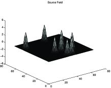
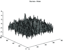
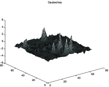
Figure 2: Estimating a source field (top left) from a noisy source field (top right) by thresholding Haar (bottom left) or Daubechies (bottom right) wavelet coefficients. All sources have identical signal, and the s/n is 3, where s/n is defined as (peak amplitude)/(RMS noise). Daubechies wavelets yield higher s/n estimates of the source location and shape.

Using SHW on the whole sky has some drawbacks. First, SHW are not smooth and therefore do not provide good estimates of smooth peaks of localized sources. (Localized sources are at least as broad and smooth as the beam of the experiment.) Also, since local sources are sparse they are difficult to detect when considering the entire sky. For noise dominated data SureShrink uses a large threshold proportional to $\sqrt{{\rm log}(k_{j})}$. These two problems are alleviated by taking smaller sky sections where smooth planar wavelets can be used. Patches are easily defined through the map pixelization by taking lower resolution pixels as patches. On each patch we use tensor products of one-dimensional Daubechies wavelets. (We found that better results were obtained with four vanishing moments, and that other wavelet bases do not lead to significantly different results from those obtained with Daubechies wavelets.) Note that SHW on small patches reduce to tensor products of Haar wavelets. Figure 2 shows the original (six sources of the same amplitude) and original plus white noise (s/n = 3, where s/n is the ratio of the peak amplitude to the noise RMS) source fields on a patch, and thresholded estimates using planar Haar and Daubechies wavelets. Daubechies wavelets recover the peaks of the sources better than Haar wavelets. Hence we use Daubechies wavelets for point source identification and removal. Note also that source estimates are very close to flat wherever there are no sources. This minimizes potential systematic effects arising from false source identification.

4.1 Single Source in White Noise

To learn about the denoising process we first apply the procedure to a single source buried in white noise. Table 2 (left) shows the relative error in reconstructing the source. We calculate RMS$({{\bf F}}-\hat{{\bf F}})/{\rm RMS}({{\bf F}})$ inside the source, where ‘inside’ is defined as pixels where ${{\bf F}}>1\%$ of the noise RMS. This measure of relative error is an indication of power in the source field not accounted for in the estimated field. The s/n is the ratio of the source peak to the noise RMS. The size is the ratio between the number of pixels inside the source and the total number of pixels in the patch in percent. The first and second rows correspond to Haar and Daubechies wavelets, respectively. In all cases Daubechies wavelets yield smaller relative errors. In Table 2 (right) we quantify to what extent the wavelet thresholding affects regions originally not contaminated by the source. We calculate the ratio RMS$({{\bf F}}-\hat{{\bf F}})/{\rm RMS}({\rm noise})$ outside the source. The table shows that the ripples introduced in the originally uncontaminated region have an amplitude of less than 20% of the noise RMS, well within the noise level, and that this amplitude is very nearly constant with source size.

4.2 Spectrum of Source Intensity

We will now attempt to identify and remove a more realistic distribution of sources from a map. We generate a source field using a power-law

$$dN(s)\propto s^{-2.5}ds,$$ (11)

where $N$ is the number of sources and $s$ is signal-to-noise ratio. (As before, s/n is the ratio of peak amplitude and noise RMS.) Source centers are randomly distributed on the patch and only sources with $s>1$ are included. The power-law exponent, $-2.5$, is appropriate for a population of sources with a single luminosity distributed randomly through an infinite, flat, euclidean space. The total number of sources in the patch is determined by the choice of different ratios (total area inside sources)/(total patch area), where ‘inside’ is defined as in the previous section. The noise is assumed to be either white or characterized by a Gaussian correlation function with damping scale as a fraction of the maximum wavenumber. We used two Gaussian random fields, $G_{1}$ and $G_{2}$, with damping scales 0.8 and 0.6, respectively. The field $G_{1}$ has correlations of approximately 12%, 2% and 1% between first, second and third neighbors, respectively. The correlations for the second Gaussian field, $G_{2}$, are 20%, 3% and 1%. Rather than using a particular CMB model, we used the Gaussian correlated noise as a generic model for a correlated signal. As we will see our results are not sensitive to the particular correlation structure assumed.

To determine source locations in the thresholded map we perform a second thresholding on $\hat{{\bf F}}$. This is done by comparing pixel absolute magnitudes with $k\times({\rm MAD})$, where MAD is the median absolute deviation of $\hat{{\bf F}}$, for different values of the threshold $k$.

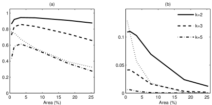
Figure 3: (a) Proportion of correctly detected source pixels that were above 1$\sigma$ as a function of Area for different thresholds $k\times$MAD. ‘Area’ is the fraction of pixels covered with sources, $k$ is an integer and MAD is the mean absolute deviation of the denoised map - see text for more details. (b) Proportion of pixels outside the source that were incorrectly identified as source pixels. As a comparison, the dotted lines correspond to the process of detecting source pixels by setting a simple $1\,\sigma$ cut on the map.

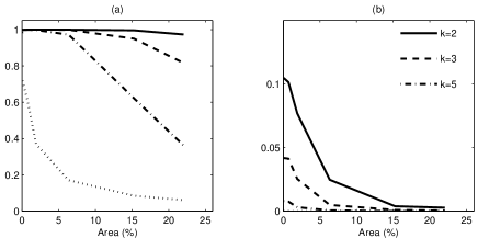
Figure 4: (a) Proportion of correctly detected source pixels that were above 3$\sigma$ as a function of Area for different thresholds $k\times$MAD. ‘Area’ is the fraction of pixels covered with sources, $k$ is an integer and MAD is the mean absolute deviation of the denoised map - see text for more details. (b) Proportion of pixels outside the source that were incorrectly identified as source pixels. As a comparison, the dotted lines correspond to the process of detecting source pixels by setting a simple $3\,\sigma$ cut on the map.

Figures 3, 4 show the results of the point-source identification process for sources that were above $1\sigma$ and $3\sigma$, respectively. For each figure, plate (a) shows the proportion of correctly identified source pixels for $k=2,3,5$ and plate (b) shows the proportion of pixels outside sources that were incorrectly identified as source pixels, for the same $k$ values. The area is defined as the proportion of source pixels above $1\sigma$. As $k$ increases the probability of correct detection decreases as does that of incorrect detections. The results in Figures 3, 4 are for sources in white noise but no significant difference was observed with Gaussian correlated noise. Even a Gaussian field with damping scale 0.3 did not show significant differences.

The figures show that wavelets are extremely effective in identifying point sources. When we are looking for sources of moderate s/n (Figure 4) which cover up to $\simeq 5\%$ of the patch area, virtually all source pixels are identified regardless of the value of $k$. For low s/n sources (Figure 3), a criterion of $k<3$ identifies more than 80% of the source pixels. Comparing Figures 3 and 4 we see that for wavelet thresholding the proportion of false detections does not change much with the s/n of the source being searched for. In addition, simulations show that when there are no sources in the patch only about 1% of the pixels in the patch are incorrectly identified as sources. To reduce the number of ‘incorrect detections’ over the entire map, which presumably consists of many patches, we may choose not to subject every patch to this source cleaning procedure. Rather, it may be advantageous to first calculate the value of $z_{j}$ for the patch, as described in Section 2, and then proceed with the source cleaning procedure only on patches with abnormally large values of $z_{j}$ at some scale $j$. Further analysis and simulations are necessary to optimize the method.

One can compare the performance of wavelets in identifying point sources to the performance achieved by a number of alternative techniques. A detailed study is in progress. Here we only compare with the simple practice of removing map pixels whose amplitudes are larger than $k\sigma$, where $\sigma$ is the RMS of the noisy source field. The dotted lines in Figures 3, 4 correspond to a $1\sigma$ and $3\sigma$ cuts, respectively. Wavelets achieve a significantly higher proportion of correct detections, and less errors are made when searching for low s/n sources. Interestingly, the $k\sigma$ cut has fewer errors when searching for high s/n sources. That suggests that the optimal point source identification procedure may involve a combination of techniques, with wavelets being the leading tool.

Table 2: Left: Relative error RMS$({{\bf F}}-\hat{{\bf F}})/{\rm RMS}({{\bf F}})$ in estimating a field with a single source embedded in white noise. The relative error is calculated using only pixels inside the source, where ’inside’ is defined in the text. The s/n is the ratio of the source peak to the noise RMS. The size is the percentage of pixels of the patch inside the source. The first and second rows correspond to Haar and Daubechies wavelets respectively. Right: the ratio of the residual RMS to the noise RMS outside the source.

size (%) s/n 18 11 5 3 1 2 .33 .64 .83 1.02 1.34 .26 .53 .73 .93 1.28 4 .23 .41 .52 .63 .81 .17 .29 .40 .51 .74 6 .19 .32 .42 .52 .67 .13 .22 .31 .41 .57

size (%) 18 11 5 3 1 .11 .11 .11 .11 .10 .12 .11 .11 .11 .10 .15 .15 .15 .15 .15 .16 .16 .16 .16 .15 .17 .16 .16 .16 .16 .17 .16 .16 .16 .16

5 Map Denoising and Compression

In this section we apply wavelet denoising with the goal of compressing information and reducing noise for visualisation of CMB maps. Denoised maps are useful for displaying or transmitting compressed map files.

Here we assume that the CMB sky, ${{\bf T}}_{s}$, is fixed and that the random field we are trying to isolate and remove is the instrumental noise. Hence, only the noise variability is included in the matrix ${\mathbf{\Delta}}$ (Eq. 8), and it is estimated using only the wavelet coefficients at the highest resolution where we expect little structure. Alternatively, ${\mathbf{\Delta}}$ could be estimated using the difference of two independent maps (as with the $A-B$ DMR maps). This time SureShrink determines the threshold $\tau_{j}$ that minimizes (10) with $\mu_{j,m}$ being the unknown wavelet coefficients of the fixed sky ${{\bf T}}_{s}$. The denoised estimate of ${{\bf T}}_{s}$ is then ${\bf W}^{-1}\delta(\gamma)$, the inverse transform of the thresholded coefficients. The computational cost is $O(N{\rm log}(N))$. Note also that the estimate of the underlying temperature field achieved in this process is model independent. In other words, it did not require a cosmological model.

In other work Wiener filtering has been used for denoising CMB maps (Bunn et al. 1996). The Wiener filter estimate of ${{\bf T}}_{s}$ is ${\bf C}{{\bf d}}$, where the matrix ${\bf C}$ is determined by assuming a cosmological model for ${{\bf T}}_{s}$ and minimizing $\langle||{\bf C}{{\bf d}}-{{\bf T}}_{s}||^{2}\rangle$. The process takes $O(N^{3})$ operations and depends on the fiducial model chosen. Thus, while Wiener filtering provides a posterior mean estimate given a prior cosmological model, wavelet thresholding provides an estimate of the actual realization of the unknown field without assuming a cosmological model. The Wiener filter can be defined as the maximum-probability signal contribution given the data, the underlying signal power spectrum and noise correlation, and assuming Gaussianity for both signal and noise. SureShrink wavelet thresholding, on the other hand, is aymptotically minimax (see Section 3.1 and Donoho & Johnstone 1995).

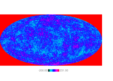
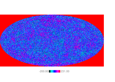
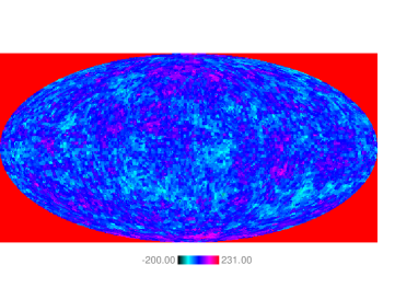
Figure 5: Top: a simulated, signal only, CMB map based on a standard CDM model. There are about 98000 pixels in the map. Middle: the signal map with noise added. The s/n in this map is $\approx.7$. Bottom: The noisy map after denoising with SureShrink. Only 14% of the wavelet coefficients were used, and the denoising process took less than 6 seconds on an Alpha 500/266 workstation.

Figure 5 shows the denoising of a simulated standard CDM map with $\Omega_{b}=.05$, $\Omega=1$, $H_{0}=50$ km/s/Mpc. The signal to noise in the signal plus noise map (middle) is $\approx.7$, where the signal to noise is the ratio of the noise RMS to the signal RMS. There are 98304 pixels in the map. The denoised map (bottom) achieved a 35% noise reduction, as measured by the ratio RMS(true map - denoised map)/(noise RMS), using only $14\%$ of the 98304 wavelet coefficients. It also has only 14% of the original number of pixels, but pixels have a variety of sizes, adapted to the local structure as identified by the thresholding procedure. The entire denoising process took less than 6 seconds on an Alpha 500/266 workstation. The compression rate that denoising can achieve depends on the signal to noise. As it increases more coefficients have to be used. Table 3 shows the noise reduction and compression rate for different signal to noise ratios using the same standard CDM model.

Wavelet denoising is a flexible procedure in that it allows one to choose the threshold level which will achieve a particular compression rate regardless of the denoising achieved. In our case the thresholds were chosen to minimize an estimate of the mean square error (10) but this may not be the optimal procedure. Depending on the goal at hand one may be able to devise a thresholding procedure tailored for a particular task.

Table 3: Noise reduction and compression achieved by SureShrink denoising of a standard CDM model for different signal to noise ratios.

signal/noise	RMS(residuals)/RMS(noise)	% coefficients used
.9	.82	33
.7	.65	14
.6	.57	7

6 SHW and Cosmological Information

It has become traditional to consider the cosmological information from CMB datasets in the context of likelihood functions, usually expressed in pixels or in the spherical harmonic domain. Since no information is lost by transforming to wavelet space we can ask whether it is better to work in wavelet domain when the goal is to estimate $C_{\ell}$s and cosmological parameters.

Assuming Gaussianity of both the cosmological signal and the noise, the log-likelihood of the data given a model with covariance matrix ${\bf M}$ is

$$-2{\rm ln}\,{\cal L}(p_{i}|{\bf d}) = {\rm ln}\,|{\bf M}|+{\bf d}^{t}{\bf M}^{-1}{\bf d}$$ (12)

$$= {\rm ln}\,|{\mathbf{\Sigma}}_{\gamma}|+\gamma^{t}{\bf W}^{-t}{\bf M}^{-1}{\bf W}^{-1}\gamma$$

(up to an additive constant) where $p_{i}$ are the cosmological parameters and $\gamma={\bf W}{\bf d}$ is the wavelet transform of the data ${\bf d}$. ${\bf M}={\bf C}+{\mathbf{\Sigma}}_{\rm noise}$ is the sum of contributions from the signal and the noise covariance. In the second equality we have transformed from the map pixel basis to the wavelet domain (see also Eq. 7). To estimate the $p_{i}$ it is enough to consider the eigenmodes of ${\bf C}$ which contribute the most to ${\cal L}$ (this is the Karhunen-Loeve or “signal-to-noise eigenmode” transformation, Bond 1995). This simplifies the likelihood by compressing the data. The reduced likelihood can be used to estimate cosmological parameters.

Can we apply the same technique on the thresholded wavelet coefficients? Because the thresholding procedure is nonlinear the distribution of the denoised $\gamma=\delta(\gamma)$ is no longer Gaussian and therefore Eq. 12 written in terms of $\delta$ is no longer the correct log-likelihood. It is computationally expensive to compute the correct likelihood function of the thresholded coefficients for each plausible cosmological model. We can still maximize Eq. 12, with respect to $p_{i}$, to estimate the parameters but the perfomance of this procedure is still to be investigated.

The difficulties due to the non-linearity of the wavelet thresholding process can perhaps be resolved by treating the process as a linear operation. That is, we consider the thresholding operation of Eq. 9 as if the thresholds $\tau_{j}$ are fixed beforehand. Then, the new wavelets coeffecients $\delta(\gamma_{j,m})$ can be considered as linearly related to the old coeffecients: $\delta(\gamma_{j,m})=\alpha_{jm}\gamma_{j,m}$. This is similar to, for example, Wiener filtering, where each Fourier mode is modified by some factor $0\leq\alpha_{k}\leq 1$ (although in that case the process is strictly linear since the $\alpha_{k}$ do not depend upon the data). Thus, the denoised wavelet coeffecients can be considered a much smaller linear rendition of the original data. The correlation structure may indeed be much more complicated than the raw data, but because there may be many fewer coefficients, the $O(N^{3})$ operations necessary for manipulating the likelihood are much faster. This procedure is under further investigation.

Since working with the denoised coefficients seems problematic one could use the likelihood without denoising the coefficients. But then nothing seems to be gained by working in wavelet domain since the quadratic term in (12) does not split into independent components of different scales—the second equality above is not easier to compute than its version in the pixel domain. Consider, for example, a quadratic estimator $\lambda_{J}^{t}{\bf E}\lambda_{J}$ of $C_{\ell}$ (e.g., Tegmark 1997; Bond, Jaffe & Knox 1998). Since the wavelet transform acts as a band-pass filter, one might hope to reduce leakage and decrease computational cost by considering only high resolution coefficients to estimate small-angular-scale (large $\ell$) $C_{\ell}$, splitting $\lambda_{J}^{t}{\bf E}\lambda_{J}$ as in (5) and taking only high resolution coefficients. There are three problems: (1) Spherical harmonics have components in the lower wavelet scales (Table 1) that need to be estimated; (2) Wavelet coefficients $\lambda_{j}$ are orthonormal with respect to the identity but not with respect to any matrix ${\bf E}$. In general the cross terms in a quadratic estimator using a decomposition of the form (5) do not cancel; (3) The number of coefficients at each scale grows exponentially; using only the highest resolutions yields little compression. For example, 93% of the coefficients of a resolution 10 map belong to the two highest resolutions. Because of these problems, the estimator (like the likelihood function itself above) does not appear to be any easier to compute in the wavelet domain.

Figure 6: Histograms of the $z_{4}$ statistic for the same kind of simulations as in Figure 1 but with spectral index $n=0.5$ (instead of $n=1$), where $n$ is the spectral index of the primordial desnity fluctuation power spectrum which in turn gives $\ell(\ell+1)C_{\ell}\propto\ell^{n-1}$. The distribution of $z_{4}$ under this model is clearly different from that of the $n=1$ model (Figure 1). The dashed line indicates the value of $z_{4}$ for the DMR 53+90 GHz map.

Another approach is to consider using the wavelet coefficients themselves as intermediate parameters in the process of cosmological parameter estimation. A homogeneous random field is characterized by its power spectrum $C_{\ell}$, which is in turn parametrized by the cosmological parameters. In principle cosmological parameters can be estimated by fitting to the $C_{\ell}$. Power in the wavelet domain provides some information about cosmological parameters. For example, Figure 6 shows the distribution of the normalized power at resolution 4 ($z_{4}$) for the same large-angular-scale models of Figure 1 but now using $n=0.5$ (instead of $n=1$), where $n$ is the spectral index of the primordial density fluctuation power spectrum which in turn gives $\ell(\ell+1)C_{\ell}\propto\ell^{n-1}$. Comparing this histogram to the one in Figure 1 it is obvious that the distribution of $z_{4}$ can discriminate between the two models. However, even future high resolution CMB maps will only be of resolutions $j\leq 10$, and only the highest resolutions $j\geq 7$ will be most useful for extracting cosmological parameters . Using the wavelet power at scales $j=7,8,9,10$ will not yield enough degrees of freedom to fit 11 cosmological parameters. This paucity of information in the wavelet domain is because the number of independent wavelet power coefficients (the $z_{j}$s) scales only as the logarithm of the number of pixels. In contrast the number of independent power spectrum coeffecients $C_{\ell}$ (which completely determine the properties of the homogeneous and isotropic Gaussian CMB field) scales as the square root of the number of pixels. Using the wavelet power as we have defined it here will not be sufficient.

We could instead consider abandoning both $C_{\ell}$ and the wavelet power defined here in exchange for a spectrum more localized in both location and scale. The question is whether we can find a spectral representation of homogeneous random fields on the sphere in terms of localized functions. However, it is easy to show that there is no smooth basis $\{\Psi_{i,j}\}$, with local support decreasing with $j$, with the property that any homogeneous random field on the sphere can be written as $\sum_{i,j}\alpha_{i,j}\Psi_{i,j}$ where $\langle\alpha_{i,j},\alpha_{i^{\prime},j^{\prime}}\rangle=\sigma_{j}^{2}\delta_{i}^{i^{\prime}}\delta_{j}^{j^{\prime}}$. That is, any other “power spectrum” we define in terms of locally supported functions will have an extended “window function” in $\ell$, as with the wavelet coeffecients of Section 2; the usual $C_{\ell}$ spectrum is still the most natural choice.

7 Summary

Wavelets provide a useful tool to investigate local structure in maps. We used SHW to define a local measure of power that is equivalent to a normalized local angular scale decomposition of the map RMS. This measure can be used to compare power in different regions in the sky. Similar measures can be defined with other bases of orthogonal wavelets. SHW have the advantage of being easily implemented given any map pixelization scheme. SHW can also be used to denoise and compress maps without doing any diagonalization or inversion of matrices. We denoised and compressed a 100,000 pixel CMB map by a factor of $\sim 10$ in 5 seconds achieving a noise reduction of about 35%. In contrast to Wiener filtering the compression process is model independent. The total computational cost of wavelet transforming and thresholding a region with $N$ pixels is $O(N{\rm log}(N))$.

Since wavelets are locally supported they can be used to reduce localized source contamination in maps. We applied planar Daubechies wavelets for the identification and removal of points sources from small planar-like sections of sky maps. Our technique successfully identified most point sources which are above $3\sigma$ and more than 80% of those above $1\sigma$. In addition, wavelet thresholded estimates of source fields introduce little structure in uncontaminated regions.

We have concentrated on local source detection and map compression. We did not find useful direct applications of spherical wavelets to the estimation of angular power spectra or cosmological parameters. Ideally we would like to have a wavelet basis which approximately diagonalizes the covariance matrix of the comological model as well as the noise covariance matrix, thus simplifying the likelihood function. This is not the case for SHW. But in the future there may be hope for spherical wavelets that are more compatible with spherical harmonics. See for example Freeden & Windheuser (1997), and references therein. They define smooth spherical wavelets that combine a spherical harmonic expansion for the low order terms and wavelet expansions for the small scale structure. However, they do not yet have a fast wavelet transform.

In Section 3.1 we pointed out that SureShrink wavelet thresholding provides posterior estimates for a priori distributions of the wavelet coefficients that give the largest mean square error. Although we have not used them there are also Bayesian thresholding methods that can be used to include more informative prior information on the wavelet coefficients. See Abramovich et al. (1997) and references therein. The development of wavelet tools in statistics is a very active field of research. For a review see Silverman (1999) as well as the other articles in the same volume.

The computer code used for work presented in this paper will soon be freely available at
http://cfpa.berkeley.edu/combat.

Acknowledgements. This work was done under the auspices of the COMBAT collaboration supported by the NASA AISR program, grant NAG5-3941. We are grateful to L. Cayón, D. Donoho , P. Ferreira and P. Stark for helpful suggestions. Simulations of CMB maps were simplified thanks to Seljack & Zaldarriaga’s CMBfast and E.Scannapieco’s CMAP (http://cfpa.berkeley.edu/combat). We thank G. Smoot for allowing access to his Alpha cluster. S.H. was partially supported by NASA grant NAG5-3941, A.J. by NASA LTSA NAG5-6552, and L.T. by grants NAG5-3941 and DMS-9404276. Part of this work uses the Wavelab package, available from http://www-stat.stanford.edu/wavelab/.

Appendix A Haar Wavelets for the COBE Pixelization

Spherical Haar wavelets (Sweldens 1995, Schroeder & Sweldens 1995) are a generalization of planar Haar wavelets. To define SHW we need a hierarchical pixelization scheme. One example of such is the COBE sky cube (CSC) pixelization where the surface of the unit sphere is divided into $6\cdot 4^{(j-1)}$ approximately equal area pixels at resolution $j$. Each pixel $k$ at resolution $j$, $S_{j,k}$, has four children, $S_{j+1,k_{1}},...,S_{j+1,k_{4}}$, at resolution $j+1$. Let ${\it K}(j)$ be the pixel numbers corresponding to resolution $j$.

The functions that model the main features of the data at each scale are scaling functions, and the functions that represent the details of the data not captured by the scaling functions are the wavelets. The scaling functions of the SHW are defined as $\varphi_{j,k}(\eta)=1,$ if $\eta\in S_{j,k}$ and 0 otherwise. Define $V_{j}\subset L_{2}$ as the closed subspace generated by the $\varphi_{j,k}$: $V_{j}={\rm clos}\{\varphi_{j,k}|\,\,k\in{\it K}(j)\}.$ For example, a DMR sky map is an element of $V_{6}$. By definition $V_{j}\subset V_{j+1}$. The SHW are defined as an orthogonal basis for the orthogonal complement, $W_{j}$, of $V_{j}$ in $V_{j+1}$. By construction, for any chosen $J$, $V_{J}=V_{j}\bigoplus_{i=j}^{J-1}W_{i}.$ For example, a resolution 10 map is a sum of a coarser resolution 9 map plus a function from $W_{9}$ encoding the details not captured by the coarser map, or a resolution 8 map plus detail functions from $W_{8}$ and $W_{9}$. The functions that capture the leftover details are combinations of the wavelets at different resolutions: there are three wavelets, $\psi_{j,m_{1}}\psi_{j,m_{2}},\psi_{j,m_{3}}$, associated to each pixel $S_{j,k}$. Let $\mu_{j,k}$ be the area of pixel $S_{j,k}$ and ${\it L}(j,k)=\{m_{o}(k),m_{1}(k),m_{2}(k),m_{3}(k)\}$ be the pixel numbers of its four children, then the three wavelets for pixel $S_{j,k}$ are

$$\psi_{j,m_{1}}=\frac{\varphi_{j+1,m_{o}}+\varphi_{j+1,m_{3}}}{2\mu_{j+1,m_{o}}+2\mu_{j+1,m_{3}}}-\frac{\varphi_{j+1,m_{1}}+\varphi_{j+1,m_{2}}}{2\mu_{j+1,m_{1}}+2\mu_{j+1,m_{2}}}$$

$$\psi_{j,m_{2}}=\frac{\varphi_{j+1,m_{1}}}{2\mu_{j+1,m_{1}}}-\frac{\varphi_{j+1,m_{2}}}{2\mu_{j+1,m_{2}}}$$

$$\psi_{j,m_{3}}=\frac{\varphi_{j+1,m_{o}}}{2\mu_{j+1,m_{o}}}-\frac{\varphi_{j+1,m_{3}}}{2\mu_{j+1,m_{3}}}$$

The wavelets $\{\psi_{j,m_{i}(k)}|\,\,i=1,2,3;\,\,k\in{\it K}(j)\}$ form a basis for $W_{j}$. In the limit, for any choice of $J_{o}$, $\{\psi_{j,m},j\geq j_{0}\}\cup\{\phi_{j_{0},k}|\,k\in{\it K}(j_{0})\}$ is an orthogonal basis for the space of integrable functions on the sphere. For example, take a function ${\bf T}$ (e.g., a sky map) at a finest resolution level $J$ (i.e., ${{\bf T}}\in V_{J}$) and choose a starting resolution $J_{o}$, then ${{\bf T}}$ can be written as

$$T(i)=\sum_{k\in{\it K}(j_{0})}{\lambda}_{j_{0},k}\varphi_{j_{0},k}(i)+\sum_{j=j_{0}}^{J-1}\sum_{m}\gamma_{j,m}\psi_{j,m}(i).$$ (13)

The first sum corresponds to the lowest resolution map and the second one to the details from the higher resolutions. The coefficients in the expansion (13) define the wavelet transform ${\bf W}{{\bf T}}$ of ${{\bf T}}$

$${\bf W}{{\bf T}} = \vec{\gamma}(\vec{\lambda}_{j_{o}},\vec{\gamma}_{jo},\cdots,\vec{\gamma}_{J-1})^{t}$$ (14)

$$= (\{\vec{\lambda}_{J_{o},k},k\in{\it K}(J_{o})\},\{\vec{\gamma}_{j,m},$$

$$m\in{\it M}(j),J_{o}\leq j\leq J-1\})^{t}.$$

No linear system needs to be solved in order to compute the components of $\vec{\gamma}$, they are obtained recursively starting from the finest resolution coefficients $\vec{\lambda}_{J}={{\bf T}}$

$$\lambda_{j,k}=\sum_{l\in{\it K}(j+1)}\tilde{h}_{j,k,l}\lambda_{j+1,l},\,\,\,\mbox{and }\gamma_{j,m}=\sum_{l\in{\it K}(j+1)}\tilde{g}_{j,m,l}\lambda_{j+1,l}.$$

To reconstruct a function given the wavelet coefficients we have a recursive inverse transform

$$\lambda_{j+1,l}=\sum_{k\in{\it K}(j)}h_{j,k,l}\lambda_{j,k}+\sum_{m\in{\it M}(j)}g_{j,m,l}\gamma_{j,m}.$$

The coefficients for the forward and inverse transforms defined above are

$$\tilde{h}_{j,k,l}=\left\{\begin{array}[]{ll}\frac{\mu_{j+1,l}}{\mu_{j,k}}&\mbox{if $l\in{\it L}(j,k)$}\\ 0&\mbox{otherwise}\end{array}\right.$$

$$h_{j,k,l}=\left\{\begin{array}[]{ll}1&\mbox{if $l\in{\it L}(j,k)$}\\ 0&\mbox{otherwise}\end{array}\right.$$

$$\tilde{g}_{j,m,l}=\left\{\begin{array}[]{ll}\int_{S_{j+1,l}}\tilde{\psi}_{j,m}\,\,d\mu&\mbox{if $l\in{\it L}(j,k)$}\\ 0&\mbox{otherwise}\end{array}\right.$$

$$g_{j,m,l}=\left\{\begin{array}[]{ll}\frac{1}{\mu_{j+1,k}}\int_{S_{j+1,l}}\psi_{j,m}\,\,d\mu&\mbox{if $l\in{\it L}(j,k)$}\\ 0&\mbox{otherwise,}\end{array}\right.$$

where $\tilde{\psi}_{j,m}$ is the dual of ${\psi}_{j,m}$.

In order to avoid biasing analyses of CMB skies, data contaminated by Galactic emissions or other identified foreground sources are usually discarded. To compute a wavelet transform of data with gaps, we discard those pixels at the lowest resolution $J_{o}$ which are inside the gaps. Only the wavelet coefficients correponding to descendants of pixels outside the gaps are used. Note that the scaling and wavelet functions corresponding to these selected pixels form an orthogonal basis for the sky with gaps. This is due to the local support of the functions and to the vanishing of the integral of $\psi_{j,m}$ over any pixel $S_{j,k}$.

References

- [Abramovich 1997] Abramovich F., Sapatinas T. & Silverman B.W., 1998, J. Roy. Statist. Soc. Ser. B, 60, 725-749
- [Bond 1995] Bond J.R., 1995, Phys. Rev. Lett., 74
- [Bond, Jaffe & Knox 1998] Bond J.R., Jaffe A.H. & Knox L.E., 1998, Phys. Rev. D, in press; astro-ph/9708203
- [Bond et al. 1999] Bond J.R., Crittenden R.C, Jaffe A.H. & Knox L.E., 1999, Computers in Science & Engineering (to appear)
- [Borrill 1999] Borrill J., 1999, Phys. Rev. D, 59, 7302, astro-ph/9712121. See also http://cfpa.berkeley.edu/borrill/cmb/quadest.html
- [Bunn & Sugiyama 1995] Bunn E. & Sugiyama N., 1995, ApJ, 446
- [Bunn et al. 1996] Bunn E., Sugiyama N. & Silk J., 1996, ApJ, 464, 1
- [Cayon 1999] Cayón L. et al., 1999, submitted
- [Donoho 1992] Donoho D.L., 1992, Technical Report, Stanford University
- [Donoho & Johnstone 1994] Donoho D.L. & Johnstone I.M., 1994, Biometrika, 81
- [Donoho & Johnstone 1995] Donoho D.L. & Johnstone I.M., 1995, J. Amer. Statist. Assoc., 90
- [Ferreira et al.] Ferreira P., Magueijo J. & Silk J., 1997, Phys. Rev. D, 56, 4592
- [Freeden & Windheuser 1997] Freeden W. & Windheuser U., 1997, Appl. Comput. Harmonic Anal., 4
- [Hobson, Jones & Lasenby 1999] Hobson M.P., Jones A.W. & Lasenby A.N., 1999, MNRAS, submitted, astro-ph/9810200
- [Johnstone & Silverman 1997] Johnstone I.M. & Silverman B.W., 1997, J. Roy. Statist. Soc. Ser. B, 59, 319-351
- [lehmann] Lehmann E.L. & Casella G., 1998, Theory of Point Estimation, second edition. Springer-Verlag
- [Lineweaver, C.H. et al. 1994] Lineweaver C.H. et al., 1994, ApJ, 436, 2
- [Nason 1995] Nason G.P., 1995, in Wavelets and Statistics, Springer-Verlag, 329
- [Pando, Valls-Gabaud & Fang 1998] Pando J., Valls-Gabaud D. & Fang L., 1998, Phys. Rev. Lett. 81, 4568
- [Sanz et al. 1999] Sanz J.L. et al. , 1999, in Oliveira-Costa A. & Tegmark M., eds, Microwave Foregrounds. ASP, San Francisco
- [Schroeder & Sweldens 1995] Schroeder P. & Sweldens W., 1995, Technical Report, University of South Carolina
- [Silverman 1999] Silverman B.W., 1999, Phil. Trans. R. Soc. Lond. A (to appear)
- [ Sweldens 1995] Sweldens W., 1995, Technical Report, University of South Carolina
- [1] Tegmark M., astro-ph/9611174, Phys. Rev. D, 55, 5895 (1997)