Big Bang Nucleosynthesis: Reprise

Abstract

• Department of Physics, 1 Keble Road, Oxford OX1 3NP, UK

• Abstract. Recent observational and theoretical developments concerning the primordial synthesis of the light elements are reviewed, and the implications for dark matter mentioned.

• Department of Physics, 1 Keble Road, Oxford OX1 3NP, UK

• Abstract. Recent observational and theoretical developments concerning the primordial synthesis of the light elements are reviewed, and the implications for dark matter mentioned.

  1 Introduction

  Why yet another review of big bang nucleosynthesis (BBN)? Given that the basic physics of the synthesis of the light elements D, ³He, ⁴He and ⁷Li in the big bang was thoroughly discussed over 25 years ago [1, 2] it is natural to wonder why so many papers on the subject continue to appear on a regular basis. The reason for this is two-fold. First, as observational determinations of light element abundances have advanced, the situation has become more instead of less uncertain. In particular it has become apparent that inferring the primordial values of the abundances from contemporary observations is fraught with uncertainty, given our limited understanding of the chemical evolution of galaxies. Fortunately observers have risen to the challenge and developed sophisticated techniques to look further back into our past, at nearly pristine primordial material. However large discrepancies, most likely of a systematic nature, have subsequently emerged between different determinations, so the improvement in precision has not led to an increase in accuracy! Nevertheless this is a healthy development in that it has provided a refreshing perspective on the strong claims made in the past decade concerning the consistency of BBN predictions with the inferred primordial abundances, and on the stringent constraints thus inferred on new physics. The second development concerns recent efforts to improve the accuracy of the theoretical predictions of the abundances, and, just as important, to quantify the uncertainties. In this talk I will discuss these issues and summarize their implications for the dark matter problem and for new physics, viz. $N_{\nu}\neq 3$. Other recent reviews [3, 4, 5] may be consulted for a different perspective than mine [6, 7].

  2 Theoretical Calculations

  We now have excellent semi-analytic insights into the physics of BBN which enable the ⁴He abundance to be calculated correctly to within $\sim 1-2\%$ [8] and the ‘left-over’ abundances of D, ³He, and ⁷Li to be estimated to within a factor of $\sim 2-3$ [9]. However for precision work, and in particular, to determine the uncertainties, it is necessary to use the Wagoner computer code [2] which has been improved and updated with the latest values of the nuclear cross-sections and made freely available to the community [10, 11].

  There have been two important developments on this front. First the rates for the weak interactions which determine the neutron-to-proton ratio have been carefully calculated beyond the Born approximation, with allowance for all zero and finite temperature radiative, Coulomb and finite (nucleon) mass corrections [12, 13]. With further allowance for finite temperature QED corrections to the equation of state of the plasma and the residual coupling of the neutrinos to the plasma during $e^{+}e^{-}$ annihilation, the ⁴He abundance has been computed with an accuracy of $\sim 0.4\%$ [12], where the dominant source of uncertainty comes from the present experimental determination of the neutron lifetime: $\tau_{n}=885.3\pm 2.0$ s [14]. This is an impressive feat and it is believed that all relevant physical processes have now been consistently taken into account.

  The uncertainties in the abundances of the other light elements are of course considerably greater and are, moreover, correlated with each other. The standard practice has been to use the Monte Carlo method to sample the error distributions of the relevant reaction cross-sections which are then input into the numerical code, thus enabling well-defined confidence levels to be attached to the theoretically predicted abundances [15, 16]. However this is computationally expensive and, moreover, needs to be repeated each time any of the input parameters are changed or updated. To overcome this handicap we have developed a method based on linear error propagation which requires the numerical code to be run just once to determine the covariance (or error) matrix; simple $\chi^{2}$ statistics can then be used (rather than maximum likelihood methods as with Monte Carlo simulations) to determine e.g. the best-fit value of $\eta\equiv\,n_{\rm N}/n_{\gamma}$, the nucleon-to-photon ratio [17]. This method has recently been extended to consider departures from the standard model, viz. an effective number of neutrinos $N_{\nu}$ during BBN different from 3, so that correlated limits on $\eta$ and $N_{\nu}$ can be extracted for any given set of input abundances [18]. The results agree well, where comparison is possible, with similar exercises using the Monte Carlo plus maximum likelihood method [19, 20]. All the calculations have been encoded in a simple code which is available from a website [11].

  The method is briefly as follows. First define the four relevant elemental abundances as $Y_{2}\equiv\,$D/H, $Y_{3}\equiv\,^{3}$He/H, $Y_{7}\equiv\,^{7}$Li/H, and finally $Y_{4}$ as the mass fraction of ⁴He (often termed $Y_{\rm P}$). These depend both on the model parameters $\eta$ and $N_{\nu}$, and on a network of nuclear reactions $R_{k}$:

  $$Y_{i}=Y_{i}(\eta,\,N_{\nu},\,\ldots;\,\{R_{k}\})\ .$$ (1)

  The rates for the 12 essential nuclear reactions which have to be considered plus their associated uncertainties have been discussed in detail [15] and we use these, apart from the updated value of the neutron lifetime [14]. Now for a small change of the input rate $R_{k}$ $(R_{k}\to R_{k}+\delta\,R_{k})$, the corresponding deviation of the $i$-th elemental abundance $(Y_{i}\to Y_{i}+\delta\,Y_{i})$ as given by linear propagation reads

  $$\delta\,Y_{i}(\eta)=Y_{i}(\eta)\sum_{k}\lambda_{ik}(\eta)\frac{\delta\,R_{k}}{R_{k}}\ ,$$ (2)

  where the functions $\lambda_{ik}(\eta)$ represent the logarithmic derivatives of $Y_{i}$ with respect to $R_{k}$:

  $$\lambda_{ik}(\eta)=\frac{\partial\ln Y_{i}(\eta)}{\partial\ln R_{k}(\eta)}\ .$$ (3)

  In general, the deviations $\delta\,Y_{i}$ are correlated, since they all originate from the same set of reaction rate shifts $\{\delta\,R_{k}\}$. The global information is contained in the error matrix (also called covariance matrix) [22], which is a generalization of the “error vector” $\delta\,Y_{i}$ in eq. (2). In particular, the abundance error matrix $\sigma^{2}_{ij}(\eta)$ obtained by linearly propagating the input $\pm 1\sigma$ reaction rate uncertainties $\pm\Delta\,R_{k}$ to the output abundances $Y_{i}$ reads:

  $$\sigma^{2}_{ij}(\eta)=Y_{i}(\eta)Y_{j}(\eta)\sum_{k}\lambda_{ik}(\eta)\lambda_{jk}(\eta)\left(\frac{\Delta\,R_{k}}{R_{k}}\right)^{2}\ .$$ (4)

  This matrix completely defines the abundance uncertainties. In particular, the $1\sigma$ abundance errors $\sigma_{i}$ of $Y_{i}$ are given by the square roots of the diagonal elements,

  $$\sigma_{i}(\eta)=\sqrt{\sigma^{2}_{ii}(\eta)}\ ,$$ (5)

  while the error correlations $\rho_{ij}$ can be derived from eqs. (4,5) through the standard definition

  $$\rho_{ij}(\eta)=\frac{\sigma_{ij}^{2}(\eta)}{\sigma_{i}(\eta)\,\sigma_{j}(\eta)}\ .$$ (6)

  We have checked that the propagation of errors is indeed linear and then computed the error matrix above, finding good agreement with the results obtained by Monte Carlo [15, 16].

  Next we must input the inferred values of the primordial abundances, $\overline{Y_{i}}\pm\overline{\sigma}_{i}$. Taking the errors $\overline{\sigma}_{i}$ in the determinations of different abundances $\overline{Y}_{i}$ to be uncorrelated, the experimental squared error matrix $\overline{\sigma}^{2}_{ij}$ is simply

  $$\overline{\sigma}^{2}_{ij}=\delta_{ij}\overline{\sigma}_{i}\overline{\sigma}_{j}\ ,$$ (7)

  where $\delta_{ij}$ is Kronecker’s delta. The total (experimental + theoretical) error matrix $S^{2}_{ij}$ is then obtained by summing the matrices in eqs. (4,7):

  $$S^{2}_{ij}(\eta)=\sigma^{2}_{ij}(\eta)+\overline{\sigma}^{2}_{ij}\ .$$ (8)

  Its inverse defines the weight matrix $W_{ij}(\eta)$:

  $$W_{ij}(\eta)=[S^{2}_{ij}(\eta)]^{-1}.$$ (9)

  The $\chi^{2}$ statistic associated with the difference between theoretical $(Y_{i})$ and observational $(\overline{Y_{i}})$ light element abundance determinations is then [22]:

  $$\chi^{2}(\eta)=\sum_{ij}[Y_{i}(\eta)-\overline{Y_{i}}]\cdot W_{ij}(\eta)\cdot[Y_{j}(\eta)-\overline{Y_{j}}]\ .$$ (10)

  Contours of equal $\chi^{2}$ can then be used to set bounds on the parameters $\eta$ and $N_{\nu}$ at selected confidence levels. For standard BBN we set $N_{\nu}=3$ and minimization of the $\chi^{2}$ then gives the most probable value of $\eta$, while the intervals defined by $\chi^{2}=\chi^{2}_{\rm min}+\Delta\,\chi^{2}$ give the likely ranges of $\eta$ at the confidence level set by $\Delta\,\chi^{2}$.

  Below we have provided a table of polynomial fits to the central values of the abundances, $Y_{i}=a_{0}+a_{1}x+a_{2}x^{2}+a_{3}x^{3}+a_{4}x^{4}+a_{5}x^{5}$, with $x\equiv\log_{10}(\eta/10^{-10})$ in the range 0–1 [17]. The value of $Y_{4}$ from the Wagoner code was corrected as described earlier [6] and is in excellent agreement with a subsequent precision calculation [12]. These fits, along with similar fits to the logarithmic derivatives $\lambda_{ik}(x)$ [17], have been encoded in a javascript program which plots the abundances with associated uncertainties and allows the corresponding values of $\eta$ to be read off for a given input abundance [23]. We now proceed to discuss the observational situation.

  	$a_{0}$	$a_{1}$	$a_{2}$	$a_{3}$	$a_{4}$	$a_{5}$
  $Y_{2}\times 10^{3}$	$+0.4808$	$-1.8112$	$+3.2564$	$-3.3525$	$+1.8834$	$-0.4458$
  $Y_{3}\times 10^{5}$	$+3.4308$	$-6.1701$	$+8.1311$	$-9.7612$	$+7.7018$	$-2.5244$
  $Y_{4}\times 10^{1}$	$+2.2305$	$+0.5479$	$-0.6050$	$+0.6261$	$-0.3713$	$+0.0949$
  $Y_{7}\times 10^{9}$	$+0.5369$	$-2.8036$	$+7.6983$	$-12.571$	$+12.085$	$-3.8632$

  3 Observed Abundances

  The abundances of the light elements synthesized in the big bang have been subsequently modified through chemical evolution of the astrophysical environments where they are measured [24]. The observational strategy then is to identify sites which have undergone as little chemical processing as possible and rely on empirical methods to infer the primordial abundance. For example, measurements of deuterium (D) can now be made in quasar absorption line systems (QAS) at high red shift; if there is a “ceiling” to the abundance in different QAS then it can be assumed to be the primordial value, since it is believed that there are no astrophysical sources of D. The helium (⁴He) abundance is measured in H II regions in blue compact galaxies (BCGs) which have undergone very little star formation; its primordial value is inferred either by using the associated nitrogen or oxygen abundance to track the stellar production of helium, or by simply averaging over the most metal-poor objects [25]. (We do not consider ³He which can undergo both creation and destruction in stars [24] and is thus unreliable for use as a cosmological probe.) Closer to home, the observed uniform abundance of lithium (${}^{7}{\rm Li}$) in the hottest and most metal-poor Pop II stars in our Galaxy is believed to reflect its primordial value [26].

  However as remarked earlier, improvements in observational methods have made the situation more, instead of less, uncertain. Large discrepancies, of a systematic nature, have emerged between different observers who report, e.g., relatively ‘high’ [27, 28, 29] or ‘low’ [30] values of deuterium in different QAS, and ‘low’ [31, 32] or ‘high’ [33, 34] values of helium in BCG, using different data reduction methods. It has been argued that the Pop II lithium abundance [35, 36, 37] may in fact have been significantly depleted down from its primordial value [39, 40], with some observers arguing to the contrary [41].

  Rather than take sides in this matter we instead consider several combinations of observational determinations, which cover a wide range of possibilities, in order to demonstrate our method and obtain illustrative best-fits for $\eta$ and $N_{\nu}$.

  3.1 Deuterium

  The first observations of D absorption due to a QAS at redshift $z=3.32$ towards Q0014+813 suggested a relatively ‘high’ value of [27, 28]

  $$\overline{Y_{2}}=1.9\pm 0.4\times 10^{-4}\ ,$$ (11)

  and was consistent with limits set in other QAS. However subsequent independent measurements in QAS at $z=3.572$ towards Q1937-1009 and at $z=2.504$ towards Q1009+2956 found a much lower abundance of [30]

  $$\overline{Y_{2}}=3.4\pm 0.3\times 10^{-5}\ .$$ (12)

  More recently, observations of a QAS at $z=0.701$ towards Q1718+4807 have also yielded a high abundance of [29]

  $$\overline{Y_{2}}=3.3\pm 1.2\times 10^{-4}\ .$$ (13)

  These discrepant measurements may result from spatial variations of the D abundance due to localized astrophysical processes [28] or due to inhomogeneous nucleosynthesis [42]. More prosaic explanations invoke systematic effects. For example, new data on the Q0014+813 system [43] reveal the presence of an ‘interloper’ hydrogen line contaminating the deuterium absorption feature. It has also been suggested [44] that the discordance between the ‘high’ and ‘low’ values may be considerably reduced if the analysis of the H+D profiles accounts for the correlated velocity field of bulk motion, i.e. mesoturbulence, rather than being based on multi-component microturbulent models. It is then found that a true primordial abundance of

  $$\overline{Y_{2}}=(3.5-5.2)\times 10^{-5}$$ (14)

  is compatible simultaneously (at 95% C.L.) with the ‘low’ and ‘high’ values quoted above in eqs. (12,13) if the data on these objects is appropriately analysed. Whether this is indeed the correct explanation in all cases is however not clear. Obviously more measurements are needed and at the moment all the suggested values of the primordial deuterium abundance quoted above merit consideration.

  3.2 Helium

  The primordial helium abundance is found to be [32]

  $$\overline{Y_{4}}=0.234\pm 0.002\pm 0.005\ ,$$ (15)

  from linear regression to zero metallicity in a set of 62 BCGs, based largely on observations which gave a relatively ‘low’ value [31]. However using data on a sample of 27 BCGs from an idependent survey, a significantly higher value of

  $$\overline{Y_{4}}=0.243\pm 0.003\ ,$$ (16)

  has been derived from a new analysis which uses the helium lines themselves to self-consistently determine the physical conditions in the H II region [33] and specifically excludes those regions (with anomalously low He I line intensities) which are believed to be affected by underlying stellar absorption. In particular it has been demonstrated that there is strong underlying stellar absorption in the NW component of I Zw 18, which was included in earlier analyses [31]. Excluding this, the average of the values found in the two most metal-poor BCGs, I Zw 18 and SBS 0335-052, is [34]

  $$\overline{Y_{4}}=0.245\pm 0.004\ .$$ (17)

  Again further work is needed to resolve the situation but we will consider both the ‘low’ and ‘high’ values for the primordial helium abundance.

  3.3 Lithium

  The controversy here concerns whether the observed approximately constant ‘Spite plateau’ in the abundance of ⁷Li in Pop II stars in the halo reflects its true primordial value or has been depleted down from an initially higher abundance. There is agreement that the average value in the hottest and most metal-poor stars is about [35, 36]

  $$\overline{Y_{7}}=1.6\pm 0.36\times 10^{-10}\ ,$$ (18)

  but there is dispute about whether there is significant scatter suggestive of some depletion mechanism, or a slight trend of decreasing ⁷Li abundance with increasing metallicity suggestive of secondary cosmic ray production. A recent analysis based on 41 stars finds no evidence of any depletion or post-BBN creation and suggests a slightly higher primordial abundance [37],

  $$\overline{Y_{7}}=1.73\pm 0.21\times 10^{-10}\ .$$ (19)

  (The systematic error may have to be raised by $\sim 50\%$ to allow for the uncertainty in the oscillator strengths of the lithium lines [26].)

  However there are hot, metal-poor Pop II stars which appear identical to those which define the ‘Spite plateau’ but which have no detectable ⁷Li [35, 38], indicating that some depletion mechanism does exist. Recently it has been argued that the observed abundance has been depleted down from a primordial value of [45]

  $$\overline{Y_{7}}=3.9\pm 0.85\times 10^{-10}\ ,$$ (20)

  the lower end of the range being set by the presence of the highly overdepleted halo stars and consistency with the ⁷Li abundance in the Sun and in open clusters, while the upper end of the range is set by the observed dispersion about the ‘Spite plateau’ and the ⁶Li/⁷Li depletion ratio. A somewhat smaller depletion is suggested by other workers [40] who find a primordial abundance of $\overline{Y_{7}}=2.3\pm 0.5\times 10^{-10}$.

  The implications of all these possibilities need study.

  4 Implications for $\eta$ and baryonic dark matter

  Elsewhere [18] we have discussed various combinations of the above data sets and provided a handy computer programme [11] to enable the reader to consider other permutations/combinations. Here we will present results for just two possible (although mutually incompatible) selections of measurements which we name data set “A” and data set “B”:

  $${\rm Data\ set\ A:\ }\left\{\begin{array}[]{l}\overline{Y_{2}}=1.9\pm 0.4\times 10^{-4}\ ,\\ \overline{Y_{4}}=0.234\pm 0.0054\ ,\\ \overline{Y_{7}}=1.6\pm 0.36\times 10^{-10}\ ;\end{array}\right.$$ (21)

  $${\rm Data\ set\ B:\ }\left\{\begin{array}[]{l}\overline{Y_{2}}=3.40\pm 0.25\times 10^{-5}\ ,\\ \overline{Y_{4}}=0.243\pm 0.003\ ,\\ \overline{Y_{7}}=1.73\pm 0.21\times 10^{-10}\ .\end{array}\right.$$ (22)

  (In subsequent figures we also consider a slight variation of data set B in which we use eq. (17) instead of eq. (16) for the ⁴He abundance.)

  

  Figure 2: Standard BBN predictions (dotted lines) in the planes defined by the abundances $Y_{2}$, $Y_{4}$, and $Y_{7}$ [17]. The theoretical uncertainties are depicted as $1\sigma$ error ellipses at $x\equiv\log_{10}(\eta/10^{-10}=0,\,0.1,\,0.2,\,\ldots,\,1$. The crosses indicate the two observational data sets (with $1\sigma$ errors).

  Figure 2 shows the theoretical predictions compared with the data. We calculate and minimize the $\chi^{2}$ and obtain the 95% C.L. ranges allowed by each data set by cutting the curves at $\Delta\chi^{2}=\chi^{2}-\chi^{2}_{\rm min}=3.84$:

  $${\rm Data\ set\ A:\ }\ \eta = 1.78^{+0.54}_{-0.34}\times 10^{-10},$$ (23)

  $${\rm Data\ set\ B:\ }\ \eta = 5.13^{+0.72}_{-0.66}\times 10^{-10}.$$ (24)

  The range of $\eta$ for data set A agrees very well with the 95% C.L. range obtained independently with the same input data but using the Monte Carlo plus maximum likelihood method [19]. However it is inconsistent with a further constraint on $\eta$ coming from a recent analysis of the Ly$\alpha$-“forest” absorption lines in quasar spectra. The observed mean opacity of the lines requires some minimum amount of neutral hydrogen in the high redshift intergalactic medium, given a lower bound to the flux of ionizing radiation. Taking the latter from a conservative estimate of the integrated UV background due to quasars yields the constraint [46]

  $$\eta>3.4\times 10^{-10}\ .$$ (25)

  Using $\Omega_{\rm N}h^{2}\simeq\eta/2.73\times 10^{-8}$ this corresponds to $\Omega_{\rm N}>0.0125h^{-2}$, where $\Omega_{\rm N}$ is the density of nucleons in ratio to the critical density and $h$ is the present Hubble parameter in units of $100$ km s^-1 Mpc^-1.

  Thus data set B is favoured by the Ly$\alpha$-forest constraint. The implied nucleon density is significantly higher than the nucleonic matter in stars and X-ray emitting gas in groups and clusters today [47],

  $$\Omega_{\rm N}\equiv\frac{\rho_{\rm N}}{\rho_{\rm c}}\sim 0.0025h^{-1}+0.0046h^{-1.5}\ ,$$ (26)

  implying that most of the nucleons are presently in some dark form.

  5 New Physics and the Possibility of $N_{\nu}\neq 3$

  We should also take into account that the goodness of fit can be affected by a non-standard Hubble expansion rate during BBN, e.g. due to the presence of new neutrinos. Although the Standard Model contains only $N_{\nu}=3$ weakly interacting massless neutrinos, the recent experimental evidence for neutrino oscillations [48] may require it to be extended to include new superweakly interacting massless (or very light) particles such as singlet neutrinos or Majorons. These do not couple to the $Z^{0}$ vector boson and are therefore unconstrained by the precision studies of $Z^{0}$ decays which establish the number of $SU(2)_{\rm L}$ doublet neutrino species to be [14]

  $$N_{\nu}=2.993\pm 0.011\ .$$ (27)

  However, as was emphasized some time ago [49], such particles would boost the relativistic energy density, hence the expansion rate, during BBN, thus increasing the yield of ⁴He. This argument was quantified for new types of neutrinos and new superweakly interacting particles [50] in terms of a bound on the equivalent number of massless neutrinos present during nucleosynthesis:

  $$N_{\nu}=3+f_{\rm B,F}\sum_{i}\frac{g_{i}}{2}\left(\frac{T_{i}}{T_{\nu}}\right)^{4}\ ,$$ (28)

  where $g_{i}$ is the number of (interacting) helicity states, $f_{\rm B}=8/7$ (bosons) and $f_{\rm F}=1$ (fermions), and the ratio $T_{i}/T_{\nu}$ depends on the thermal history of the particle under consideration [51]. For example, $T_{i}/T_{\nu}\leq 0.465$ for a particle which decouples above the electroweak scale such as a singlet Majoron or a sterile neutrino. However the situation may be more complicated, e.g. if the sterile neutrino has large mixing with a left-handed doublet species, it can be brought into equilibrium through (matter-enhanced) oscillations in the early universe, making $T_{i}/T_{\nu}\simeq 1$ [52]. Moreover such oscillations can generate an asymmetry between $\nu_{\rm e}$ and $\bar{\nu_{\rm e}}$, thus directly affecting neutron-proton interconversions and the resultant yield of ⁴He [53]. This can be quantified in terms of the effective value of $N_{\nu}$ parametrizing the expansion rate during BBN, which may well be below 3! Similarly, non-trivial changes in $N_{\nu}$ can be induced by the decays [54] or annihilations [55] of massive neutrinos (into e.g. Majorons), so it is clear that it is a sensitive probe of new physics.

  The values of $N_{\nu}$ and $\eta$ are correlated since the effect of a faster expansion rate can be compensated for by the effect of a smaller nucleon density. Indeed increasingly stringent lower bounds on $\eta$ inferred from assumed upper limits to the primordial deuterium abundance (which were deduced from chemical evolution arguments) have been used to set increasingly stringent upper bounds on $N_{\nu}$. These have ranged from 4 downwards [56], culminating in one below 3 which precipitated the so-called “crisis” for standard BBN [57], and was interpreted as requiring new physics. However as cautioned before [58], there are large systematic uncertainties in such constraints on $N_{\nu}$ which are sensitive to our limited understanding of galactic chemical evolution. Moreover it has been emphasized [16] that the procedure used earlier [56] to bound $N_{\nu}$ was statistically inconsistent since, e.g., correlations between the different elemental abundances were not taken into account. This can of course be addressed by the Monte Carlo method, using which it was shown [59] that the conservative observational limits on the primordial abundances of D, ⁴He and ⁷Li allow $N_{\nu}\leq 4.53$ ($95\%$ C.L.), significantly less restrictive than earlier estimates. However because the Monte Carlo method is computationally expensive and the exercise needs to be redone e.g. whenever the input abundances change, it would clearly be advantageous to extend our linear error propagation approach to include $N_{\nu}$ as a parameter.

  This is, in principle, straightforward, since it simply requires recalculation of the functions $Y_{i}$ and $\lambda_{ik}$ at the chosen value of $N_{\nu}$. Since it would be impractical to use extensive tables of polynomial coefficients,we have devised some formulae which, to good accuracy, relate the calculations for arbitrary values of $N_{\nu}$ to the standard case $N_{\nu}=3$, thus reducing the numerical task dramatically [18].

  As is known from previous work [9], the synthesized elemental abundances ${\rm D}/{\rm H}$, ${}^{3}{\rm He}/{\rm H}$, and ${}^{7}{\rm Li}/{\rm H}$ (i.e., $Y_{2}$, $Y_{3}$, and $Y_{7}$ in our notation) are given to a good approximation by the quasi-fixed points of the corresponding rate equations, which formally read

  $$\frac{{\rm d}Y_{i}}{{\rm d}t}\propto\eta\,\sum_{+,-}Y\times Y\times\langle\sigma v\rangle_{\rm T}\ ,$$ (29)

  where the sum runs over the relevant source $(+)$ and sink $(-)$ terms, and $\langle\sigma v\rangle_{T}$ is the thermally-averaged reaction cross section. Since the temperature of the universe evolves as ${\rm d}T/{\rm d}t\propto-T^{3}\sqrt{g_{\star}}$, with the number of relativistic degrees of freedom, $g_{\star}=2+(7/4)(4/11)^{4/3}N_{\nu}$ (following $e^{+}e^{-}$ annihilation), the above equation can be rewritten as

  $$\frac{{\rm d}Y_{i}}{{\rm d}T}\propto-\frac{\eta}{g_{\star}^{1/2}}\,T^{-3}\,\sum_{+,-}Y\times Y\times\langle\sigma v\rangle_{\rm T}\ ,$$ (30)

  which shows that $Y_{2}$, $Y_{3}$, and $Y_{7}$ depend on $\eta$ and $N_{\nu}$ essentially through the combination $\eta/g_{\star}^{1/2}$. Thus the calculated abundances $Y_{2}$, $Y_{3}$, and $Y_{7}$ (as well as their logarithmic derivatives $\lambda_{ik}$) should be approximately constant for

  $$\log\eta-\frac{1}{2}\log g_{\star}={\rm constant}\ ,$$ (31)

  as we have verified numerically.

  This suggests that the values of $Y_{i}$ and of $\lambda_{ik}$ for $N_{\nu}=3+\Delta{N_{\nu}}$ can be related to the case $N_{\nu}=3$ through an appropriate shift in $x$:

  $$Y_{i}(x,3+\Delta{N_{\nu}}) \simeq Y_{i}(x+c_{i}\Delta{N_{\nu}},3)\ ,$$ (32)

  $$\lambda_{ik}(x,3+\Delta{N_{\nu}}) \simeq \lambda_{ik}(x+c_{i}\Delta{N_{\nu}},3)\ ,$$ (33)

  where the coefficient $c_{i}$ is estimated to be $\sim-0.03$ from eq. (31) (at least for small $\Delta{N_{\nu}}$). In order to obtain a satisfactory accuracy in the whole range $(x,N_{\nu})\in[0,1]\times[1,5]$, we in fact allow upto a second-order variation in $\Delta{N_{\nu}}$, and for a rescaling factor of the $Y_{i}$’s. As regards the ${}^{4}{\rm He}$ abundance, a semi-analytical approximation [8] also suggests a relation between $x$ and $N_{\nu}$ similar to eq. (31), although with different coefficients, and indeed functional relations of the kind above work well also in this case. However, in order to achieve higher accuracy and, in particular, to match exactly the result of the recent precision calculation of $Y_{4}$ which includes all finite temperature and finite density corrections [12], we also allow for a rescaling factor for the $\lambda_{4k}$’s. All these calculations have been embedded in a compact Fortran programme available from a website [11], which allows easy extraction of joint fits to $x$ and $N_{\nu}$ for a given set of elemental abundances, without having to run the full BBN code, and with no significant loss in accuracy. We now proceed to discuss these fits.

  6 Joint fits to $\eta$ and $N_{\nu}$

  

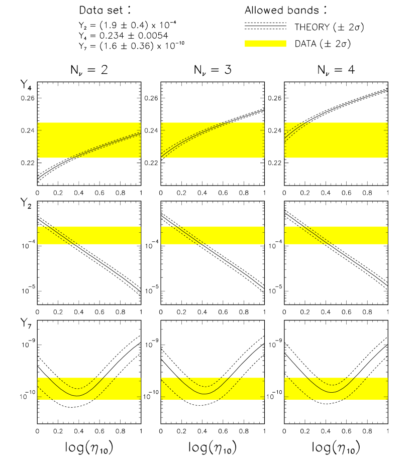
  Figure 4: Primordial abundances $Y_{4}$ (⁴He mass fraction) $Y_{2}$ (D/H) and $Y_{7}$ (⁷Li/H), for $N_{\nu}=2$, 3, and 4. Solid and dashed curves represent the theoretical central values and the $\pm 2\sigma$ bands, respectively. The grey areas represent the $\pm 2\sigma$ experimental bands for the data set A [18].

  

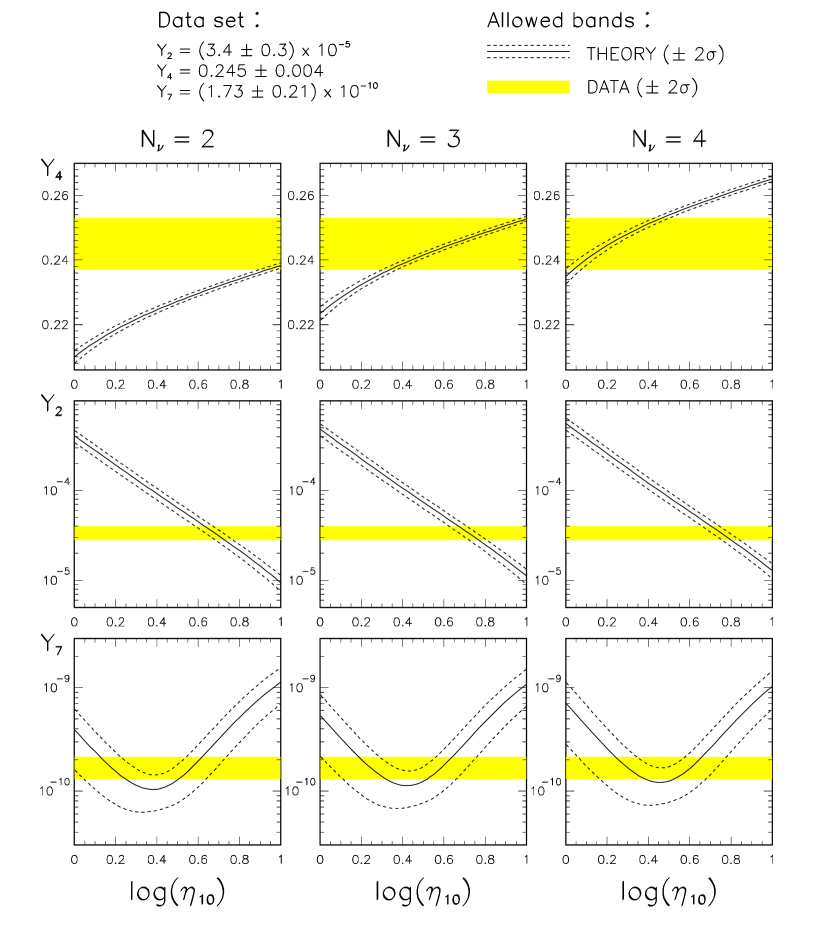
  Figure 6: Same as in figure 4, but for data set B [18].

  Figure 4 shows the abundances for various $N_{\nu}$ compared for illustration with data set A. While there is consistency between theory and data for $x\sim 0.2-0.4$ and $N_{\nu}=3$, for $N_{\nu}=2$ ($N_{\nu}=4$) the $Y_{2}$ data prefer values of $x$ lower (higher) than the $Y_{4}$ data. Therefore, we expect that a global fit will favor values of $(x,N_{\nu})$ close to $(0.3,3)$. Similarly, a fit to data set B should favour values of $(x,N_{\nu})\sim(0.7,3)$ as seen in figure 6.

  To quantify this we show in figure 8 the results of joint fits using the abundances of data set A. The abundances $Y_{2}$, $Y_{4}$, and $Y_{7}$ are used separately (upper panels), in combinations of two (middle panels), and all together, without and with the Ly$\alpha$-forest constraint on $\eta$ (lower panels). In this way the relative weight of each piece of data in the global fit can be understood at glance. The three C.L. curves (solid, thick solid, and dashed) are defined by $\chi^{2}-\chi^{2}_{\rm min}=2.3,\,6.2$, and $11.8$, respectively, corresponding to 68.3%, 95.4%, and 99.7% C.L. for two degrees of freedom ($\eta$ and $N_{\nu}$), i.e., to the probability intervals often designated as 1, 2, and 3 standard deviation limits. The $\chi^{2}$ is minimized for each combination of $Y_{i}$, but the actual value of $\chi^{2}_{\rm min}$ (and the best-fit point) is shown only for the relevant global combination $Y_{2}+Y_{4}+Y_{7}(+{\rm Ly}\alpha)$. For this data set, the helium and deuterium abundances dominate the fit, as can be seen by comparing the combinations $Y_{2}+Y_{4}$ and $Y_{2}+Y_{4}+Y_{7}$. The preferred values of $x$ are relatively low, and the preferred values of $N_{\nu}$ range between 2 and 4. Although the fit is excellent, the low value of $x$ is in conflict with the Ly$\alpha$-forest constraint on $\eta$, as indicated by the increase of $\chi^{2}_{\min}$ from 0.02 to 8.89.

  

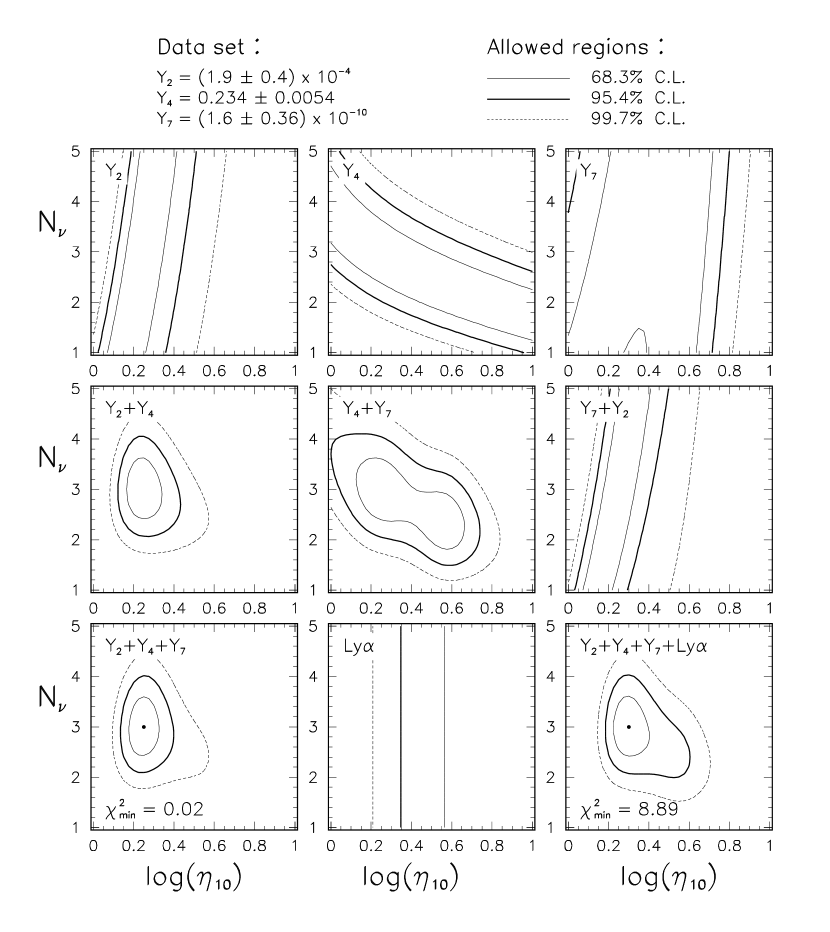
  Figure 8: Joint fits to $x=\log(\eta_{10})$ and $N_{\nu}$ using the abundances of data set A [18]. The abundances $Y_{2}$, $Y_{4}$, and $Y_{7}$ are used separately (upper panels), in combinations of two (middle panels), and all together, without and with the Ly$\alpha$-forest constraint on $\eta$ (lower panels).

  As shown in figure 10 there is no such problem with data set B which favors high values of $x$ because of the ‘low’ deuterium abundance. The combination of $Y_{2}+Y_{7}$ isolates, at high $x$, a narrow strip which depends mildly on $N_{\nu}$. The inclusion of $Y_{4}$ selects the central part of such strip, corresponding to $N_{\nu}$ between 2 and 4. As in figure 8, the combination $Y_{4}+Y_{7}$ does not appear to be very constraining. The overall fit to $Y_{2}+Y_{4}+Y_{7}$ is acceptable but not particularly good, mainly because $Y_{2}$ and $Y_{7}$ are only marginally compatible at high $x$. On the other hand, the $Y_{2}+Y_{4}+Y_{7}$ bounds are quite consistent with the Ly$\alpha$-forest constraint.

  

  Figure 10: Same as in Fig. 8, but for the data set B [18].

  Elsewhere [18] we have presented results for other possible combinations of input abundances. As shown in figure 12 (cf. [20]), one can also consider orthogonal combinations to those above, e.g. ‘high’ deuterium and ‘high’ helium, or ‘low’ deuterium and ‘low’ helium. The latter combination implies $N_{\nu}\sim 2$, thus creating the so-called “crisis” for standard nucleosynthesis [57]. Conversely, the former combination suggests $N_{\nu}\sim 4$, which would also constitute evidence for new physics. Allowing for depletion of the primordial lithium abundance to its Pop II value, relaxes the upper bound on $N_{\nu}$ further, as was noted earlier [59].

  

  Figure 12: The $68\%$ (solid) and $95\%$ (dotted) likelihood contours for the number of neutrino species and the nucleon-to-photon ratio, for all four combinations of the ‘high’ and ‘low’ deuterium and helium abundance measurements in data sets A and B.

  7 Conclusions

  It is clear from the above discussion that the present observational data on the primordial elemental abundances are not as yet sufficiently stable to derive firm bounds on $\eta$ and $N_{\nu}$. Different and arguably equally acceptable choices for the input data sets lead to very different predictions for $\eta$, and to relatively loose constraints on $N_{\nu}$ in the range 2 to 4 at the 95% C.L. Thus it may be premature to quote restrictive bounds based on some particular combination of the observations, until the discrepancies between different estimates are satisfactorily resolved. Our method of analysis provides the reader with an easy-to-use technique [11] to recalculate the best-fit values as the observational situation evolves further.

  

  Figure 14: Individual contributions of different reaction rates $R_{k}$ to the uncertainties in $Y_{2}$, $Y_{4}$, and $Y_{7}$, normalized to the corresponding total errors $\sigma_{2}$, $\sigma_{4}$, and $\sigma_{7}$, for $\eta=1.78\times 10^{-10}$, the best-fit value for data set A [17]. Each arrow corresponds to the shift $\delta\,Y_{i}$ induced by a $+1\sigma$ shift of $R_{k}$. Some small error components have not been plotted.

  

  Figure 16: Same as in figure 14, but for $\eta=5.13\times 10^{-10}$, the best-fit value for data set B [17].

  In order to improve the theoretical predictions further it is necessary to know the nuclear reaction rates better. To determine which reaction is largely responsible for the uncertainty in a particular elemental abundance (for any given nucleon density) is clearly important in this regard. In our approach this can be easily determined by “perturbing” the values of the input reaction rates and observing their effect on the predicted abundances, namely one can study the contribution to the total uncertainty $\sigma_{i}$ of $Y_{i}$ induced by a $+1\sigma$ shift of $R_{k}$:

  $$R_{k}\to R_{k}+\Delta\,R_{k}\ \Longrightarrow\ Y_{i}\to Y_{i}+\delta\,Y_{i}\ .$$ (34)

  We choose two particular values of $\eta$, $1.78\times 10^{-10}$ and $5.13\times 10^{-10}$, corresponding to the best-fit values for data sets A and B respectively and show in figures 14 and 16 the deviations $\delta\,Y_{i}$ (normalized to the total error $\sigma_{i}$) induced by $+1\sigma$ shifts in the $R_{k}$’s, plotted in the same set of planes as used for figure 2. The $1\sigma$ error ellipses shown in these figures are obtained by combining the deviation vectors $\delta Y_{i}/\sigma_{i}$ in an uncorrelated manner. Several interesting conclusions can be drawn from this exercise. As expected, the uncertainty in the weak interaction rate $R_{1}$ has the greatest impact on $Y_{4}$ for the high value of $\eta$ (figure 16), since essentially all neutrons end up being bound in ⁴He. However at the lower value of $\eta$ (figure 14), the uncertainty in $R_{2}$ — the “deuterium bottleneck” — plays an equally important role as $R_{1}$ in determining $Y_{4}$ because nuclear burning is less complete here than at high $\eta$. Similarly with reference to the reaction rates $R_{7}$, $R_{10}-R_{12}$ which synthesize ⁷Li, at low $\eta$ it is the competition between $R_{7}$ and $R_{11}$ which largely determines $Y_{7}$, while at high $\eta$ it is the competition between $R_{10}$ and $R_{12}$. The anticorrelation between $Y_{4}$ and $Y_{2}$ is driven mainly by $R_{2}$ at low $\eta$ and, to a lesser extent, by $R_{4}$ and $R_{5}$, while the reverse is the case at high $\eta$. The anticorrelation between $Y_{4}$ and $Y_{7}$ at low $\eta$ is also basically driven by $R_{2}$, while the correlation at high $\eta$ is due to both $R_{2}$ and $R_{4}$. Thus we have a direct visual basis for assessing in what direction the output abundances $Y_{i}$ are pulled by possible changes in the input cross sections $R_{k}$. This should be helpful in determining experimental strategies to determine key reaction rates more precisely.

  However one might ask what would happen if these discrepancies remain? We have already noted the importance of an independent constraint on $\eta$ (from the Ly$\alpha$-forest) in discriminating between different options. However, given the many assumptions which go into the argument [46], this constraint is rather uncertain at present. Fortunately it should be possible in the near future to independently determine $\eta$ to within $\sim 5\%$ through measurements of the angular anisotropy of the cosmic microwave background (CMB) on small angular scales [60], in particular with data from the all-sky surveyors MAP and PLANCK [61]. Such observations will also provide a precision measure of the relativistic particle content of the primordial plasma. Hopefully the primordial abundance of ⁴He would have stabilized by then, thus providing, in conjunction with the above measurements. a reliable probe of a wide variety of new physics and astrophysics which can affect nucleosynthesis (for recent work see [62, 63, 64, 65, 66, 67]).

  Acknowledgments

  It is a pleasure to thank Laura Baudis and Hans Klapdor-Kleingrothaus for organizing this enjoyable meeting, and my collaborators on BBN, Eligio Lisi and Francesco Villante, for allowing me to present our unpublished results.

References

- [1] Wagoner R V, Fowler W A and Hoyle F 1967 Astrophys. J. 148 3
- [2] Wagoner R V 1973 Astrophys. J. 179 343
- [3] Schramm D N and Turner M S 1998 Rev. Mod. Phys. 70 303
- [4] Steigman G 1998 astro-ph/9803055
- [5] Olive K A 1999 astro-ph/9901231
- [6] Sarkar S 1996 Rep. Prog. Phys. 59 1493
- [7] Sarkar S 1997 Dark Matter in Astro- and Particle Physics, ed H V Klapdor-Kleingrothaus and Y Ramachers (Singapore: World Scientific) p 235
- [8] Bernstein J A, Brown L S and Feinberg G 1989 Rev. Mod. Phys. 61 25
- [9] Esmailzadeh R, Starkman G D and Dimopoulos S 1991 Astrophys. J. 378 504
- [10] Kawano L 1992 Fermilab-Pub-92/04-A (unpublished)
- [11] http://www-thphys.physics.ox.ac.uk/users/SubirSarkar/bbn.html
- [12] Lopez R E and Turner M S 1998 astro-ph/9807279
- [13] Esposito S, Mangano G, Miele G and Pisanti O 1999 Nucl. Phys. B540 3
- [14] Caso C et al 1998 Eur. J. Phys. C3 1
- [15] Smith M S, Kawano L and Malaney R A 1993 Astrophys. J. Suppl. 85 219
-
[16]
Kernan P and Krauss L M 1994
Phys. Rev. Lett. 72 3309
Krauss L M and Kernan P 1995 Phys. Lett. 347 347 - [17] Fiorentini G, Lisi E, Sarkar S and Villante F L 1998 Phys. Rev. D58 063506
- [18] Lisi E, Sarkar S and Villante F L 1999 hep-ph/9901404
- [19] Olive K A and Thomas D 1997 Astropart. Phys. 7 27
- [20] Holtman E, Kawasaki M, Kohri K and Moroi T 1998 hep-ph/9805405.
- [21] Burles S, Nollett K M, Truran J N and Turner M S 1999 astro-ph/9901157
- [22] Eadie W T, Drijard D, James F E, Roos M and Sadoulet B 1971 Statistical Methods in Experimental Physics (Amsterdam: North Holland)
-
[23]
http://www.astro.washington.edu/mendoza/java/bbn
(will move to http://www.astro.washington.edu/bbn/) - [24] Pagel B E J 1997 Nucleosynthesis and the Chemical Evolution of Galaxies (Cambridge: Cambridge University Press)
- [25] Hogan C 1998 Sp. Sci. Rev. 84 127
- [26] Molaro P 1997 From Quantum Fluctuations to Cosmological Structures, ASP Conf. Ser. 126 103; private communication
-
[27]
Songaila A, Cowie L L, Hogan C J and Rugers M 1994
Nature 368 599
Carswell R F, Rauch M, Weymann R J, Cooke A J and Webb J K 1994 Mon. Not. R. Astr. Soc. 268 L1 - [28] Rugers M and Hogan C J 1996 Astron. J. 111 2135
-
[29]
Webb J K, Carswell R F, Lanzetta K M, Ferlet R, Lemoine M and
Vidal-Madjar A 1997
Nature 388 250
Tytler D, Burles S, Lu L, Fan X-M, Wolfe A and Savage B D 1998 astro-ph/9810217 -
[30]
Tytler D, Fan X-M and Burles S 1996
Nature 381 207
Burles S and Tytler D 1998 Astrophys. J. 499 699; 507 732; Sp. Sci. Rev. 84 65 -
[31]
Pagel B E J, Simonson E A, Terlevich R J and Edmunds M G 1992
Mon. Not. R. Astr. Soc. 255 325
Olive K A and Steigman G 1995 Astrophys. J. Suppl. 97 49 - [32] Olive K A, Steigman G and Skillman E D 1997 Astrophys. J. 483 788
- [33] Izotov Y I, Thuan T X and Lipovetsky V A 1994 Astrophys. J. 435 647; 1997 Astrophys. J. Suppl. 108 1
- [34] Izotov Y I and Thuan T X 1998 Astrophys. J. 497 227, 500, 188
- [35] Thorburn J A 1994 Astrophys. J. 421 318
- [36] Molaro P, Primas F and Bonifacio P 1995 Astron. Astrophys. 295 L47
- [37] Bonifacio P and Molaro P 1997 Mon. Not. Roy. Astron. Soc. 285 847
- [38] Ryan S G, Norris J E and Beers T C 1998 Astrophys. J. 506 892
- [39] Pinsonneault M H, Deliyannis C P and Demarque P 1992 Astrophys. J. Suppl. 78 179
- [40] Vauclair S and Charbonnel C 1995 Astron. Astrophys. 295 715; 1998 Astrophys. J. 502 372
- [41] Bonifacio P and Molaro M 1998 Astrophys. J. Lett. 500 L175
- [42] Jedamzik K and Fuller G M 1996 Astrophys. J. 483 560
- [43] Burles S, Kirkman D and Tytler D 1996 astro-ph/9612121
-
[44]
Levshakov S A, Kegel W H and Takahara F 1998
Astrophys. J. 499 L1
Levshakov S A, Tytler D and Burles S 1998 astro-ph/9812114 - [45] Pinsonneault M H, Walker T P, Steigman G and Naranyanan V K 1998 astro-ph/9803073
- [46] Weinberg D H, Miralda-Escudé J, Hernquist L and Katz N 1997 Astrophys. J. 490 564
-
[47]
Persic M and Salucci P 1992
Mon. Not. R. Astr. Soc. 258 14p
Fukugita M, Hogan C J and Peebles P J E 1998 Astrophys. J. 503 518 - [48] Conrad J 1998 hep-ex/9811009
-
[49]
Hoyle F and Tayler R J 1964
Nature 203 1108
Peebles P J E 1966 Phys. Rev. Lett. 16 411
Shvartsman V F 1969 JETP Lett. 9 184 -
[50]
Steigman G, Schramm D N and Gunn J 1977
Phys. Lett. 66B 202
Steigman G, Olive K A and Schramm D N 1979 Phys. Rev. Lett. 43 239 - [51] Olive K A, Schramm D N and Steigman G 1981 Nucl. Phys. B180 497
- [52] Enqvist K, Kainulainen K and Thomson M 1992 Nucl. Phys. B373 498
-
[53]
Kirilova D P and Chizhov M V 1998
Nucl. Phys. B534 447
Foot R and Volkas R R 1997 Phys. Rev. D55 5147 -
[54]
Dolgov A D, Hansen S H, Pastor S and Semikoz D V 1998
hep-ph/9809598
Hannestad S 1998 Phys. Rev. D57 2213
Kawasaki M, Kohri K and Sato K 1998 Phys. Lett. B430 132 - [55] Dolgov A D, Pastor S, Romão J C and Valle J W F 1997 Nucl. Phys. B496 24
-
[56]
Yang J, Turner M S, Steigman G, Schramm D N and Olive K A 1984
Astrophys. J. 281 493
Steigman G, Olive K A, Schramm D N and Turner M S 1986 Phys. Lett. B176 33
Olive K A, Schramm D N, Steigman G and Walker T P 1990 Phys. Lett. B236 454
Walker T P, Steigman G, Schramm D N, Olive K A and Kang H-S 1991 Astrophys. J. 376 51 - [57] Hata N, Scherrer R J, Steigman G, Thomas D, Walker T P, Bludman S and Langacker P 1995 Phys. Rev. Lett. 75 3977
- [58] Ellis J, Enqvist K, Nanopoulos D V and Sarkar S 1986 Phys. Lett. B167 457
- [59] Kernan P J and Sarkar S 1996 Phys. Rev. D54 R3681
-
[60]
Knox L 1995
Phys. Rev. D52 4307
Jungman G, Kamionkowski M, Kosowski A and Spergel D N 1996 Phys. Rev. D54 1332
Zaldarriaga M, Spergel D N and Seljak U 1997 Astrophys. J. 488 1
Bond J R, Efstathiou G and Tegmark M 1997 Mon. Not. R. Astron. Soc. 291 L33 -
[61]
MAP: http://map.gsfc.nasa.gov/
PLANCK: http://astro.estec.esa.nl/SA-general/Projects/Planck/ - [62] Bell N F, Foot R and Volkas R R 1998 Phys. Rev. D58 105010
- [63] Damour T and Pichon B 1998 astro-ph/9807176
- [64] Gherghetta T, Giudice G F and Riotto A 1998 hep-ph/9808401
- [65] Kainulainen K, Kurki-Suonio H and Sihvola E 1998 astro-ph/9807098
- [66] Mohapatra R N and Teplitz V L 1998 Phys. Rev. Lett. 81 3079
- [67] Rehm J B and Jedamzik K 1998 Phys. Rev. Lett. 81 3307