Effective Radii and Color Gradients in Radio Galaxies

Abstract

We present de Vaucouleurs’ effective radii in $B{\rm\ and\ }R$ bands for a sample of Molonglo Reference Catalogue radio galaxies and a control sample of normal galaxies. We use the ratio of the scale lengths in the two bands as an indicator to show that the radio galaxies tend to have excess of blue color in their inner region much more frequently than the control galaxies. We show that the scale length ratio is a useful indicator of radial color variation even when the conventional color gradient is too noisy to serve the purpose.

1 Introduction

Traditionally, radio galaxies were believed to be ellipticals consisting of a coeval population of old stars, and almost no dust or gas. However, detailed photometric studies in the optical band, as well as X-ray observations, have demonstrated that elliptical galaxies, especially those hosting radio sources, not only have significant quantities of dust and gas, but also possess fine morphological structure indicating some amount of activity in the past $\sim 10^{2}$ million years (see e. g.  Smith & Heckman 1989). Radio galaxies host an active galactic nucleus (AGN) and also have radio jets which transport a very large amount of energy over hundreds of kiloparsecs. Such phenomena are likely to be associated with morphological features and star formation activity not found in normal elliptical galaxies.

In this paper we present the main results from a detailed morphological study of a sample of radio galaxies from the Molonglo Reference Catalogue (MRC). We present de Vaucouleurs’ effective radii (scale lengths), obtained from careful model fits to surface brightness profiles of the galaxies, and show that the ratio $r_{e}(B)/r_{e}(R)$, of the scale lengths in $B{\rm\ and\ }R$ filters, provides a measure of the color gradient in the galaxy. The ratio is related to color gradients measured conventionally, but is more robust: it can provide an estimate of the color gradient even when the signal-to-noise ratio is not good enough for the color gradient to be measured unambiguously using the conventional technique. Using the ratio we show that a large fraction of radio galaxies become bluer towards the center.

2 Sample and observations

Our results are based on the observations of 30 galaxies from the MRC which have $408\,{\rm MHz}$ radio flux $S_{408}>0.95\,{\rm Jy}$, redshift $z<0.3$ and declination $-30\deg\leq\delta(1950)\leq-20\deg$. The objects were observed from the Las Campanas Observatory (LCO), Chile in Jan 1995 and Feb 1996 using the 1.0m f/7 Swope telescope and the 2.5m f/7.5 Du Pont telescope. Images were obtained in Johnson’s $B$ and Cousin’s $R$ filters, which are centered at $0.44\micron$ and $0.65\micron$ respectively and have a bandwidth of $\sim 0.1\micron$. The typical exposure time was $\sim 20\min$ in $R$ and $\sim 60\min$ in $B$. The FWHM of the PSF ranged from $\sim 1^{\prime\prime}\!.1$ to $\sim 1^{\prime\prime}\!.5$. When the FWHM of the PSF was different for the images in $B{\rm\ and\ }R$ filters for the same object, the better PSF was degraded to match the other before it was used to compare properties that involve both the filters. The plate scale was $0^{\prime\prime}.7/\,{\rm pixel}$ and the total field of view covered in an exposure was $11^{\prime}.5\times 11^{\prime}.5$ in Jan 1995 and $23^{\prime}\times 23^{\prime}$ in Feb 1996. The large field allowed us to determine the sky background more accurately than is usually possible. All the processing was done in the normal way using tasks from IRAF and STSDAS, and the details will be published elsewhere (Mahabal, Kembhavi & McCarthy 1999).

For the purpose of comparison we extracted a control sample from the CCD fields of our radio galaxies. The sample consists of all non-radio, early type galaxies from the fields which have semi-major axis length $>\,15^{\prime\prime}$. There are 30 galaxies in the control sample, and these were processed and analyzed in a fashion identical to the radio galaxies. The redshifts for the galaxies in the control sample are not known. However, the distribution of angular sizes and apparent magnitudes for the control sample are similar to that of the radio sample and hence the redshift distributions for the two samples are unlikely to be too different. Our main results, based on the ratio of scale lengths in the $B{\rm\ and\ }R$ filters are unlikely to be affected by any small changes in the redshift distribution.

3 Surface photometry

We fitted the isophotes of each galaxy in both $B{\rm\ and\ }R$ filters with a succession of ellipses with different semi-major axis lengths using tasks in IRAF based on the algorithm described by Jedrzejewski (1987). The mean surface brightness for the series of best-fit ellipses gives us the radial surface brightness profile of a galaxy as a function of semi-major axis length. From the radial profile in the two bands we obtained the $B-R$ color profile for each galaxy.

Major contributions to the galaxian light can in general come from a spheroidal bulge and a flattened disk. In active galaxies an additional substantial contribution to the central region can be made by the active galactic nucleus (AGN) acting as a point source. The relative strengths of the components vary over galaxy type, and can be determined by fitting the observed radial surface brightness profile of the galaxy with a composite model made up of contributions from each component.

We have assumed that the bulge profile is described by de Vaucouleurs’ law, and the disk profile by an exponential. The contribution of the AGN corresponds to a point source broadened by the point spread function. We have found for our sample of radio galaxies that the AGN is too weak to be unambiguously detected, and distinguished from other compact features which may be present. We therefore do not include an AGN in our fits. The model surface brightness $I(r)$ at semi-major axis length $r$ is then given by

$$I(r)=I_{e}\exp\{-7.67[(r/r_{e})^{1/4}-1]\}+I_{d}\exp(-r/r_{d})$$ (1)

where $I_{e}$ is the bulge intensity at de Vaucouleurs’ effective radius (scale length) $r_{e}$, $I_{d}$ is the disk surface brightness at $r=0$, and $r_{d}$ is the disk scale-length. de Vaucouleurs’ law is known to provide a good fit over the range $0.1r_{e}<r<1.5r_{e}$ (Burkert 1993). The points that we use in our fits lie in this range.

To obtain the best-fit model to an observed galaxy profile, we generate a model galaxy with two dimensional surface brightness distribution corresponding to trial values of the four parameters in Equation 1, and observed bulge and disk ellipticities. We convolve the model with a Gaussian point-spread function (PSF) determined from the observed frames for the galaxy in question, and then obtain the model radial profile. We determine the best-fit parameters by minimizing the reduced chi-square function $\chi^{2}_{\nu}=\sum(I_{o}-I_{m})^{2}/\nu\sigma^{2}$, where $I_{0}$ and $I_{m}$ are the observed and model surface brightnesses at specific distances along the semi-major axis. The standard deviation $\sigma$ at each point is obtained from the ellipse fitting task in IRAF and includes photon counting as well as ellipse fitting errors; $\nu$ is the number of degrees of freedom, and is equal to the number of points used in the fit reduced by the number of free parameters.

Contributions to $\chi^{2}_{\nu}$ are obtained at semi-major axis lengths $r$ in the range $r_{1}<r<r_{2}$, where the inner limit $r_{1}$ is chosen such that it lies at a radial separation of 1.5 times the full width at half maximum (FWHM) of the PSF and the outer limit $r_{2}$ is chosen where $\sigma(I)/I$ drops to 0.1. We have omitted points inside $r_{1}$, which typically involve just a few pixels, from the fit because the profile here can be seriously affected by the PSF, as well as by any departures from de Vaucouleurs’ law that may be present close to the center. The PSF influences the shape of the profile to several times the FWHM (see Franx, Illingworth, & Heckman 1989; Peletier et al. 1990), but we account for this in our work by convolving the model profile with a model PSF before comparing it with the observed profile. We have carried out runs on artificial galaxies (created using the IRAF package artgal) and on nearby elliptical galaxies and galaxies from our sample which suggest that the value of the extracted effective radius stabilizes beyond 1.5 times the PSF FWHM (Mahabal 1998), when PSF convolved profiles are used.

We have fitted the bulge plus disk combination in Equation 1 to the radio galaxies. In many cases the ratio $D/B$ of the disk to bulge luminosity is $\ll 1$, which is consistent with the radio galaxies being ellipticals. In some cases we detect a disk component $D/B\geq 0.3$, but the disk scale length is small, except in two cases, so that the detected “disk” is a small scale structure unlike the disks in spiral galaxies. We will describe elsewhere our findings regarding the disk like structures, and devote our attention here to the bulges. Pure bulge fits also turn out to be acceptable in most cases, but the disk plus bulge fits provide better $\chi^{2}_{\nu}$ values on the whole, and we retain them as one of our aims in the larger investigation has been to find any disk like structures which may be present. The results reported here would not change if pure bulge fits were used in the discussion. None of the control galaxies has a significant disk component.

3.1 Goodness of fit

We get very good ($\chi^{2}_{\nu}<1$) or acceptable ($1<\chi^{2}_{\nu}<2$) fits in $\sim 85\%$ of the cases for the radio as well as the control sample. Visually too $<\sim 10\%$ galaxies are seen to be highly distorted in the radio sample. It follows that strong radio sources do not prefer highly distorted galaxies. $\chi^{2}_{\nu}$ does not increase as a function of redshift, i. e.,  we get good fits right upto the redshift of 0.3 that we have considered. We find that $\chi^{2}_{\nu}(B)$ values are in general smaller than the corresponding $\chi^{2}_{\nu}(R)$ values. The lower values in $B$ are partly due to the higher $\sigma$ values there. It also appears that isophote distorting influences like emission and absorption regions which could increase $\chi^{2}_{\nu}(B)$ are averaged out in the ellipse and profile fits.

Figure 1: $r_{e}$ in $B{\rm\ and\ }R$ filters for the radio sample (left) and the control sample (right). The dotted line is the locus $r_{e}(B)=r_{e}(R)$. Points above it denote galaxies which become bluer inwards. There is a larger number of such cases amongst the radio galaxies.

3.2 Bulge parameters

We now turn to the bulge scale lengths. 1 shows a plot of $r_{e}(B)$ against $r_{e}(R)$ for the radio and control galaxies. The $1\sigma$ errors on $r_{e}$, obtained from the fitting program, are typically $\sim 10\%$. The scale lengths in the two filters are equal to within $1\sigma$ in several cases, and these values are scattered around the $r_{e}(B)=r_{e}(R)$ line in the figure. In the other cases we have $r_{e}(B)<r_{e}(R)$ (points above the equality line) or $r_{e}(B)>r_{e}(R)$ (points below). It is obvious from the figure that the former are more numerous in the radio galaxies, while the latter occur more frequently in the control galaxies.

When $r_{e}(B)>r_{e}(R)$, the surface brightness in $R$ increases more rapidly towards the center than the surface brightness in B. In other words, from the definition of the effective radius $r_{e}$, half the red light from the galaxy is contained in a smaller region than half the blue light. $r_{e}(B)>r_{e}(R)$ therefore implies that the galaxy on the average becomes redder inwards. Similarly, when $r_{e}(B)<r_{e}(R)$, the galaxy becomes bluer as one moves towards the center. The distribution of points in 1 therefore show that the radio galaxies become bluer towards the center more often than the control galaxies.

We have shown in 2 the distribution of the ratio $r_{e}(B)/r_{e}(R)$ for the radio and control galaxies. An application of the Kolmogorov-Smirnov test shows that the two distributions are different at 99.99% confidence level. For the radio sample the mean value of the ratio is $\left<r_{e}(B)/r_{e}(R)\right>_{r}=0.87\pm 0.15$, while for the control sample the mean value is $\left<r_{e}(B)/r_{e}(R)\right>_{c}=1.25\pm 0.10$. The larger value of the ratio for the control sample is consistent with previous studies of early type galaxies, which showed that their colors become redder inwards (e. g.  Sandage & Vishwanathan 1978). Contrary to this behavior, the distribution of the bulge scale length ratio for the radio galaxies shows that they tend to become bluer as one moves towards their inner region, i. e.,  the color variation in radio galaxies is opposite of that in the control galaxies. In the next section we will consider the relation between the scale length ratio and the conventional color gradient.

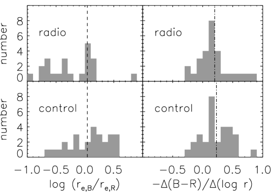
Figure 2: The distribution of $r_{e}(B)/r_{e}(R)$ (left) and the color gradient (right) for the radio and control samples. Negative numbers on the x-axis are indicative of galaxies with excess blue emission towards the center.

We have excluded from the profile fits points within 1.5 times the FWHM of the PSF from the center. For our sample the excluded region has a physical dimension extending to $\sim 4\,{\rm kpc}$ at the highest redshift. It follows that the inner bluer color of the radio galaxies is not due to a blue AGN or other unresolved features at the center, and must arise in regions which are spread out.

4 Color gradients

The color variation in a galaxy is normally measured by a color gradient parameter $G\equiv\Delta(B-R)/\Delta({\rm log\,r})$. The change in color per decade in radius is almost linear in most galaxies and $G$ is obtained by fitting a straight line to the color profile between an inner radius $r_{1}$ and an outer radius $r_{2}$. We choose these radii as described in Section 3, with the additional caveat that now $r_{2}=\min{(r_{2}(B),r_{2}(R))}$.

When two small galaxies (angular diameter $<15^{\prime\prime}$) and a quasar host in our radio sample are excluded, we find that the mean color gradients, in magnitudes per $\,{\rm arcsec^{2}}$ per decade in radius, for the radio and control samples are $\left<G\right>_{r}=-0.20\pm 0.05$ and $\left<G\right>_{c}=-0.23\pm 0.05$. The distribution of gradients is shown in 2. We find that the numbers that we obtain are larger in magnitude than those obtained by other authors. For a sample of normal ellipticals (with dusty galaxies excluded) Peletier et al.  (1990) had obtained a color gradient of –0.1. Zirbel (1996) had obtained a value of –0.15 for a sample of radio galaxies. However, we have confirmed that the larger numbers we get are not owing to photometric errors.

4.1 Color gradients and scale length ratios

Color gradients and scale length ratios are both indicative of the change in color with distance from the center and they are related, to a first approximation, by:

$$G\equiv\frac{\Delta(B-R)}{\log r_{2}/r_{1}}\simeq\frac{2.06(r_{2}^{1/4}-r_{1}^{1/4})}{r_{e}(B)^{1/4}\log(r_{2}/r_{1})}\left(1-\frac{r_{e}(B)}{r_{e}(R)}\right).$$ (2)

For galaxies that obey de Vaucouleurs’ law the color gradient can therefore be estimated from the fitted bulge scale lengths. We enumerate in Table 1 the distribution of color gradients obtained using the scale lengths, as well as the gradients obtained directly from the color profiles using the measured values of the $B-R$ color at $r_{1}$ and $r_{2}$ We have deviated from the more usual custom of taking the outer point at $r_{e}$ since in some cases the color profile is very noisy at that radius. The gradient does not change very much with changes in $r_{1}$ and $r_{2}$. It is seen from the table that the color gradients obtained directly from the color profiles have a different distribution from the bulge scale length related color gradient. The distribution of the latter clearly shows that radio galaxies become bluer towards the center while the control galaxies become redder. This distinction is not obvious from the distribution of the directly measured color gradient. In 3 we have plotted the conventional color gradient against that obtained from the scale lengths for the radio galaxies. A simple $2\times 2$ contingency test shows that the two color indicators vary in the same sense.

Color	From color profile		From scale lengths
gradient	Radio	Control	Radio	Control
$<0$	20	24	9	20
$>0$	7	6	18	10
uncertain	3	0	3	0

Table 1: Color gradient details for the two samples as obtained from the color profile and from the bulge scale lengths. A negative color gradient is indicative of a redder center relative to the outer regions.

Figure 3: Conventional color gradient against color variation as given by the $B{\rm\ and\ }R$ scale lengths for the radio galaxies. The latter is indicative of bluer central regions in many cases. A $2\times 2$ contingency test shows that the two color indicators vary in the same sense.

Figure 4: Top: correlation of dust mass in radio galaxies with dust lanes (filled diamonds) or dust patches (open diamonds) at the center with radio power. Bottom: $r_{e}(B)/r_{e}(R)$ as a function of radio power. The dashed line shows the scale length ratio expected for a normal galaxy. There is a hint that more powerful galaxies are bluer towards the center.

The conventional color gradient is obtained by fitting a straight line to the color profile, which neglects any curvature that may be present. Also, due to the limited signal-to-noise available, often the errors on the color gradient can be large, making the measured values uncertain. The process of obtaining scale lengths involve averaging over isophotes as well as the profile fit with an empirically tested model. We have seen above that the $\chi^{2}_{\nu}$ obtained are well within acceptable limits in most cases for good fits. The scale lengths are therefore good, robust indicators of the large scale distribution of light in the galaxy, and their ratio in the two filters provides a useful descriptor of the way the color changes over the galaxy. Using the ratio we have demonstrated the ubiquity of inner blue color in radio galaxies, a fact which is not apparent from the conventional color gradient.

4.2 Discussion

Color gradients in early type galaxies are believed to be due to metallicity and age gradients in the stellar population. The presence of dust produces increased reddening, while star formation leads to bluer colors. In addition to any overall color gradient that we observe in the radio galaxies, their $B-R$ color images show regions of excess reddening indicative of dust. The dust occurs in the form of coherent lanes in $\sim 20\%$ of the galaxies, while another $\sim 17\%$ show dust patches. The remaining objects could of course contain dust well mixed with stars, which is not evident in the color maps. In several of the galaxies with $r_{e}(B)/r_{e}(R)>1$, we see clear clear evidence of dust in the color maps. In the control galaxies detectable dust again occurs in $\sim 37\%$ of the sample, but here the dust is more often patchy ($30\%$).

Assuming that the composition of dust in the radio sample is similar to that in our Galaxy, and by using a simple screen model with constant gas-to-dust ratio (see e. g. Burstein & Heiles 1978), the mass of the dust can be estimated in the usual manner from the excess $B-R$ color. The dust mass turns out to be in the range $\sim 10^{5}-10^{7}M_{\odot}$. A plot of dust mass against radio power (see 4) shows that the two are correlated, the linear correlation coefficient being significant at better than the $99\%$ confidence level. The dust mass as well as the luminosity depend on the square of the distance, which could lead to a false correlation. The distance effect is probably not serious in the present case since the partial correlation coefficient, obtained after factoring out the distance, remains significant at better than the $90\%$ level.

We have seen above that the distribution of the $r_{e}(B)/r_{e}(R)$ in the radio galaxies indicates that these objects more often become bluer towards the center than the control galaxies. The blue color is presumably due to star formation which is in some manner induced by the presence of the radio source. We have shown in 4 a plot of the logarithm of the total radio power at $408\,{\rm MHz}$ against $\log(r_{e}(B)/r_{e}(R))$. It is seen that there is a clear trend for the more powerful radio galaxies to have steeper color gradients as indicated by the scale length ratio. The more luminous a radio source is, the greater seems to be the increased blue luminosity triggered by it. Best, Longair, & Röttgering (1996) report finding either a string of bright star forming knots or compact knots in the case of $z\sim 1$ radio galaxies from the 3CR catalogue. These are thought to be produced by the interaction of the radio jet with the interstellar medium. It will be possible to model the mass and spatial extent of the gas involved in the bursts from narrow band imaging and long-slit spectra of the galaxies.

5 Conclusions

Using detailed model profile fits to the observed surface brightness profiles of samples of radio and control galaxies, we have shown that the distribution of the $r_{e}(B)/r_{e}(R)$ ratio is different for the two samples. A value $<1$ for this ratio in a galaxy indicates that the color of the galaxy becomes bluer towards the center, while $r_{e}(B)/r_{e}(R)>1$ indicates that the color becomes redder towards the center. The ratio has a simple relation with the color gradient $G$ obtained directly from color profiles. But the ratio can be used as an indicator of the radial dependence of color, even when the measured gradient is too noisy to serve the purpose.

References

- (1) Best, P. N., Longair, M. S., & Röttgering, H. J. A. 1996, MNRAS, 280, L9
- (2) Burkert, A. 1993, A&A, 278, 23
- (3) Burstein, D., & Heiles, C. 1978, ApJ, 225, 40
- (4) Franx, M., Illingworth, G., & Heckman, T. 1989, AJ, 98, 538
- (5) Jedrzejewski, R. I. 1987, MNRAS, 226, 747
- (6) Mahabal, A. A. 1998, PhD thesis, Pune University
- (7) Mahabal, A. A., Kembhavi, A. K., & McCarthy, P. J. 1999, (Submitted to ApJ)
- (8) Peletier, R. F., Davies, R. L., Davis, L. E., Illingworth, G. D., & Cawson, M. 1990, AJ, 100, 1091
- (9) Sandage, A., & Vishwanathan, N. 1978, ApJ, 223, 707
- (10) Smith, E. P., & Heckman, T. M. 1989, ApJ, 341, 658
- (11) Zirbel, E. 1996, ApJ, 473, 713