Stability of rotating spherical stellar systems

Abstract

We study the stability of rotating collisionless self-gravitating spherical systems by using high resolution N-body experiments on a Connection Machine CM-5.

We added rotation to Ossipkov-Merritt (hereafter OM) anisotropic spherical systems by using two methods. The first method conserves the anisotropy of the distribution function defined in the OM algorithm. The second method distorts the systems in velocity space. We then show that the stability of systems depends both on their anisotropy and on the value of the ratio between the total kinetic energy and the rotational kinetic energy. We also test the relevance of the stability parameters introduced by Perez et al. (1996) for the case of rotating systems.

1 Introduction

Various analytical and numerical studies [Antonov 1973, Barnes et al. 1986, Palmer & Papaloizou 1986, Perez & Aly 1996, Perez et al. 1996] (and references therein) have shown that spherical, collisionless, self-gravitating anisotropic systems with components moving mainly on radial orbits are unstable. However, all these works considered non-rotating systems, and it is well known that rotation can play an important role in the dynamical evolution of systems and modify their stability properties. It has been shown that rotation can be the cause of the deformation of systems like globular clusters or weakly elliptical galaxies [Goodwin 1997, Staneva et al. 1996].

The stability of rotating stellar systems is a very complex problem, Much work has been concerned with barred galaxies (which are rapidly rotating stellar systems) (for a review see, IAU Colloquium 157 ), but in a more general context, few studies have been devoted in the literature to this topic. For example, Papaloizou, Palmer and Allen (1991) have performed a series of numerical simulations to analyze the stability of systems where rotation was introduced by using the technique proposed by Lynden-Bell (1962). All their simulations produced endstates in which a triaxial bar appears. These important results cannot be considered general, since they were obtained for systems dominated by particles evolving on radial orbits, and was put in rotation by a specific procedure. In order to analyze the influence of rotation on the (in)stability of a given system, it is necessary to consider not only spherical systems with different kinds of anisotropy but also different methods for introducing the rotation. This paper develops such an analysis. We are also interested in testing the relevance of the stability parameters [Perez et al. 1996] on rotating systems. Perez et al. (1996) have shown that the stability of spherical self-gravitating non-rotating systems can be deduced from the ’anisotropic’ component of the linear variation of the distribution function (see below Section 2.2). Such stability parameters can be computed from rotating systems. We show that they are still relevant for anisotropic systems as long as the rotational kinetic energy is not too large.

The paper is arranged as follows. We describe in Section 2 the method that we use to obtain the initial non-rotating systems as well as the parameters describing the (in)stability of such systems. In Section 3, we detail the techniques used to introduce a parameterizable rotation to the initial conditions presented in Section 2. In Section 4, we show our numerical results on the (in)stability of various rotating systems generated with different procedures. Finally, the discussion and physical interpretation of our results are presented in Section 5.

2 Stability and Instability of Non-rotating Systems

2.1 Non-rotating Initial Conditions

In a previous paper [Perez et al. 1996], we used the OM algorithm [Ossipkov 1979, Merritt 1985a, Merritt 1985b, Binney & Tremaine 1987] to generate anisotropic self-gravitating spherical systems with various physical properties. This algorithm starts from a density given by $\rho_{\rm iso}(r)\propto\psi_{\rm iso}^{n}$, where $\psi_{\rm iso}(r)$ is a known gravitational potential satisfying the Poisson equation, while $n$ is the polytropic index ($1/2<n\leq 5$). This density profile $\rho_{iso}(r)$ is then deformed according to:

$$\rho_{\rm ani}(r)\;\;:=\;\;\left(1+\frac{r^{2}}{r_{\rm a}^{2}}\right)\rho_{\rm iso}(r)\,,$$ (1)

where the anisotropic radius $r_{\rm a}$ is a parameter which controls the deformation.

Using the Abel inversion technique, this procedure allows one to define an anisotropic distribution function (hereafter DF) which depends both on $E$ and $L^{2}$ through the variable $Q\;\;:=\;\;E+L^{2}/2r_{\rm a}^{2}$

$$f_{o}(Q)\;\;=\;\;\frac{\sqrt{2}}{4\pi^{2}}\frac{d}{dQ}\int_{Q}^{0}\frac{d\psi_{\rm iso}}{\sqrt{\psi_{\rm iso}-Q}}\;\frac{d\rho_{\rm ani}}{d\psi_{\rm iso}}\,.$$ (2)

Once this DF has been computed, the initial conditions of our N-body numerical simulations are generated by choosing at random, from the above DF, the positions and velocities for the $N$ particles. The density profile $\rho_{ani}(r)$ defined by equation 1 is the probability density from which the positions are generated. The velocities are generated from the velocity probability density deduced from the equation 2 (see appendix).

It must be noted that, there is a fundamental limitation in the OM models: Any given value of the polytropic index $n$ implies a critical value of $r_{a}$ below which the DF becomes negative and unphysical in some region of phase space. Merritt (1985a) interprets this limitation as a simple illustration of the well-known fact that radial orbits cannot always reproduce an arbitrary spherical mass distribution. In theses cases, in order to extend the OM algorithm to highly radially anisotropic ($r_{a}\simeq 1$) systems, we have arbitrarily set the DF equal to zero in this region. Such a procedure on DF affect only particles with a large value of $Q$. This procedure is applied for systems with a small value of $r_{a}$ which contains mainly particles with a small value of $Q$. Such a procedure affect then a very small number of particles (less than $0.1\%$ of the total number of particles). The systems with a modified DF are not strictly OM systems. However they conserve the properties which are for the present work: the density profils deduced from the modified DF are indistinguishable from the density profils given by equation (1) with the same value of $r_{a}$, the Lindblad diagrams are very peaked around a small value of $Q$ [Perez et al. 1996], they well correspond to highly radially anisotropic systems, and finally the radial dependence of the velocity anisotropy

$$\frac{\sigma_{r}^{2}}{\sigma_{t}^{2}}\;\;:=\;\;\frac{<v_{r}^{2}>}{\frac{1}{2}<v_{t}^{2}>}\;\;=\;\;1+\frac{r^{2}}{r_{a}^{2}}\,.$$ (3)

is preserved.

Finally, since each particle is initialized independently, the equilibrium DF $f_{o}(E,L^{2})$ of the system is in fact slightly perturbed. The perturbation is due to local Poissonian fluctuations of the density. The dynamical evolution of the system then represents the response of an anisotropic self-gravitating spherical equilibrium system submitted to such a perturbation.

2.2 Stability Analysis

The equilibrium DF of a spherical self-gravitating system depends only on the one-particle energy $E$ and the squared total angular momentum $L^{2}$. If $g_{1}$ denotes the perturbation generator, the linear variation of the DF can be written as

$$\delta f\;=\;\frac{\partial f_{o}}{\partial E}\{g_{1},E\}+\frac{\partial f_{o}}{\partial L^{2}}\{g_{1},L^{2}\}.$$ (4)

If DF is a monotonic decreasing function, the stability is then related to the Poisson brackets $\{g_{1},E\}$ and $\{g_{1},L^{2}\}$ [Perez & Aly 1996, Perez et al. 1996]. In our N-body simulations, these quantities appear as two random variables, $\epsilon$ and $\lambda$ respectively, defined for each particle $i$ [Perez et al. 1996]. The stability of the system can be predicted from the probability $P_{\epsilon}$ for $\epsilon$ to be negative, and the statistical Pearson index [Calot 1973] $P_{\lambda}$ of the variable $\lambda$. All anisotropic collisionless self-gravitating non-rotating spherical systems with

$$P_{\lambda}\la 2.5\;\mbox{and}\;P_{\epsilon}\ga 20\%$$ (5)

are unstable, while those with

$$P_{\lambda}\ga 2.5\;\mbox{and}\;P_{\epsilon}\la 20\%$$ (6)

are stable. The two other regions of the $(P_{\lambda}P_{\epsilon})$ plane, correspond to a transition between a stable system and an unstable system. In the particular case of OM models, these regions correspond to an anisotropy radius $r_{\rm a}$ close to 2 [Perez et al. 1996].

3 Generation of Rotating Systems

3.1 Definition

In order to generate virial-relaxed rotating spherical systems, we modify the non-rotating systems defined in the previous section by using techniques derived from the Lynden-Bell method (1962). Since this method preserves the position and the norm of the velocity of each particle, the systems are put in rotation without modifying their total potential and kinetic energy. In practice, we apply the following transformations to the velocity components $\{v_{r},v_{\theta},v_{\phi}\}$ of the particles:

$$\begin{array}[]{ll}Method\;1&Method\;2\\ v_{r}\longrightarrow v_{r}&v_{r}\longrightarrow 0.\\ v_{\theta}\longrightarrow v_{\theta}&v_{\theta}\longrightarrow v_{\theta}\\ v_{\phi}\longrightarrow\mid\!v_{\phi}\!\mid&v_{\phi}\longrightarrow\displaystyle{\sqrt{1+\frac{v_{r}^{2}}{v_{\phi}^{2}}}}\mid\!v_{\phi}\!\mid\end{array}$$ (7)

The first method then conserves the radial anisotropy defined in the OM algorithm, while the second method distorts the system in velocity space.

The amount of rotation introduced by these methods can be evaluated through the ratio:

$$\mu=K_{rot}/K_{tot},$$ (8)

where $K_{tot}$ is the total kinetic energy, and $K_{rot}$ is the rotation kinetic energy defined by Navarro and White (1993):

$$K_{rot}=\frac{1}{2}\sum_{i=1}^{N}m_{i}\frac{(\mbox{\bf\sl L}_{i}\cdot\hat{\mbox{\bf\sl L}}_{tot})^{2}}{[r_{i}^{2}-(\mbox{\bf\sl r}_{i}\cdot\hat{\mbox{\bf\sl L}}_{tot})^{2}]}$$ (9)

Here, L_i is the specific angular momentum of particle i, $\hat{\mbox{\bf\sl L}}_{tot}$ is a unit vector in the direction of the total angular momentum of the system, when the system does not rotate at all the $\hat{\mbox{\bf\sl L}}_{tot}$ vector is the null vector, and $N$ is the total number of particles. In order to exclude counter-rotating particles, the sum in equation (9) is actually carried out only over those particles satisfying the condition $(\mbox{\bf\sl L}_{i}\cdot\hat{\mbox{\bf\sl L}}_{tot})>0$.

In order to have systems with different strengths of homogeneous rotation (HR), we have applied either Method 1 or Method 2 to a fraction $\tau$ of the total number of particles. This fraction has been constructed by choosing the particles at random in the overall system. When $\tau\rightarrow 0$, the system does not turn while, when $\tau\rightarrow 1$, the system rotation reaches its maximum value.

In principle, there is no reason to consider only the case of homogeneous rotation. Moreover, in order to roughly model the presence of a rotating massive object like those sometimes considered in the center of some elliptical galaxies, we also consider inhomogeneous rotations (IR). In this case, we apply the above velocity transformations only to those particles placed at a radial distance smaller than $k\times R_{\frac{1}{2}}$, where $k$ is a positive parameter and $R_{\frac{1}{2}}$ is the radius containing half of the system mass. If $k=0$, the system does not turn while, if $k\rightarrow+\infty$ the rotation has its maximum value. We have then four possible procedures to introduce a rotation motion on our initial conditions. The first two possibilities introduce a homogeneous rotation by choosing particles at random in the whole system and modifying their velocities according either to the method 1 or 2, what defines the HR₁ and HR₂ procedures, respectively. The other two possibilities introduce an inhomogeneous rotation by applying either the method 1 or 2 to modify the velocities of those particles placed within a given radial distance, which defines the procedures IR₁ and IR₂, respectively.

Figures 1 and 2 show the values of $\mu$ (equation 8) obtained from the four possible procedures. As we can see from such figures, only the HR₂ and IR₂ procedures lead to large fractions ($\mu\geq 10\%$) of kinetic rotation energy. We also note from these figures that the dependence of $\mu$ on $r_{a}$ depends on whether velocities have been modified according to the method 1 or 2. As a matter of fact, for the HR₁ and IR₁ procedures, the amount of rotation obtained ($\mu$) is greater for large $r_{a}$ values than for small ones. On the contrary, for HR₂ and IR₂, $\mu$ is larger for small $r_{a}$ values than for large ones.

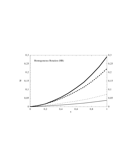
Figure 1: $\mu$ vs $\tau$ for $n=4$; HR₁,$r_{a}=1.5$ (thin solid line); HR₁, $r_{a}=100$ (thin dashed line) and HR₂,$r_{a}=1.5$ (bold Solid line); HR₂, $r_{\rm a}=100$ (bold dashed line)

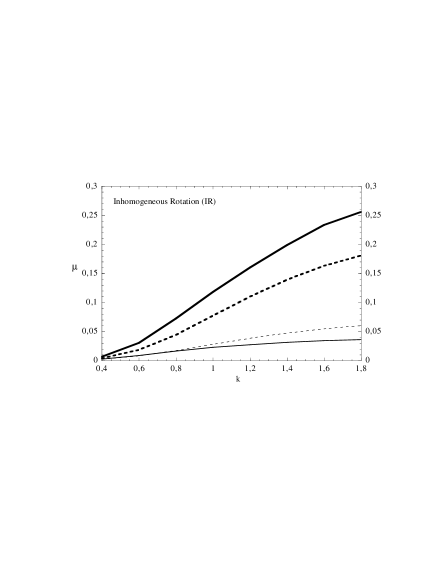
Figure 2: $\mu$ vs $k$ for $n=4$, IR₁, $r_{\rm a}=1.5$ (thin solid line); IR₁, $r_{\rm a}=100$ (thin dashed line) and IR₂, $r_{\rm a}=1.5$ (bold Solid line); IR₂, $r_{\rm a}=100$ (bold dashed line)

4 Influence of the Rotation on the Stability

Using the N-body code described in Alimi and Scholl (1993), we have performed on Connection-Machine 5 a series of numerical simulations of the evolution of the systems defined in the previous section. As the collisionless hypothesis is fundamental for interpreting our results, we have not continued our simulations beyond a few hundred dynamical times in order to avoid the later evolution where two-body relaxation arises. However, all our models reach a steady state before about $50~{}T_{d}$ (where the initial dynamical time is estimated by the following formula $T_{d}=\sqrt{\sum r^{2}_{i}/\sum v^{2}_{i}}$, the summations on initial positions and velocities are done on all the particles). We will then present our results for this interval.

The physical mechanism of the radial-orbit instability for collisionless self-gravitating systems is well known. It has been described in detail by several authors (see [Palmer 1994] for example). The morphological deformation of the initial gravitational system resulting from this instability is mainly due to the trapping of particles with a low angular momentum in a bounded area of space. This trapping favors a deformation of the initial spherical system to an ellipsoidal or even a bar-like structure. To evaluate such a deformation, it is convenient to use the axial ratio defined from the moment of inertia tensor $I$ [Allen et al. 1990]. From the three real eigenvalues of $I$, $\lambda_{1}\geq\lambda_{2}\geq\lambda_{3}$, we compute the axial ratios $a_{1}=\lambda_{2}/\lambda_{1}$ and $a_{2}=\lambda_{2}/\lambda_{3}$. These two quantities, which can always be defined because these eigenvalues never vanish, satisfy $a_{1}\leq 1\leq a_{2}$. In order to discriminate clearly between a bar-like structure, a quasi-sphere and a disk-like structure , we define the quantity $f$ from $a_{1}$ and $a_{2}$

$$f=\frac{1-a_{1}}{a_{2}-1}$$ (10)

A bar-like structure is characterized by $a_{1}<1$ and $a_{2}\simeq 1$ which implies a $f$ value significantly larger than $1$. A disc-like structure is characterized by $a_{1}\simeq 1$, $a_{2}>1$ and $0<f<1$. Any system with a $f$ value of order unity has a quasi-spherical structure.

4.1 Rotating systems according to Method 1

This type of rotation preserves the anisotropy of the non-rotating OM systems. The distribution function of the rotating system depends only on the variable $Q\;=\;E+L^{2}/2r_{\rm a}^{2}$ as in the case of the non-rotating systems. We see in Table 1 that, in the case $n=4$, the stability parameters defined in Section 2.2 are very weakly modified whatever the $\tau$ and $k$ parameters values are, that is to say, whatever the rotational kinetic energy is (low with this method). According to the conditions given by equations 5 and 6, we expect the (in)stability of the original non-rotating systems not to be modified when they are put in rotation. Our numerical simulations confirm this. In figure 3, we see that the evolution of axial ratios is similar for the rotating (dashed and dotted lines) and non-rotating (solid lines) systems. This results holds for the homogeneous and inhomogeneous rotations and whatever the $n$ parameter value is.

HR1					IR1
	$r_{\rm a}=1.5$		$r_{\rm a}=100$			$r_{\rm a}=1.5$		$r_{\rm a}=100$
$\tau$	$P_{\varepsilon}$	$P_{\lambda}$	$P_{\varepsilon}$	$P_{\lambda}$	$k$	$P_{\varepsilon}$	$P_{\lambda}$	$P_{\varepsilon}$	$P_{\lambda}$
0.0	22.42	1.39	13.84	4.07	0.4	24.54	1.31	15.25	3.89
0.2	22.83	1.41	14.28	4.12	0.6	24.04	1.31	14.60	3.84
0.4	22.76	1.39	14.05	4.23	0.8	24.02	1.33	14.44	3.75
0.6	22.22	1.41	13.68	4.22	1.0	23.57	1.27	17.18	3.77
0.8	22.04	1.42	13.34	4.08	1.2	22.04	1.25	14.09	3.79
1.0	21.93	1.44	12.98	4.18	1.4	23.59	1.26	13.99	3.79

Table 1: Stability parameter evolution for the first method for rotating systems with $n=4$

Figure 3: The axial ratio vs. dynamical time for $n=4$; $r_{\rm a}=100$-HR₁ (top-left panel), $r_{\rm a}=100$-IR₁ (top-right panel), $r_{\rm a}=1.5$-HR₁ (bottom-left panel) and $r_{\rm a}=1.5$-IR₁ (bottom-right panel). The amount of rotation is represented by using different kinds of lines. Solid lines: $\tau=0$(HR) or $k=0$ (IR), dotted lines : $\tau=0.3$ (HR) or $k=0.6$ (IR) and dashed lines : $\tau=0.8$ (HR) or $k=1.4$ (IR).

4.2 Rotating systems according to the second method

The situation is now more complicated because the rotation procedure modifies the system’s anisotropy. In the second method, the stationary OM distribution function is modified by a positive definite and time-independant transformation. The resulting DF is then always stationary and positive definite. Moreover as the modified systems are always spherical (no modification on positions have been performed), the new DF depends only on isolating integrals of motion, the energy and the squared angular momentum [Perez & Aly 1996]. It is therefore a stationary solution of the collisionless Boltzmann-Poisson system. We have also verified that the resulting systems are always virialized, as confirmed by figure 4.

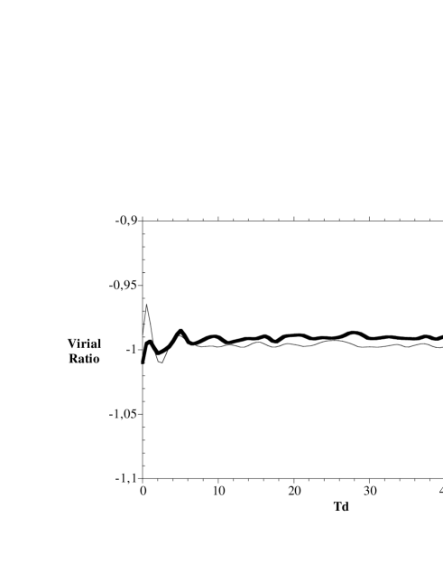
Figure 4: The evolution of the Virial ratio for the initial systems defined respectively by $n=4$, $r_{a}=1.5$, and $n=4$, $r_{a}=100$ which have acquired their rotation according to the procedure HR₂ with $\tau=30\%$ (thin line) and IR₂ with $k=1.4$ (bold line) . A similar evolution for the Virial ratio (remaining very close to 1) is obtained for all runs.

Let us first consider rotating systems with high values of $r_{\rm a}$. We recall that non-rotating OM systems with the same anisotropy parameter are stable [Perez et al. 1996]. The dynamical evolution obtained for such systems in our present simulations (see Figure 5, top panels) allows us to distinguish two classes of behavior. When $r_{\rm a}$ is large and the rate of rotation stays modest (typically $\mu<10\%$), we find that systems remain stable and spherical ($a_{1}\simeq a_{2}$, $f\simeq 1$). However, when $r_{\rm a}$ is large and the rate of rotation becomes important (typically $\mu>10\%$), we find that initially spherical systems develop a very soft bar-like instability ($a_{2}\simeq 1$, $a_{1}\simeq 0.85$, $f\simeq 1.3$).

Systems with small $r_{\rm a}$ values have instead a different behavior, which depends on whether the rotational motion has been introduced by using a homogeneous or an inhomogeneous procedure. In the first case (HR₂ procedure), Figure 5 (bottom-left panel) shows that systems which are radial orbit-unstable without rotation (e.g., $a_{1}\simeq 0.55,a_{2}\simeq 1$, $f\gg 1$) (solid line), become quasi-spheroidal ($a_{1}\simeq 0.85$, $a_{2}\simeq 1.1$, $f\simeq 1.3$) when they have a modest rotation motion ($\mu<10\%$) (dotted line). However, when rotation is important (typically $\mu>10\%$), such systems develop a disc-like instability ($a_{1}\simeq 1$, $a_{2}\simeq 1.25$, $f\simeq 0$) (dashed line). In the second case (IR₂ procedure)(bottom-right panel), the fact that rotation has been introduced only in a central region of the system prevents one from obtaining quasi-spherical systems and, therefore, the radial-orbit instability persists ($a_{1}\simeq 0.65$, $a_{2}\simeq 1.1$, $f\simeq 3.5$) for systems with a modest amount of rotation ($n=4$;IR₂;$r_{\rm a}=1.5$;$k=0.6$) (dotted line). When the amount of rotation is high enough ($\mu>10\%$) a disc-like structure appears ($a_{1}\simeq 1$, $a_{2}\simeq 1.25$, $f\simeq 0$), as in the HR₂ procedure. The evolution of the axial ratio for the system ($n=4$; IR₂; $r_{a}=1.5$; $k=1.4$) is represented by dashed line. These results hold whatever the $n$ parameter value is. In practice we have performed numerical simulations for three values of $n$ ($n=3.5,4,4.5$).

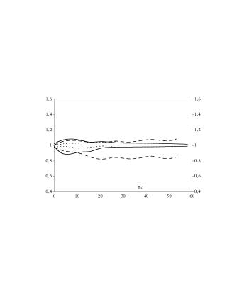
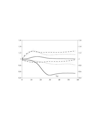
Figure 5: The axial ratios vs. dynamical time for $n=4$; $r_{a}=100$-HR₂ (top-left panel), $r_{a}=100$-IR₂ (top-right panel), $r_{a}=1.5$-HR₂ (bottom-left panel) and $r_{a}=1.5$-IR₂ (bottom-right panel). The amount of rotation is represented by using different kinds of lines: solid lines : $\tau=0$(HR) or $k=0$ (IR), dotted lines: $\tau=0.3$(HR) or $k=0.6$ (IR), and dashed lines: $\tau=0.8$(HR) or $k=1.4$ (IR).

Are the stability parameters $P_{\epsilon}$ and $P_{\lambda}$ still discriminating for such rotating systems?. We can see in Table 2 that non-rotating stable systems ($r_{\rm a}=100$) are predicted to remain stable when the second rotation method is applied ($P_{\epsilon}$ stays smaller than 20 and $P_{\lambda}$ stays larger than 2.5) whatever the $\tau$ and $k$ parameters values are. On the other hand, non-rotating radial-orbit unstable systems ($r_{\rm a}=1.5$) are predicted to become stable when sufficient Method 2 rotation is applied, from $\tau=0.4$ and $k=0.8$ which correspond on figures 1 and 2 to typically $\mu\simeq 5\%$. As a matter of fact, in this case, $P_{\epsilon}$ becomes less than 20 and $P_{\lambda}$ becomes greater than 2.5. Consequently, these stability parameters which have been constructed to predict the stability of non-rotating spherical systems are not relevant as soon as the quantity of kinetic rotation energy becomes large, typically $\mu\ga 10\%$.

HR₂ IR₂ $r_{\rm a}=100$ $r_{\rm a}=1.5$ $r_{\rm a}=100$ $\tau$ $P_{\varepsilon}$ $P_{\lambda}$ $P_{\varepsilon}$ $P_{\lambda}$ k $P_{\varepsilon}$ $P_{\lambda}$ $P_{\varepsilon}$ $P_{\lambda}$ 0.0 22.42 1.39 13.84 4.07 0.4 23.50 1.81 17.93 3.51 0.2 21.31 1.94 13.43 4.08 0.6 21.68 2.17 13.34 3.57 0.4 19.21 2.92 12.32 4.10 0.8 18.43 2.81 11.67 3.67 0.6 16.96 3.55 10.46 4.17 1.0 16.56 3.17 10.55 3.75 0.8 14.08 4.04 8.97 4.22 1.2 15.23 3.62 9.39 3.80 1.0 11.24 4.58 7.40 4.46 1.4 13.85 3.97 8.64 3.96

Table 2: Evolution of the stability parameter for systems with $n=4$ and put in rotation by using the second method

5 Physical Interpretation and Conclusions

The rotational properties of collapsed systems depend to a large extent on the amount of angular moment before the collapse. In order to study in a realistic way the importance of rotation for the dynamics of self-gravitating systems, it is necessary either to attempt an analytical approach, or to perform a complete numerical study modelling the collapse and relaxation phases prior to the two-body relaxation phase. However, although the collapse of a system can be studied by using the introduced amount of rotational kinetic energy as parameter, it is difficult to extract general conclusions from this kind of experiments. As a matter of fact in this way the post-collapse physical features of the object cannot be completely controlled and hence it can then be difficult to study with these methods the influence of the rotation on post-collapse systems.

This justifies the method that we have used in this paper. Starting from virialized systems with exactly known dynamical properties, we can study the influence of rotation by controlling its features. If the initial systems cover a wide variety of physical properties, and if the methods to introduce the rotation preserve certain fundamental features of these systems (invariance of mean energy, conservation or controlled modification of the distribution function), the numerical study will then be able to be used as a model to extract some general conclusions. As a matter of fact, our simulations start from a wide variety of initial conditions fully controllable through the dependence on the two parameters $n$ and $r_{a}$. On the other hand, the techniques used to introduce rotation to the systems preserve (as explained in Section 3) the properties that ensure that our models are spherical stationary solutions of the collisionless Boltzmann-Poisson system.

The main properties found in our study are the following :

• There do not exist spherical self-gravitating systems in ”fast” rotation. Our simulations show in fact that, when $\mu\ga 10\%$, the systems do not remain spherical but become lengthened along one or two axes depending on whether they are isotropic or anisotropic, respectively, when they do not have a rotational motion.

• Rotation (in our case HR₂ and IR₂) can allow for a reorganization of systems in velocity space able to modify their dynamical behavior. We have in fact shown that a moderate rotation (typically $0\leq\mu\la 10\%$) can stabilize and confer a quasi-spherical structure to systems that, when they are not rotating, suffer a radial-orbit instability. Therefore, there can exist rotating spherical self-gravitating systems. This is the case for our models with $r_{\rm a}\ga 2$ and $\mu\la 10\%$.

• We have finally found that the stability parameters introduced in [Perez et al. 1996] remain valid as long as $\mu\la 10\%$.

6 Appendix: Generation of initial conditions

6.1 The initial positions for the particles

Let us consider a density $\rho_{iso}$ given by the polytropic relation $\rho_{iso}=c_{n}\psi_{iso}^{n}$, where

$$c_{n}=\frac{(2\pi)^{n}\Gamma(n-1/2)}{\Gamma(n+1)}\;\;\;\;,\;\;\Gamma(n+1):=\int_{0}^{\infty}\!\!x^{n}e^{-x}dx$$

and $\psi_{iso}$ is the solution of the Lame-Emden equation

$$\frac{1}{r^{2}}\frac{d}{dr}\left(r^{2}\frac{d\psi}{dr}\right)+4\pi Gc_{n}\psi^{n}=0$$

This isotropic model is then deformed according to

$$\rho_{ani}(r)=(1+\frac{r^{2}}{r_{a}^{2}})\rho_{iso}$$

where the anisotropic radius $r_{a}$ is a parameter which controls the deformation. The polytropic index $n$ is chosen in the range $]0.5,5]$ in order to the system admits a finite mass $M(<r)=4\pi\int_{0}^{r}r^{2}\rho_{ani}(r)dr$. The total mass of the system is normalized to unity and we then compute for a large set of particles ($1\leq i\leq N$) from the inverse function of $M(x)$ and $sin(x)$, the components

$$r_{i}=r_{max}M^{-1}(x)$$

$$\theta_{i}=2\arcsin(\sqrt{x})$$

$$\phi_{i}=2\pi.x$$

where $x$ is an uniform random variable on $[0,1]$. The size of the system $r_{max}$ is chosen such that $\rho_{ani}(r>r_{max})<10^{-5}$.

6.2 The initial velocities for particles

Let us consider the velocity components in spherical coordinates ($v_{r},v_{\theta},v_{\phi}$), we compute $v_{t}=\sqrt{v_{\theta}^{2}+v_{\phi}^{2}}$ and $\alpha\;=\;\arctan(v_{\theta}/v_{\phi})$. The probability $p(\Gamma)$for finding a particle in a volume $d\Gamma:=dr\;d\theta\;d\phi\;dv_{r}\;dv_{\theta}\;d\alpha$ of the phase space is defined from the DF of the system

$$p(\Gamma)d\Gamma=\frac{1}{N}f(\Gamma)r^{2}dr\sin\theta d\theta d\phi v_{t}dv_{t}dv_{r}d\alpha$$ (11)

In the Ossipkov-Merritt model DF is a function only on $Q$ variable

$$f=f(Q)\;\;\;\mbox{with}\;\;\;Q=\frac{1}{2}v_{r}^{2}+\frac{1}{2}\left(1+\frac{r^{2}}{r_{a}^{2}}\right)v_{t}^{2}+\psi(r)$$ (12)

the equation (11) then reduces to

$$\int p(\Gamma)d\Gamma=\int\frac{8\pi^{2}r^{2}v_{t}}{N}f(r,v_{r},v_{t})dr\;dv_{t}\;dv_{r}$$ (13)

$r$, $v_{r}$ and $v_{t}$ are dependant random variables. In order to continue the integration of equation (13) we introduce the variables $R$ and $\beta$ defined as following

$$v_{r} = R.\cos\beta$$

$$v_{t}\sqrt{1+\displaystyle{\frac{r^{2}}{r_{a}^{2}}}} = R.\sin\beta$$

We then get

$$f(r,v_{r},v_{t})\frac{8\pi r^{2}v_{t}}{N}=f\left(\frac{R^{2}}{2}+\psi(r)\right)\frac{8\pi^{2}r^{2}R^{2}\sin\beta}{N\left(1+\displaystyle{\frac{r^{2}}{r_{a}^{2}}}\right)}drdRd\beta$$

We see from the previous expression that the random variable $\beta$ is $r$ and $R$ independant and we have

$$p(\beta)d\beta = \frac{\sin\beta}{2}d\beta$$

$$p(r,R)drdR = \frac{16\pi^{2}r^{2}R^{2}}{1+\displaystyle{\frac{r^{2}}{r_{a}^{2}}}}f\left(\frac{R^{2}}{2}+\psi(r)\right)drdR$$

The conditional probablity for finding a particle with a velocity defined by $R$ at a given distance $r_{0}$ is then

$$p(R\mid r_{0})=\frac{p(r_{0},R)}{p(r_{0})}\;\;\;\;\;\mbox{with}\;\;\;\;\;p(r_{0})=\frac{4\pi r^{2}\rho(r_{0})}{M(=1)}$$ (14)

and finally

$$P(R\mid r=r_{o}) = \frac{4\pi}{\rho(r_{o})\left(1+\frac{r_{o}^{2}}{r_{a}^{2}}\right)}\int_{0}^{R}R^{\prime 2}f(\frac{R^{\prime 2}}{2}+\psi(r_{o}))dR^{\prime}$$ (15)

$$= \frac{2\pi}{\rho(r_{o})\left(1+\frac{r_{o}^{2}}{r_{a}^{2}}\right)}\int_{\psi(r_{o})}^{\psi(r_{o})+\frac{R^{2}}{2}}\!\!\frac{f(Q)dQ}{\sqrt{2(Q-\psi(r_{o}))}}$$

We are now able to assign a velocity for each particle which the position have been previously determined.

$$R_{i} = P^{-1}(x|r=r_{o})$$

$$\beta_{i} = 2\sin^{-1}(\sqrt{x})$$

$$\alpha_{i} = 2\pi.x$$

where $x$ is an uniform random variable on $[0,1]$, and $P^{-1}$ is the inverse function of the probability defined by equation (15). Finally

$$v_{r\;i} = R_{i}.cos\beta_{i}$$

$$v_{\theta\;i} = \sqrt{1+\frac{r_{o}^{2}}{r_{a}^{2}}}.R_{i}.\sin\beta_{i}\cos\alpha_{i}$$

$$v_{\phi\;i} = \sqrt{1+\frac{r_{o}^{2}}{r_{a}^{2}}}.R_{i}.\sin\beta_{i}\sin\alpha_{i}$$

References

- [Allen et al. 1990] Allen A.J., Palmer P.L., Papaloizou J., 1990, MNRAS, 242, 576
- [Alimi & Scholl 1993] Alimi J. M., Scholl H., 1993, Int. J. Mod. Phys. C., 4, 197
- [Antonov 1973] Antonov, V.A., On the instability of stationary spherical models with purely radial motion in The dynamics of galaxies and star clusters, Ed: Omarov, G.B., Alma Ata: Nauka 1973 (in russian), in Structure and Dynamics of Elliptical Galaxies, IAU Symp 127, Ed: de Zeeuw, T., Dordrecht, Reidel 1987 (in english).
- [Barnes et al. 1986] Barnes J., Goodman J., Hut, P., 1986, ApJ, 300, 112
- [Binney & Tremaine 1987] Binney J., Tremaine S., 1984, Galactic Dynamics, Princeton University Press
- [IAU Colloquium 157] Ed. Buta, R., Crocker, D.A., Elmegreen, B.G., 1996, IAU Colloquium 157, Barred Galaxies, Astronomical Society of the Pacific Conference Series, vol 191.
- [Calot 1973] Calot G., 1973, Cours de Statistiques Descriptives, Dunod, Paris
- [einsel971997] Einsel, C., Spurzem, R., 1997, submitted to MNRAS, Sissa astro-ph9704284.
- [Goodwin 1997] Goodwin S.P., 1997, MNRAS, 286, 139
- [Lynden-Bell1962] Lynden-Bell D, 1962, MNRAS, 124,1
- [Merritt 1985a] Merritt D., 1985a, AJ, 86, 1027
- [Merritt 1985b] Merritt D., 1985b, MNRAS, 214, 25P
- [Navarro & White 1993] Navarro, J.E., White, S.D.M. 1993, MNRAS, 265, 271
- [Ossipkov 1979] Ossipkov, L.P., Pis’ma Astron. Zh., 5, 77
- [Palmer & Papaloizou 1986] Palmer P.L., Papaloizou J., 1986, MNRAS, 224, 1043
- [Palmer 1994] Palmer P.L., 1994, Stability of Collisionless Stellar Systems, Kluwer Academic Publishers, Dordrecht
- [Papaloizou et al. 1991] Papaloizou,J., Palmer P.L., Allen A.J., 1991, MNRAS, 253, 129
- [Perez & Aly 1996] Perez J., Aly J.J., 1996, MNRAS, 280, 689
- [Perez et al. 1996] Perez J., Alimi, J.-M., Aly J.-J., Scholl, H., 1996, MNRAS, 280, 700
- [Staneva et al. 1996] Stavena A., Spassova, N., Golev, V. 1996, A&AS 116, 447
- [de Zeeuw & Franx 1991] de Zeeuw P.T., Franx M., 1991, ARAA, 29, 239