HIRES Spectroscopy of APM 08279+5525: Metal Abundances in the Ly$\alpha$ Forest

Abstract

We present high S/N echelle spectra of the recently discovered ultraluminous QSO APM 08279+5255 and use these data to re-examine the abundance of Carbon in Ly$\alpha$ forest clouds. In agreement with previous work, we find that approximately 50% of Ly$\alpha$ clouds with hydrogen column densities log $N$(H I)$\geq 14.5$ have associated weak C IV absorption with log $N$(C IV)$\lower 2.15277pt\hbox{$\;\buildrel>\over{\sim}\;$}12$, and derive a median $N$(C IV)/$N$(H I)$=1.4\times 10^{-3}$. The agreement with earlier estimates of this ratio may be somewhat fortuitous, however, because we show that previous analyses have probably overestimated the number of Ly$\alpha$ clouds which should be included in this statistic.

We then investigate whether there is any C IV absorption associated with weaker H I column densities by stacking 51 C IV regions corresponding to 51 Ly$\alpha$ lines with $13.5\leq{\rm log}N{\rm(H~{}I)}\leq 14.0$. The co-added spectrum has S/N $\simeq 580$ but shows no composite C IV absorption. In order to understand the significance of this non-detection we have stacked together 51 theoretical C IV $\lambda 1548$ lines with individual values of column density and velocity dispersion scaled appropriately from the values measured in the corresponding Ly$\alpha$ lines. We find that even if the typical value $N$(C IV)/$N$(H I)$=1.4\times 10^{-3}$ applies to these lower column density clouds, the corresponding signal in the stacked C IV region is smeared by the likely random difference in redshift between C IV and Ly$\alpha$ absorption and becomes very difficult to recognize. This seems to be a fundamental limitation of the stacking method which may well explain why in the past it has led to underestimates of the metallicity of the Ly$\alpha$ forest.

We also analyze our spectra with the pixel-by-pixel optical depth technique recently developed by Cowie & Songaila (1998) and find evidence for net C IV absorption in Ly$\alpha$ clouds with optical depths as low as $\tau{\rm(Ly\alpha)}=0.5-2$, as these authors did. However, we show with simulations that even this method requires higher sensitivities than reached up to now to be confident that the ratio $N$(C IV)/$N$(H I) remains constant down to column densities below log $N$(H I)$\simeq 14.0$ . We conclude that the question of whether there is a uniform degree of metal enrichment in the Ly$\alpha$ forest at all column densities has yet to be fully answered. Future progress in this area will probably require concerted efforts to push further the detection limit for C IV lines in selected bright QSOs.

1 Introduction

Nearly thirty years after its discovery by Lynds (1971), the Ly$\alpha$ forest continues to provide fertile ground for observational and theoretical studies. New echelle spectrographs on large telescopes, most notably the High Resolution Spectrograph (HIRES, Vogt et al. (1994)) on Keck I, have provided spectra of exceptional quality and detail. This has permitted extensive study of many important properties of the Ly$\alpha$ forest as comprehensively reviewed by Rauch (1998). Complementary to this quality observational data, cosmological simulations which utilize gas hydrodynamics have improved our understanding of the nature of the forest clouds. These simulations have shown that the formation of the Ly$\alpha$ forest is a natural consequence of the growth of structure in the universe through hierarchical clustering in the presence of a UV ionizing background (e.g. Cen et al. (1994); Petitjean, Mucket & Kates (1995); Hernquist et al. (1996); Bi & Davidsen (1997)). In this class of models, low column density H I clouds (log $N$(H I)$<$14, where $N$(H I) is measured in cm^-2) are found preferentially in voids whilst stronger lines are associated with higher density clouds which arise in filamentary structures around collapsed objects.

Important clues to the origin of Ly$\alpha$ clouds can be gleaned from their clustering properties and chemical composition. Early investigations of the Ly$\alpha$ forest found no evidence of metals associated with the H I clouds, suggesting that they consisted of pristine material (Sargent et al. (1980)). More concerted efforts however, did provide some evidence for metals in the forest either individually (Meyer & York 1987) or in a stacked spectrum (Lu 1991). The realization that metal enrichment is in fact widespread in high column density Ly$\alpha$ clouds has come relatively recently with the availability of HIRES on the Keck I telescope. A number of studies (e.g. Tytler et al. (1995); Cowie et al. (1995); Songaila & Cowie (1996)) have found that C IV absorption is seen in approximately 50% of forest clouds with log $N$(H I)$>$14.5 and in about 90% of clouds with log $N$(H I)$>$15. Evidently the intergalactic medium (IGM) has been enriched by the products of stellar nucleosynthesis even at redshifts as high as $z\sim 3.5$. Photoionization models (e.g. Hellsten et al. (1997)) can reproduce the observed C IV/H I ratio at $z\sim 3$ for a typical Carbon abundance [C/H] = $-2.5$ . Rauch, Haehnelt, & Steinmetz (1997) predict an order of magnitude scatter in [C/H] in models where random sight-lines are cast through protogalactic clumps, a prediction corroborated by the data.

Two scenarios have been suggested to explain the presence of metals in the Ly$\alpha$ forest; early pre-enrichment by a widespread episode of star formation, possibly associated with Pop III stars, or in-situ enrichment whereby the H I cloud is enriched locally either by contamination from a nearby galaxy or by star formation within the cloud itself (Ostriker & Gnedin (1996); Gnedin & Ostriker (1997)). Cosmological simulations of a two phase ISM recently performed by Gnedin (1998) confirm the results of Gnedin & Ostriker (1997) that the dominant process for transportation of heavy elements into the IGM is mergers of protogalaxies in dark matter halos. One may expect that for the scenario of in-situ enrichment, where metals are synthesized relatively close to the Ly$\alpha$ clouds being observed, the metallicities would be highly inhomogeneous depending on the proximity of a given Ly$\alpha$ cloud to a star-forming region and its past merger history. If, however, the bulk of the metals is formed by an episode of Pop III star formation at sufficiently high redshift ($z\sim 14$ in the models of Ostriker & Gnedin 1996), a more uniform [C/H] may have been established by $z\sim 3$, if the mixing mechanism is efficient.

Discrimination between these two enrichment scenarios is probably best addressed in the low column density regime. Since the optical depth of Ly$\alpha$ clouds is roughly indicative of the baryon overdensity, studying low column density lines will give us an insight into the low mass systems. In the simulations of Gnedin & Ostriker (1997), for example, a sudden drop in metallicity is predicted for Ly$\alpha$ clouds with log $N$(H I)$<$14 where the star formation rate is expected to be much lower than in higher density clouds. However, determining the [C/H] abundance in weak Ly$\alpha$ clouds has been observationally challenging due to the extreme weakness of C IV absorption when log N(H I) $\lower 2.15277pt\hbox{$\;\buildrel<\over{\sim}\;$}14$. In order to overcome the difficulty of a direct C IV detection, this problem has recently been tackled with two different approaches which have produced apparently conflicting results.

Lu et al. (1998) tackled the problem by stacking almost 300 C IV regions to produce a composite spectrum, a method first applied to QSO spectra by Norris, Peterson & Hartwick (1983). Having found no C IV in their summed spectrum (which had a final S/N ratio of 1860) Lu et al. used Monte Carlo simulations to place an upper limit on the Carbon abundance in clouds with log $N$(H I)$<14$ of [C/H]$<-3.5$. A different conclusion was reached by Cowie & Songaila (1998) who used distributions of Ly$\alpha$ optical depths, $\tau{\rm(Ly\alpha)}$, to build distributions of corresponding $\tau$(C IV) on a pixel-by-pixel basis. A comparison between the $\tau$(C IV) distribution and a reference ‘blank’ distribution showed a residual signal sufficiently strong to be consistent with [C/H]$\simeq-2.5$ for Ly$\alpha$ clouds with log $N$(H I) as low as 13.5. Thus, whilst Lu et al. interpreted their results as evidence against a uniform enrichment of the IGM at $z\sim 3$, Cowie & Songaila proposed that transportation/ejection mechanisms from early sites of star formation are much more efficient than anticipated, in order to pollute Ly$\alpha$ clouds uniformly over a range of N(H I) of nearly 4 orders of magnitude.

In this paper we aim to address the contradiction between these two earlier analyses by taking another look at the metallicity in the Ly$\alpha$ forest using new data which are among the best ever obtained for this purpose; almost 9 hours of HIRES observations (described in §2) of the ultra-luminous QSO APM 08279+5255. In §3 we define the redshift interval over which we search for C IV absorption; the very high S/N of the spectrum in the C IV region allows us to refine earlier estimates of the typical C IV/H I ratio in Ly$\alpha$ lines with log $N$(H I)$>14.5$ (§4). In §5 we investigate whether this high quality, independent data set can help resolve the current discrepancy between the results of Lu et al. (1998) and Cowie & Songaila (1998), thus shedding some light on the origin of the metals observed in low column density Ly$\alpha$ clouds. We summarize our main results in §6.

2 Observations and Data Reduction

The target for these observations is APM 08279+5255, an ultra-luminous Broad Absorption Line (BAL) quasar discovered by Irwin et al. (1998) during a survey of Galactic halo carbon stars. The emission redshift $z_{\rm em}=3.87$ measured by Irwin et al. from the C IV $\lambda 1549$ and N V $\lambda 1240$ emission lines has recently been refined to $z_{\rm em}=3.9110$ by Downes et al. (1999) who detected CO emission. Given the difficulty in measuring a precise redshift from the UV emission lines which are affected by the BAL phemomenon, the difference is probably not significant; in the following analysis we adopt $z=3.9110$ as the systemic redshift of the QSO. Positionally coincident with an IRAS Faint Source Catalog object with a 60 micron flux of 0.51Jy, APM 08279+5255 has an optical R magnitude=15.2 and an inferred bolometric luminosity of $5\times 10^{15}$L_⊙ making it the most luminous object currently known. Adaptive optics imaging with the CFHT (Ledoux et al. (1998)) has resolved APM 08279+5255 into two images separated by 0.35 arcsec in the NE–SW direction with an intensity ratio $I_{NE}$/$I_{SW}=1.2\pm 0.25$ in the $H$-band.

For our purposes, APM 08279+5255 is a nearly ideal background source for investigating the Ly$\alpha$ forest and associated metal absorption lines at high S/N ratio and resolution. The data presented here were obtained with HIRES on the Keck I telescope on three runs in April and May 1998. Details of the observations are presented in Table 1. APM 08279+5255 is unresolved in these observations. The cross disperser and echelle angles were used in a variety of settings to give almost complete wavelength coverage between 4400 and 9250 Å. The emission spectrum of a Th-Ar hollow cathode lamp provided a wavelength reference and a continuum source internal to the spectrograph was used for a first order correction of the echelle blaze function.

The data were reduced using Barlow’s (1999, in preparation) customized HIRES reduction package (HAR). The individual, sky-subtracted spectra were mapped onto a linear wavelength scale with a dispersion of 0.04 Å per wavelength bin and then co-added with a weight proportional to their S/N. Finally, this co-added spectrum was normalized by fitting a cubic spline function with STARLINK software to continuum regions deemed to be free of absorption. Even in the dense forest of Ly$\alpha$ lines at wavelengths below that of Ly$\alpha$ emission, continuum windows can be identified at the high resolution of our data.

The final co-added spectrum has a resolution of 6 km s^-1, sampled with $\sim$ 3.5 wavelength bins, and S/N between 30 and 150. Over the range of interest for C IV absorption (see §3 below) the typical signal-to-noise ratio is S/N $\simeq 80$. At the mean $z_{\rm abs}=3.41$ the $5\sigma$ detection limit for the rest-frame equivalent width of C IV absorption line with the typical FWHM = 22 km s^-1 (see later) is $W_{0}$(1548)$=3$ mÅ, which corresponds to a column density log $N$(C IV) = 11.88 . Thus these data are comparable to those obtained by Songaila & Cowie (1996) for Q0014+813 and Q1422+231, their best observed QSOs.

The full spectrum is described elsewhere (Ellison et al. 1999) and is available via anonymous ftp from ftp.ast.cam.ac.uk (pub/sara/APM0827).

3 Sample Definition

APM 08279+5255 belongs to a class of objects whose spectra are known to exhibit broad, high velocity, intrinsic absorption lines. Before proceeding we must therefore define a working wavelength interval over which we can study C IV and Ly$\alpha$ lines in our spectrum and be confident that we are not confusing them with absorption from ejected material. The upper limit of this interval (for C IV) is 7280 Å  ($z_{\rm max}=3.701$), at the blue edge of the broad C IV absorption trough which corresponds to an ejection velocity $v_{\rm ej}\simeq 13100$ km s^-1 relative to the systemic redshift. The lower limit for the C IV interval is 6365 Å ($z_{\rm min}=3.109$), the wavelength of Ly$\beta$ emission. We excluded the region of the spectrum blueward of this wavelength in order to avoid confusion of Ly$\alpha$ with Ly$\beta$ lines. We further excluded a small region between 6860 and 6950 Å which is contaminated by the atmospheric B band.

In principle, some of the C IV doublets in our sample could still be related to the BAL phenomenon and be intrinsic to the QSO rather than intervening absorbers, since ejecta have been observed at velocities as large as 60,000 km s^-1. However, we found no evidence of this in APM 08279+5255. For example, none of the C IV systems at $z_{\rm abs}<z_{\rm max}$ show any indication of partial coverage of the QSO (one of the signatures of intrinsic absorption), whereas we do see such an effect for systems at $z_{\rm abs}>z_{\rm max}$. Most importantly, as we will discuss below, the density of C IV absorbers per unit redshift between $z_{\rm min}$ and $z_{\rm max}$ is entirely compatible with that measured towards non-BAL QSOs—there is no excess of C IV absorbers within our working wavelength interval.

4 C IV In Ly$\alpha$ Clouds with log $N$(H I) $\geq 14.5$

Before addressing the question of CIV absorption in Ly$\alpha$ clouds with 13.5$\leq$ log N(H I) $\leq 14.0$, the first stage of our analysis is to determine the typical $N$(C IV)/$N$(H I) ratio in Ly$\alpha$ clouds with log $N$(H I) $\geq 14.5$. The aim is to provide an independent measure of this quantity, and therefore of the metallicity of Ly$\alpha$ clouds, for comparison with the results of Cowie et al. (1995) and Songaila & Cowie (1996).

These authors found that at a detection limit log $N$(C IV) $\geq 12.0$ approximately half of the Ly$\alpha$ lines with log $N$(H I)$\geq 14.5$ have associated C IV absorption. Ly$\alpha$ lines above this column density cut-off are saturated and therefore not on the linear part of the curve of growth. Therefore, an accurate $N$(H I) cannot normally be measured without higher-order Lyman lines such as Ly$\beta$ or Ly$\gamma$ that are not saturated. Cowie et al. (1995) circumvented this difficulty by assuming that at log $N$(H I)$\geq 14.5$ the residual flux in the core of a Ly$\alpha$ absorption line is $r_{f}<0.025$ for the mean value of the Doppler parameter of $b=34$ km s^-1 determined by Carswell et al. (1991). This approach is of course critically sensitive to a precise determination of the zero level.

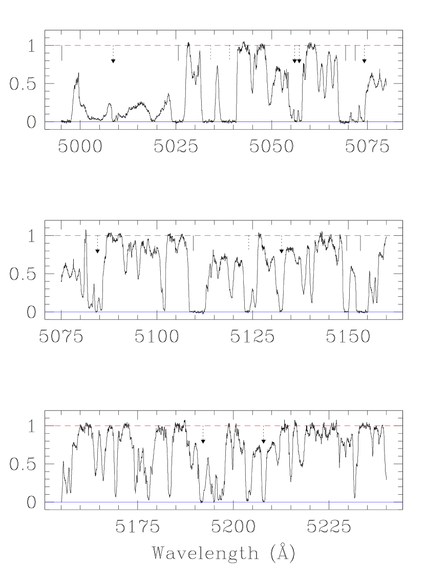
Figure 1: The Ly$\alpha$ forest in APM 08279+5255 within the redshift range $z=3.109-3.701$ of our analysis. The $y$-axis is normalized counts. Vertical tick marks near the continuum level indicate Ly$\alpha$ lines with residual flux $r_{f}<0.025$; solid and broken tick marks are used to indicate lines with and without associated C IV $\lambda\lambda 1548,1550$ absorption, respectively. Solid triangles flag Ly$\alpha$ lines with column density log $N$(H I)$<14.5$ even though $r_{f}<0.025$ (see text). The horizontal black line between 5387 and 5456 Å indicates the region of the forest omitted from the analysis because the corresponding C IV wavelengths fall within the atmospheric B band.

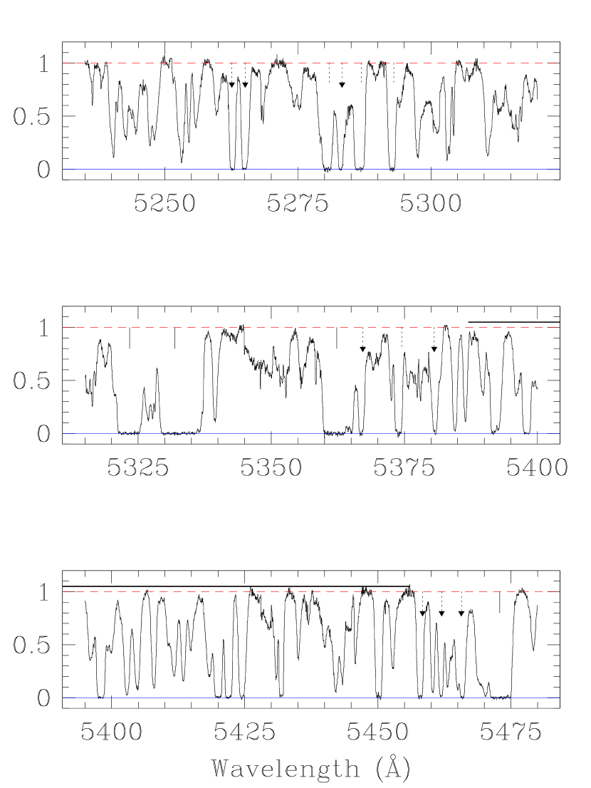
Figure 1: Continued

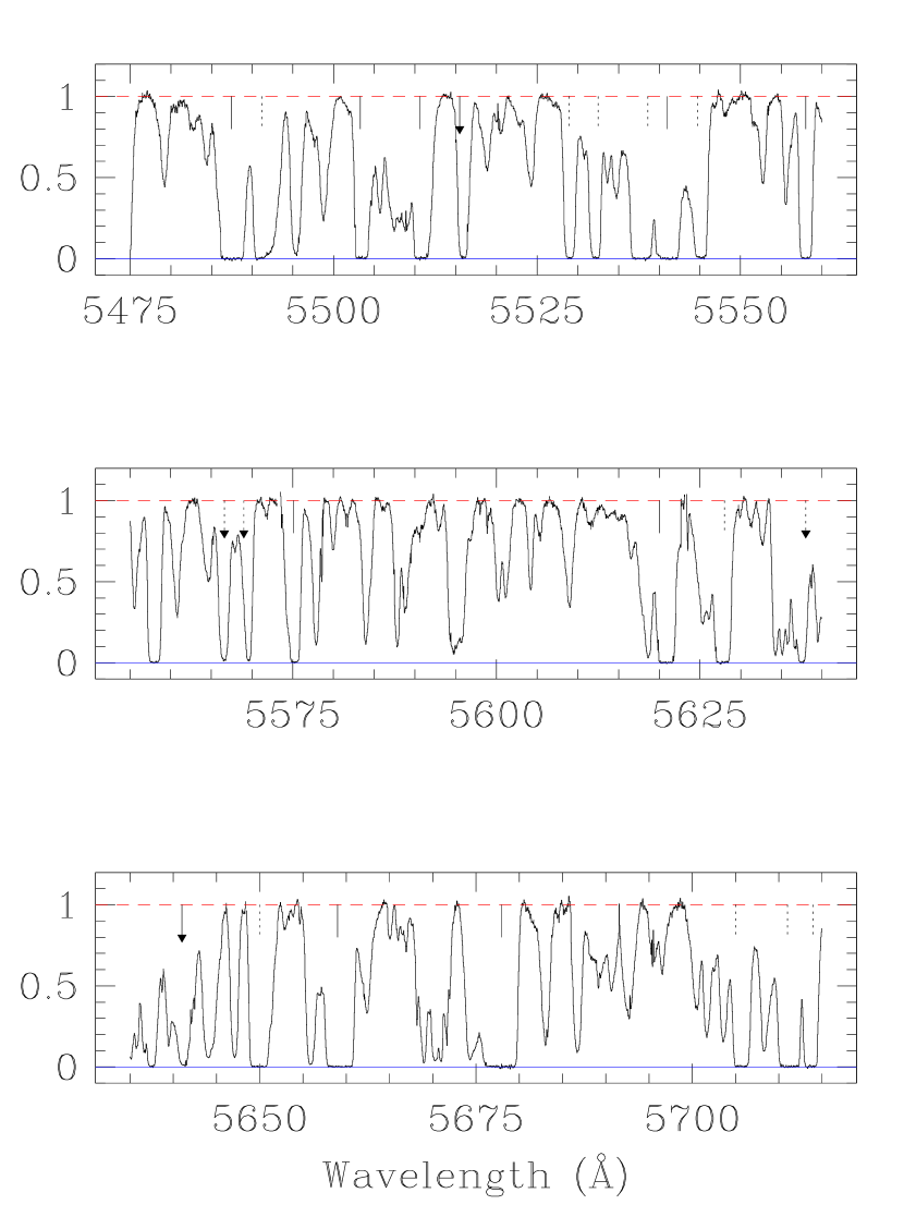
Figure 1: Continued

Figure 1 shows the Ly$\alpha$ forest in APM 08279+5525 between $z_{\rm abs}=3.109$ and 3.701; in this redshift interval there are 58 Ly$\alpha$ lines with $r_{f}<0.025$. However a search for corresponding C IV absorption yielded only 22 C IV systems (38%) at a significance level of $\geq 5\sigma$ .

This apparent discrepancy led us to examine how accurately the $r_{f}<0.025$ cut actually selects Ly$\alpha$ clouds with log $N$(H I)$\geq 14.5$. To this end we used the profile fitting package VPFIT (Webb (1987)) to determine the column density, redshift and $b$ parameter of Ly$\alpha$ lines with $r_{f}<0.025$. We found that although these lines are saturated, in most cases there is sufficient information in the absorption profiles for VPFIT to converge to a reliable solution. Fitting all lines which do not have a flat core at zero residual intensity, showed that 22 out of 58 Ly$\alpha$ lines with $r_{f}<0.025$ do in fact have log $N$(H I)$<14.5$. We have reproduced some examples in Figure 2 and Table 3. The revised sample then consists of 36 Ly$\alpha$ lines with measured log $N$(H I)$>14.5$; 20 of these (56%) have associated C IV systems. This fraction is in good agreement, although somewhat fortuitously, with the value of $58\pm 8$% reported by Songaila & Cowie (1996).

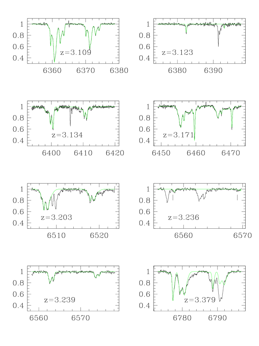
Figure 3: Atlas of C IV doublets associated with Ly$\alpha$ lines in our working region. The $x$-axis is wavelength in Å and the $y$-axis is normalized counts. Thin dotted lines show the profile fits with the parameters listed in Table 2. The weakest C IV systems are indicated with tick marks to guide the eye.

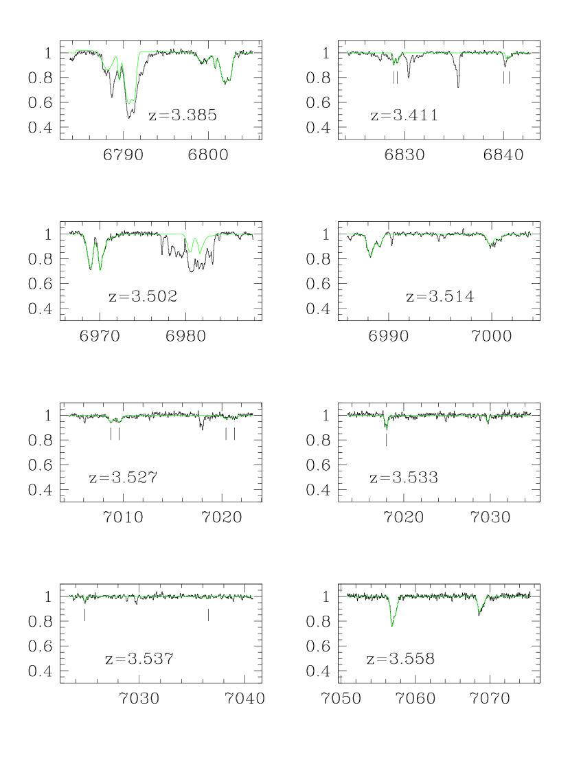
Figure 3: Continued

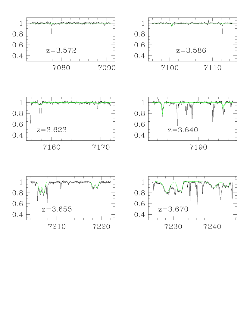
Figure 3: Continued

All of the C IV systems found within our redshift interval were fitted with Voigt profiles using VPFIT (all C IV lines were unsaturated, thus allowing accurate determinations of their column densities) and the model parameter fits for $z$, $N$(C IV), and $b$ are listed in Table 2. Fig 3 is an atlas of the 23 C IV systems whose corresponding Ly$\alpha$ lines lie within our redshift interval; 22 of these have Ly$\alpha$ with $r_{f}<0.025$. Only the 20 C IV systems with a measured log $N$(H I)$>14.5$ are considered in the statistics below.

In order to derive the typical $N$(C IV)/$N$(H I) ratio in Ly$\alpha$ clouds with log $N$(H I) $>14.5$, we follow the procedure used by Cowie et al. (1995). For an H I column density distribution of the form

$$n(N)dN\propto N^{-1-\beta}dN$$ (1)

with $\beta\simeq 0.7$ (Petitjean et al. (1993)), the median $N$(H I) is $2^{\beta}$ times the minimum value or, in our case, $5\times 10^{14}$ cm^-2. Our $5\sigma$ detection limit for C IV$\lambda 1548$ corresponds to $N$(C IV)$=7\times 10^{11}$ cm^-2 for the median $b(C~{}IV)=13.4$ km s^-1 (see Table 2). Since at this detection level approximately half of the Ly$\alpha$ clouds have associated C IV absorption, we deduce a median $N$(C IV)/$N$(H I)$\simeq 1.4\times 10^{-3}$. For comparison, Songaila & Cowie (1996) reported median values of $N$(C IV)/$N$(H I) between $1.6\times 10^{-3}$ and $2.8\times 10^{-3}$.

In Figure 4 we show the column density distribution of C IV lines again assumed to be a power law of the form

$$f(N)dN=BN^{\alpha}dN$$ (2)

where $f(N)$ is the number of systems per column density interval per unit redshift path. The redshift path (used instead of $z$ in order to account for comoving distances) is given by $X(z)={1\over 2}[(1+z)^{2}-1]$ for $q_{0}=0$. A maximum likelihood (e.g. Schechter & Press 1976) fit to the total (unbinned) sample of 20 C IV systems yielded $\alpha=-1.0\pm 0.1$ for column densities in the range $11.74\leq$log $N$(C IV) $\leq 14.25$. This value of $\alpha$, which is shown as a solid line in Figure 4, would indicate a flatter power law distribution than the value $\alpha=-1.5$ (dashed line in Figure 4) deduced by Songaila (1997) from her analysis of a larger sample of 81 C IV absorbers towards seven QSOs. Formally, the difference is significant. A Kolmogorov-Smirnov (K-S) test returns a 76% probability that our data points are drawn from a distribution with $\alpha=-1.0$, but only a $<1$% probability that they arise by chance from a distribution with $\alpha=-1.5$. However, there are significant variations in the statistics of C IV absorbers between different sight-lines in Songaila’s sample and the integral of our power-law distribution, $\sum N(C~{}IV)/\Delta X=2.3\times 10^{14}$ cm^-2, is the same as that reported by Songaila for one of the sight-lines in her study, towards Q0956+122. Thus the difference between our best fitting value of $\alpha$ and that determined by Songaila (1997) may just be due to the limited statistics of the current samples.

5 Ly$\alpha$ Clouds with 13.5 $<$ log $N$(H I)$<$ 14.0

5.1 The stacking method

We now turn to the question of whether Ly$\alpha$ clouds with log $N$(H I)$<14.0$ have a significantly lower metallicity than those with log $N$(H I)$>14.5$. Lu et al. (1998) tackled this problem by stacking together the C IV regions corresponding to $\sim 300$ Ly$\alpha$ lines towards nine QSOs; no significant signal was found in the final composite spectrum. In constructing their sample, Lu et al. targeted column densities in the range $13.5<$ log$~{}N(H~{}I)<14.0$ and, for expediency, assumed that this range corresponds to values of residual flux $0.05<r_{f}<0.38$. Although our statistics are more limited, we can improve on previous analyses by constructing our sample more carefully and by simulating the results of the stacking process for our observed distributions of column densities and $b$-values, as we now discuss.

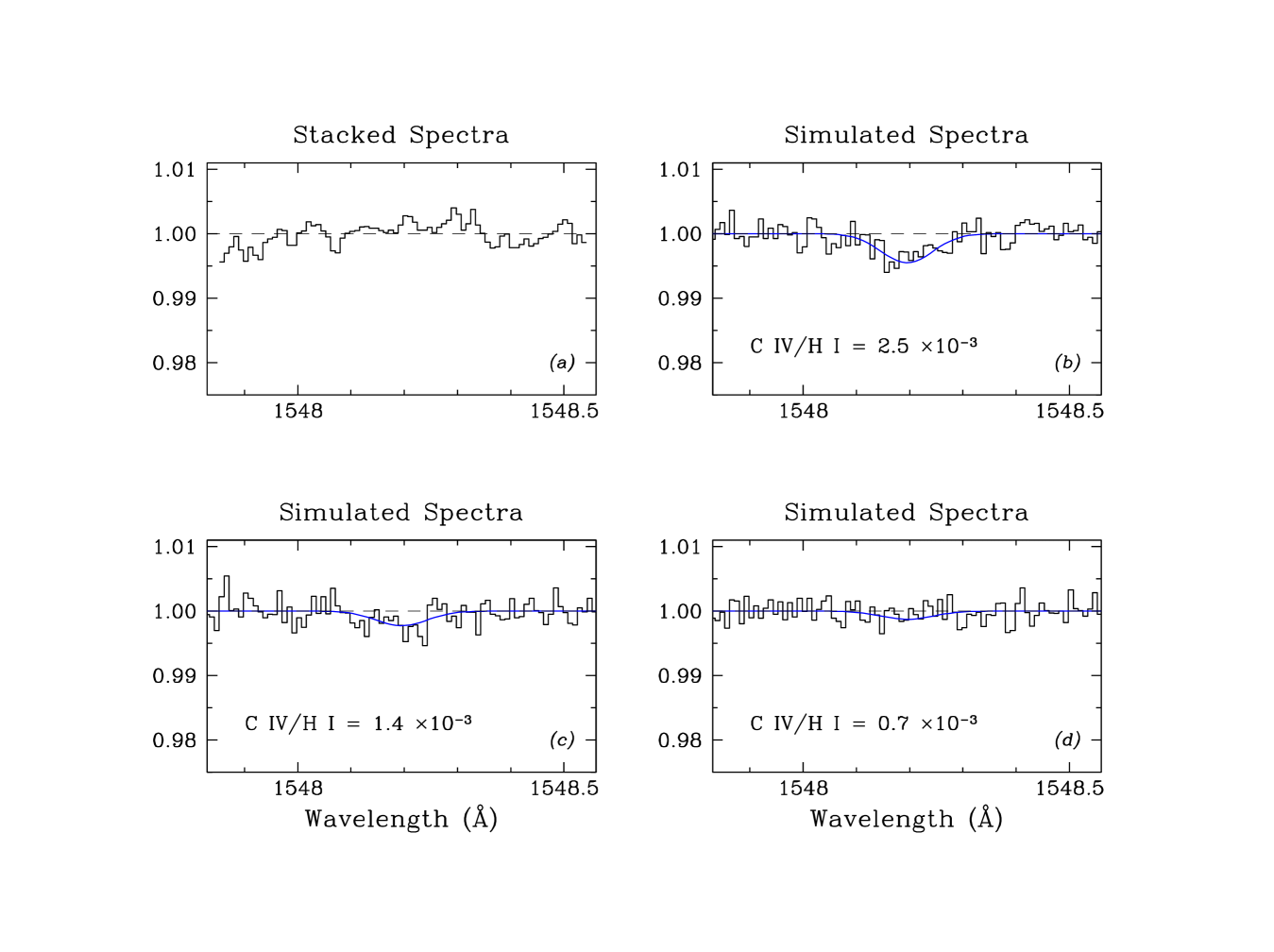
Figure 5: (a): Co-added spectrum obtained by stacking 51 C IV regions corresponding to Ly$\alpha$ lines with $13.5\leq$ log $N$(H I) $\leq 14.0$ . The resulting S/N is 580. (b), (c), and (d): Simulated stacked spectra for different values of $N$(C IV)/$N$(H I), as indicated. The continuous line in each panel shows the noise-free absorption profile for a single C IV line with the mean $N$(C IV). These simulations assumed no redshift difference between C IV and Ly$\alpha$ lines.

We started by using VPFIT to fit all unsaturated Ly$\alpha$ lines in the spectrum of APM 08279+5525 between $z_{abs}=3.109$ and 3.701 . This produced a sample of 86 lines with $13.5<$log $N(H~{}I)<14.0$. Had we selected on the basis of $r_{f}$ rather than $N$(H I), approximately 30% of lines in the desired column density range would have been missed, and 35% of lines outside the range would have been erroneously included. The lines missed are mainly lines with large values of $b$, and lines which are partially blended but for which VPFIT can still satisfactorily recover the individual values of $N$(H I). In the next step we visually inspected the C IV region corresponding to each Ly$\alpha$ line to assess whether it is suitable for stacking; regions contaminated by atmospheric features or blended with other lines were excluded. This produced a final list of 51 C IV$\lambda 1548$ regions and 40 C IV $\lambda 1550$ regions each 7 Å wide, which could be stacked. After reducing each portion of the spectrum to the rest frame using the values of $z_{abs}$ appropriate to each Ly$\alpha$ line (as measured with VPFIT), the regions were summed and renormalized. The final co-added spectrum has S/N = 580 and is reproduced in Figure 5a.

It is clear from Figure 5a that no absorption is detected in the stacked spectrum. In order to assess the significance of this non-detection, we compare the stacked spectrum with that obtained by adding together the same number of C IV lines with strengths predicted for different values of $N$(C IV)/$N$(H I). In performing these simulations we again made use of the available information on the distribution of column densities and $b$-values appropriate to each line, rather than assuming representative values of these quantities, as was done in earlier analyses. Specifically, we simulated the absorption profiles of 51 C IV$\lambda 1548$ lines assigning to each a column density $N$(C IV)_i = $N$(H I)${}_{i}\times A$, where $N$(H I)_i is the neutral hydrogen column density returned by VPFIT for the $i$th Ly$\alpha$ line, and $A$ is the adopted ratio $N$(C IV)/$N$(H I). We repeated the simulations for three values of $A=2.5\times 10^{-3}$ (Cowie & Songaila 1998), $1.4\times 10^{-3}$, the median value deduced here for clouds with log $N$(H I)$\geq 14.5$, and $0.7\times 10^{-3}$, a factor of two lower than our median.

Concerning the value of $b$ to be assigned to each C IV line in the simulations, we could in principle consider two possibilities. If $b$ reflected primarily large-scale motions of the absorbing gas, $b(C~{}IV)_{i}=b(H~{}I)_{i}$. On the other hand, if $b$ has mainly a thermal origin, the $b$-values would scale as the square root of the atomic mass and $b(C~{}IV)_{i}=1/\sqrt{12}\times b(H~{}I)_{i}$. The real situation will be somewhere between these two extremes. Rauch et al. (1996) found mean and median values of $b(C~{}IV)$ near 10 km s^-1 from their analysis of 208 C IV absorption components, and concluded that both thermal motions and bulk motions contribute to the line broadening. Our distribution of $b(C~{}IV)$ for Ly$\alpha$ clouds with log $N$(H I)$\geq 14.5$ has a median value $b(C~{}IV)=13.4$ km s^-1  whereas for $13.5\leq$ log $N$(H I)$\leq 14.0$ we find a median $b(H~{}I)=28.7$. In the simulations we therefore adopted $b(C~{}IV)_{i}\simeq 1/2~{}b(H~{}I)_{i}$, with the implicit assumption that there is no significant change in the distribution of $b$-values with column density.

Theoretical C IV$\lambda 1548$ absorption line profiles were computed in this manner for the 51 Ly$\alpha$ lines in our sample, convolved with the instrumental resolution, and then co-added. The resulting composite profiles, degraded with random noise corresponding to the S/N = 580 of the real stacked data, are shown in Figures 5b, c, and d. Also shown in these panels is the corresponding theoretical absorption profile for the mean $N$(C IV).

The case $A=2.5\times 10^{-3}$ (Figure 5b) produces a composite absorption feature which is significant at the $7\sigma$ level; such a high value of the $N$(C IV)/$N$(H I) ratio would therefore appear to be excluded by our observations. At these low optical depths the equivalent width of the co-added C IV$\lambda 1548$ line scales linearly with $A$. Thus, if the median $A=1.4\times 10^{-3}$ found above for Ly$\alpha$ clouds with log $N$(H I) $\geq 14.5$ also applied at log $N$(H I) $=13.5-14.0$, we may also expect a detectable signal ($4\sigma$, Figure 5c), whereas no composite absorption would be recognized if $A=0.7\times 10^{-3}$ (Figure 5d).

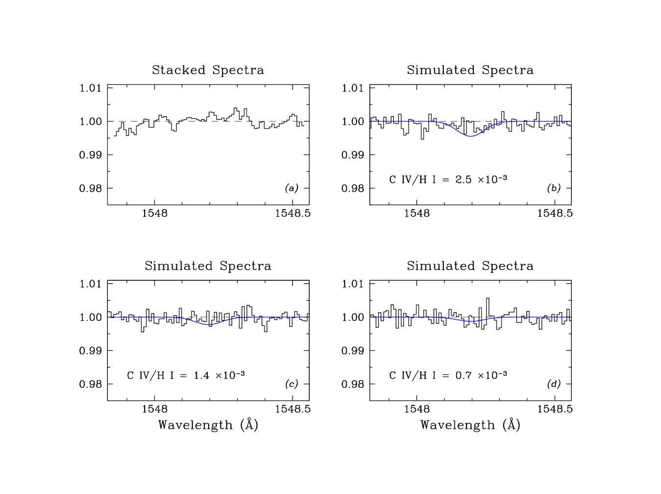
Figure 6: As Figure 5, except that the simulated spectra include allowance for a random redshift difference $\Delta z$ between the centroids of C IV and Ly$\alpha$ absorption. Values of $\Delta z$ were drawn from a Gaussian distribution with $\sigma=27$ km s^-1.

In the above simulations we have assumed that $z(C~{}IV)_{i}=z(H~{}I)_{i}$. However, in reality there is likely to be a dispersion of values of $\Delta z_{i}=z(C~{}IV)_{i}-z(H~{}I)_{i}$. We have already seen that $b(C~{}IV)_{i}\simeq 1/2~{}b(H~{}I)_{i}$, indicative of the fact that Ly$\alpha$ absorption takes place over a wider velocity range than C IV. If we compare the measured values of $z(C~{}IV)_{i}$ and $z(H~{}I)_{i}$ in the 20 Ly$\alpha$ clouds with log $N$(H I) $\geq 14.5$ which show C IV absorption (§4 above), we find a distribution of values of $\Delta z_{i}$ with $\sigma_{z}=4\times 10^{-4}$ which corresponds to a velocity dispersion of 27 km s^-1. We therefore repeated the simulations above assuming that the C IV$\lambda 1548$ lines to be stacked are drawn at random from a Gaussian distribution of $\Delta z_{i}$ with this value of $\sigma$; the results are reproduced in Figures 6b, c, and d.

Clearly, once this redshift dispersion is introduced in the sample, the signal in the stacked spectrum is blurred to the point where it is questionable whether it would be detected even if $N$(C IV)/$N$(H I) $=2.5\times 10^{-3}$. Although the average residual intensity in Figure 6b is less than one, the absorption is so diffuse that it becomes difficult to distinguish it from small fluctuations of the continuum level. We thus seem to have identified a fundamental limitation of the stacking method for the detection of very weak absorption features. Unless it can be shown that $\Delta z$ decreases with log $N$(H I), it would appear that the uncertainty in the exact redshift of the metal lines relative to Ly$\alpha$ casts serious doubt on the interpretation of non-detections in composite spectra, even at a signal-to-noise ratio well in excess of that of the observations reported here. In any case, this probably explains why the first attempts at stacking QSO spectra to search for weak C IV lines (e.g. Lu 1991) underestimated the typical $N$(C IV)/$N$(H I) ratio subsequently measured with HIRES spectroscopy. It is interesting to note in this context that the only case where the stacking method has produced an incontrovertible detection is when Barlow & Tytler (1998) co-added HST FOS spectra to detect C IV associated with Ly$\alpha$ clouds at low redshift ($\langle z\rangle\simeq 0.5$). At the coarse resolution of the FOS spectra—a factor of $>25$ worse than that of HIRES data—the velocity difference between C IV and Ly$\alpha$ becomes a secondary effect.

5.2 Pixel-by-pixel Comparison

Cowie & Songaila (1998) have recently proposed a novel way to look for weak absorption features associated with Ly$\alpha$ forest lines. The method involves constructing cumulative distributions of optical depths for all the pixels in a spectrum where (in this case) C IV $\lambda 1548$ absorption may be found, that is all pixels at wavelengths

$$\lambda_{j}=\frac{1548.195}{1215.670}\times\lambda_{i}$$ (3)

where $\lambda_{i}$ is the wavelength of the $i$th pixel in the Ly$\alpha$ forest. Since no C IV absorption is expected for Ly$\alpha$ pixels with optical depth $\tau{\rm(Ly\alpha)}<0.1$, the distribution of corresponding values of $\tau{\rm(C~{}IV)}$ provides a reference ‘blank’ sample. One can then examine the difference between the distribution of $\tau{\rm(C~{}IV)}$ for a particular range of $\tau{\rm(Ly\alpha)}$ values and the blank sample to determine whether a residual signal is present and indeed Cowie and Songaila (1998) reported excess C IV absorption for all Ly$\alpha$ optical depths, from $\tau{\rm(Ly\alpha)}=20$ to 0.5 .

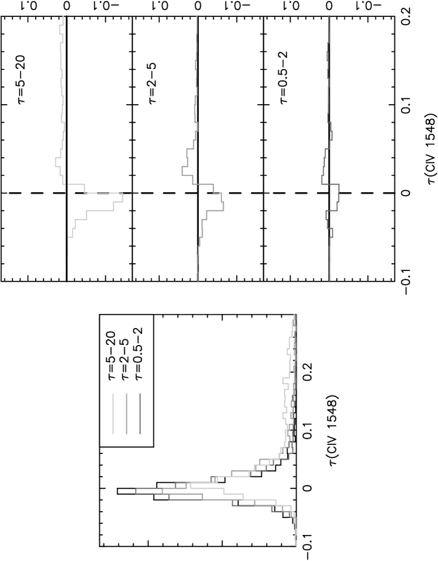
Figure 7: Left: Distribution of C IV optical depths for different ranges of Ly$\alpha$ optical depth, as indicated.  Right: Differential distributions of C IV optical depths, relative to that for $\tau{\rm(Ly\alpha)}<0.1$ where no C IV absorption is expected.

We followed closely the procedure outlined by Cowie & Songaila (1998) in applying their method the spectrum of APM 08279+5525. The results are reproduced in Figure 7, where the left-hand panel shows the distributions of $\tau{\rm(C~{}IV)}$ for the same three ranges of $\tau{\rm(Ly\alpha)}$ considered by Cowie & Songaila. The differential distributions relative to the blank sample are shown in the right-hand panel; here the deficit of pixels with negative values of $\tau{\rm(C~{}IV)}$ and the excess of pixels with positive $\tau{\rm(C~{}IV)}$ give an ‘S wave’ pattern which is indicative of C IV absorption associated with Ly$\alpha$ forest lines. As can be seen from the Figure, we confirm the finding by Cowie & Songaila of a C IV signal in all three intervals of $\tau{\rm(Ly\alpha)}$ considered.

It is of interest, of course, to ask how changes in the $N$(C IV)/$N$(H I) ratio would be reflected in the optical depth distributions shown in Figure 7. We are in a good position to explore this question having quantified the absorption parameters of the entire Ly$\alpha$ forest in APM 08279+5525. To this end, we simulated the C IV absorption associated with 375 Ly$\alpha$ lines for which VPFIT returned values of $N$(H I), $z$, and $b$, and applied Cowie and Songaila’s technique to determine the distributions of $\tau{\rm(Ly\alpha)}$ and $\tau{\rm(C~{}IV)}$. Since the aim is to test whether there is a sudden change in the metallicity of Ly$\alpha$ clouds at low optical depths, we considered two possibilities:

(1) $N$(C IV)/$N$(H I)$=2.5\times 10^{-3}$ for all values of $N$(H I); and

(2) a drop in $N$(C IV)/$N$(H I) by a factor of 10 for $N$(H I)$<14.0$ .

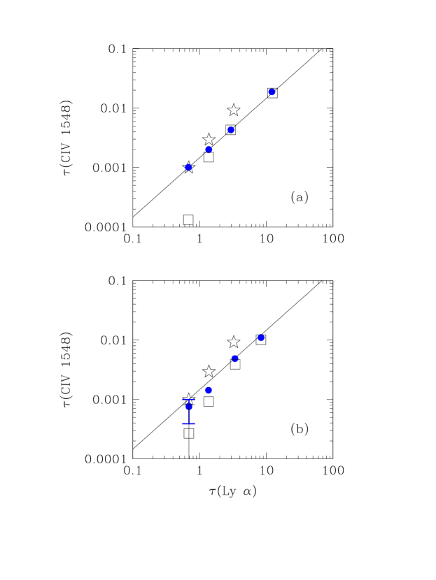
Figure 8: Median values of optical depth of C IV $\lambda 1548$ for different ranges of Ly$\alpha$ optical depth. The open star symbols are the values measured in the HIRES spectrum of APM 08279+5525; no value is plotted for the bin $\tau$(Ly$\alpha$)$=5-20$ because the residual intensity in these pixels is too low to measure the optical depth without reference to higher order Lyman lines. The filled circles and open squares show the results of the simulations described in the text. The filled circles are for the case where $N$(C IV)/$N$(H I)$=2.5\times 10^{-3}$ (straight line) was assumed throughout, whereas the open squares are for simulations where a sudden drop by a factor of 10 in $N$(C IV)/$N$(H I) was introduced at log $N$(H I)$<14.0$ . The top and bottom panels correspond respectively to the ‘ideal’ and ‘realistic’ simulations discussed in the text. In the lower panel the error bars (only plotted if they are larger than the symbols) show the dispersion in the results when the same simulation was repeated twelve times.

We carried out the simulations for two cases which we term ‘ideal’ and ‘realistic’. In the ideal case, we did not include the effects of noise (that is, we assumed infinitely high S/N) and we adopted $b(C~{}IV)_{i}=b(H~{}I)_{i}$ and $z(C~{}IV)_{i}=z(H~{}I)_{i}$ . In the realistic case, we introduced random noise in the simulations to reproduce the S/N = 80 typical of our HIRES data. We also assumed $b(C~{}IV)_{i}=1/2~{}b(H~{}I)_{i}$ and a dispersion of values $\Delta z_{i}=z(C~{}IV)_{i}-z(H~{}I)_{i}$ with $\sigma_{z}=4\times 10^{-4}$ as found for Ly$\alpha$ lines with log $N{\rm(H~{}I)}\geq 14.5$ (§5.1) . The results of these simulations are reproduced in Figure 8. Since the assumed drop in the $N$(C IV)/$N$(H I) ratio at $N$(H I)$<14.0$ (case 2) would affect primarily pixels with $\tau$(Ly$\alpha$) $\lower 2.15277pt\hbox{$\;\buildrel<\over{\sim}\;$}1$, for clarity we show the results at low optical depths in two subsets: $\tau$(Ly$\alpha$) $<1$ and $1\leq\tau$(Ly$\alpha$) $\leq 2$ .

The top panel in Figure 8 shows that in the ‘ideal’ case the optical depth method developed by Cowie and Songaila (1998) would indeed be sensitive to changes in the Carbon abundance of Ly$\alpha$ clouds (open squares). Under more realistic conditions (bottom panel), however, the break below $\tau$(Ly$\alpha$)$\simeq 1$ is softened, primarily by the effect of noise which moves pixels with $1\leq\tau$(Ly$\alpha$) $\leq 2$ into the lower optical depth interval and vice versa. Furthermore, at the typical S/N of the present data, the error associated with the lowest $\tau$(C IV) bin is so large that the two cases considered (filled dot and open square) can no longer be distinguished with confidence. Although the data (open star) apparently favour a constant $N$(C IV)/$N$(H I), we feel that the existence of a break below $\tau$(Ly$\alpha$)$\simeq 1$ can only be tested reliably with higher S/N observations.

6 Summary and Conclusions

We have presented a high resolution ($\sim$ 6 km s^-1) and high S/N ($\sim 80$) spectrum of the ultraluminous BAL QSO APM 08279+5255 obtained with HIRES on the Keck I telescope. These data, which have a sensitivity to C IV $\lambda\lambda 1548,1550$ lines with rest frame equivalent widths as low as $\sim$3 mÅ ($5\sigma$), have been analyzed with a view to reassessing the metallicity of the Ly$\alpha$ forest at $z\simeq 3.4$. Our principal results are as follows.

In agreement with previous analyses, we find that approximately 50% of Ly$\alpha$ clouds with log $N$(H I)$\geq 14.5$ have associated C IV systems with log $N$(C IV)$\lower 2.15277pt\hbox{$\;\buildrel>\over{\sim}\;$}12.0$; we deduce a median $N$(C IV)/$N$(H I)$\simeq 1.4\times 10^{-3}$. However, we point out that the criterion previously adopted to identify such Ly$\alpha$ clouds—a residual flux in the line core $r_{f}<0.025$—is an inadequate approximation which can miss a significant proportion of the lines. Even though the absorptions are close to saturation, profile fitting methods which simultaneously determine the column density and velocity dispersion of the absorbers are preferable for a clean definition of the sample (for data of sufficiently high S/N and resolution, such as those presented here).

We have stacked the C IV$\lambda 1548$ regions corresponding to 51 Ly$\alpha$ lines with $13.5\leq$ log $N$(H I) $\leq 14.0$ but find no detectable signal in the composite spectrum. In order to understand the significance of this null result, we have performed simulations in which we stack 51 synthetic C IV$\lambda 1548$ lines with absorption parameters resembling as closely as possible those of the lines we are trying to detect. Specifically, each C IV line to be stacked was assigned values of column density and velocity dispersion scaled directly from those of the corresponding Ly$\alpha$ line. These simulations show that we should be able to detect a marginally significant ($4\sigma$) absorption feature in the co-added spectrum if $N$(C IV)/$N$(H I)$=1.4\times 10^{-3}$, as in clouds with log $N$(H I) $\geq 14.5$, provided that there is no random difference $\Delta z$ between the redshifts of C IV and Ly$\alpha$.

However, when such a difference is introduced in the simulations the co-added signal is effectively washed out to the point where it can no longer be recognized. This is the case even for a relatively small dispersion of values of $\Delta z$ ($\sigma=27$ km s^-1) which is entirely plausible given the observed distribution of $\Delta z$ in the higher column density clouds where C IVis detected. We propose that this uncertainty in the exact registration of weak signals is a serious problem which ultimately limits the usefulness of stacking procedures.

We also analysed our data with the pixel-by-pixel optical depth method recently developed by Cowie & Songaila (1998) and, in agreement with these authors, we do find a signal indicative of C IV absorption in Ly$\alpha$ clouds with optical depths as low as $\tau{\rm(Ly\alpha)}=0.5-2$ . However, our simulations show that a higher S/N than achieved up to now is required to detect with confidence even a marked break in the $N$(C IV)/$N$(H I) ratio below log $N$(H I)$\lower 2.15277pt\hbox{$\;\buildrel<\over{\sim}\;$}14.0$ .

We conclude that the question of whether the abundance of Carbon in the Ly$\alpha$ forest is uniform at all column densities has yet to be fully answered. Probably this question is best addressed by pushing the detection limit for C IV absorption lines below the limits reached so far. Thanks to the extraordinary luminosity of APM 0827+5255 this approach is now feasible with a concerted effort of HIRES observations.

7 Acknowledgements

The authors would like to express their gratitude to both Craig Foltz and Michael Rauch for obtaining some of the observations presented in this paper. We are also grateful to Tom Barlow for his help using HAR and to Bob Carswell, Jim Lewis and Jon Willis for their generous help with various stages of data reduction. SLE would like to thank the University of Victoria and the University of Washington for hosting visits and especially Arif Babul and Chris Pritchet at the University of Victoria for financial support. SLE acknowledges PPARC for her PhD studentship and WLWS acknowledges support from NSF Grant AST-9529073.

Figure 2: Examples of Ly$\alpha$ absorption lines with $r_{f}<0.025$ and log $N$(H I)$<14.5$. Theoretical line profiles computed with VPFIT are shown as a continuous line in each panel. Parameters of the fits are collected in Table 2.

Figure 4: Column density distribution of C IV absorbers in APM 08279+5255. The data have been grouped into bins of width 0.5 in log $N$(C IV) for display purposes only. The top panel shows the cumulative distribution and the bottom panel is the differential. A maximum likelihood analysis of the distribution, assumed to be a power-law of the form $f(N)dN=BN^{\alpha}dN$, returned a best fit index $\alpha=-1.0$ indicated by the solid line. The dashed line in the bottom panel ($\alpha=-1.5$) is the slope reported by Songaila (1997) for her larger sample.

Table 1: Journal of HIRES Observations of APM 08279+525

Date	Integration time (s)	Wavelength range (Å)	Typical S/N
April 1998	1800	4400 – 5945	15
April 1998	1800	4400 – 5945	15
April 1998	1800	4400 – 5945	15
April 1998	1800	4400 – 5945	15
May 1998	2700	4410 – 5950	25
May 1998	2700	4400 – 5945	25
May 1998	900	5440 – 7900	30
May 1998	3000	5440 – 7900	60
May 1998	3000	5440 – 7900	60
May 1998	3000	5475 – 7830	55
May 1998	3000	5475 – 7830	55
May 1998	3000	6765 – 9150	50
May 1998	3000	6850 – 9250	50
Summed Total	31 500	4400 – 9250	30 –150

Table 2: Details of Absorption Components Fitted to Each C IV System.

System No.	Redshift	log $N$(C IV)	$b$ (km s-1)	Comments
C1	3.10742	12.50	17.2
	3.10769	12.89	6.7
	3.10791	12.62	10.5
	3.10841	12.50	3.7
	3.10850	13.74	25.7
	3.10952	12.67	9.2
	3.10966	13.21	28.2
	3.11027	12.78	11.8
C2	3.12252	12.50	7.8	log $N$(H I)$<$ 14.5
C3	3.13296	12.98	39.0
	3.13363	12.30	22.5
	3.13367	12.97	12.4
	3.13416	13.23	14.9
	3.13505	12.33	9.6
C4	3.16966	13.35	38.5
	3.16976	12.90	16.3
	3.17039	12.69	9.8
	3.17117	13.24	58.6
C5	3.17205	12.13	5.7
	3.17233	13.18	6.7
	3.17237	12.34	15.8
	3.17264	12.34	15.8
	3.17330	12.19	13.3
C6	3.20266	12.23	9.9
	3.20300	12.76	8.8	Some of 1548 Å lines blended
	3.20345	13.55	58.9
	3.20359	12.84	15.8
C7	3.23618	12.04	8.4
C8	3.23895	12.98	19.4
	3.23950	12.58	10.5
C9	3.37677	12.24	24.5	Some blending in both doublet lines
	3.37757	12.81	6.5
	3.37770	13.28	19.7
	3.37882	12.37	10.8
	3.37891	13.24	22.5
	3.37969	13.56	45.4
	3.37969	12.89	17.0
C10	3.38456	13.13	36.0	1548 Å line is blended with the 1550 Å
	3.38543	12.65	7.4	line from the previous system.
	3.38616	13.51	25.9
	3.38660	13.02	13.4
C11	3.41088	11.90	1.5	1550 Å line is blended.
	3.41111	12.35	11.9
C12	3.50125	13.01	16.8	Some blending in both doublet lines
	3.50141	12.39	9.9
	3.50204	12.24	5.3
	3.50209	13.08	22.6
	3.50281	12.39	32.8
C13	3.51380	12.88	17.1
	3.51436	12.54	14.8
C14	3.52706	12.24	13.1
	3.52760	12.33	16.9
C15	3.53303	12.37	8.9
C16	3.53744	11.63	2.4	Very weak, 1550 Å line barely visible
C17	3.55811	12.85	11.5
	3.55842	12.63	12.7
C18	3.57168	11.79	6.6
C19	3.58630	12.02	5.5
C20	3.62314	11.97	9.1
	3.62339	11.76	5.4
C21	3.63954	12.47	3.0	1550 Å line is blended
	3.63968	12.09	1.9
C22	3.65458	12.90	14.3	1548 Å line is blended
	3.65514	12.89	13.9
C23	3.66863	12.88	89.3	Satisfactory fit, although slight blending
	3.66892	13.22	36.9
	3.67082	12.97	21.4
	3.67131	12.81	15.3

Table 3: Parameter Fits for Absorption Lines Shown in Figure 2

Line No.	Redshift	log $N$(H I)	$b$ (km s-1)
1	3.34577	14.18	23.6
2	3.49289	14.13	25.5
3	3.49618	14.28	27.8
4	3.57899	14.21	28.3
5	3.58146	14.08	22.7

References

- Barlow & Tytler (1998) Barlow, T. A. & Tytler, D. 1998, AJ, 115, 1725
- Bi & Davidsen (1997) Bi, H. & Davidsen, A. F. 1997, ApJ, 479, 523
- Carswell et a.l (1991) Carswell, R. F., Lanzetta, K., Parnell, C. H., & Webb, J. K. 1991, ApJ, 371, 36
- Cen et al. (1994) Cen, R., Miralda-Escudé, J., Ostriker, J. P., & Rauch, M. 1994, ApJ, 437, L9
- Cowie & Songaila (1998) Cowie, L. L., & Songaila, A. 1998, Nature, 394, 44
- Cowie et al. (1995) Cowie, L. L., Songaila, A., Kim, T.-S., & Hu, E. 1995, AJ, 109, 1522
- Downes et al. (1999) Downes, D., Neri, R., Wilkind, T., Wilner, D. J., & Shaver, P. 1999, ApJL submitted (astro-ph/9810111)
- Ellison et al. (1999) Ellison, S. L., Lewis, G. F., Pettini, M., Sargent, W. L. W., Chaffee, F. H., Foltz, C. B., Rauch, M., & Irwin, M. J. 1999, PASP, in preparation
- Gnedin (1998) Gnedin, N. Y. 1998, MNRAS, 294, 407
- Gnedin & Ostriker (1997) Gnedin, N. Y., & Ostriker, J. P. 1997, ApJ, 486, 581
- Hellsten et al. (1997) Hellsten, U., Davé, R., Hernquist, L., Weinberg D. H., & Katz, N. 1997, ApJ, 487, 482
- Hernquist et al. (1996) Hernquist, L., Katz, N., Weinberg, D. H., & Miralda-Escudé, J. 1996, ApJ, 457, L51
- Irwin et al. (1998) Irwin, M. J., Ibata, R. A., Lewis, G. F., & Totten, E. J. 1998, ApJ,505, 529
- Ledoux et al. (1998) Ledoux, C., Theodore, B., Petitjean, P., Bremer, M. N., Irwin, M. J., Ibata, R. A., Lewis, G. F., & Totten, E. 1998, A&A, 339, L77
- Lu (1991) Lu, L. 1991, ApJ, 379, 99
- Lu et al. (1998) Lu, L., Sargent, W. L. W., Barlow, T. A., & Rauch, M. 1998, in preparation (astro-ph/9802189)
- Lynds (1971) Lynds, R. 1971, ApJ, 164, L73
- Meyer & York (1987) Meyer, D. M., & York D. G. 1987, ApJ, 315, L5
- Norris, Peterson & Hartwick (1983) Norris, J., Peterson, B. A., & Hartwick, F. D. A. 1983, ApJ, 273, 450
- Ostriker & Gnedin (1996) Ostriker, J. P., & Gnedin N. Y. 1996, ApJ, 472, L63
- Petitjean, Mucket & Kates (1995) Petitjean, P., Mücket, J. P., & Kates R. E. 1995, A&A, 295, L9
- Petitjean et al. (1993) Petitjean, P., Webb, J. K., Rauch, M., Carswell, R. F., & Lanzetta, K. 1993, MNRAS, 262, 499
- Rauch (1998) Rauch, M. 1998, ARA&A, 36, 267
- Rauch, Haehnelt & Steinmetz (1997) Rauch, M., Haehnelt, M. G., & Steinmetz, M. 1997, ApJ, 481, 601
- Rauch et al. (1996) Rauch, M., Sargent, W. L. W., Womble, D. S., & Barlow, T. A. 1996, ApJ, 467, L5
- Sargent et al. (1980) Sargent W. L. W., Young, P.J., Boksenberg, A., & Tytler, D. 1980, ApJS, 42, 41
- Schechter & Press (1976) Schechter, P., & Press W. H. 1976, ApJ, 203, 557
- Songaila (1998) Songaila, A. 1997, ApJL, 490, L1
- Songaila & Cowie (1996) Songaila, A., & Cowie, L. L. 1996, AJ, 112, 335
- Tytler et al. (1995) Tytler, D., Fan, X.-M., Burles, S., Cottrell, L., Davis, C., Kirkman, D., & Zuo, L. 1995, QSO Absorption Lines, ed. G. Meylan (Garching, ESO), 289
- Vogt et al. (1994) Vogt, S. S. 1992, in ESO Conf. and Workshop Proc 40, High Resolution Spectroscopy with the VLT, ed. M.-H. Ulrich (Garching: ESO), 223
- Webb (1987) Webb J. K. 1987, PhD thesis, University of Cambridge