The Axisymmetric Pulsar Magnetosphere

Abstract

We present, for the first time, the structure of the axisymmetric force–free magnetosphere of an aligned rotating magnetic dipole, in the case in which there exists a sufficiently large charge density (whose origin we do not question) to satisfy the ideal MHD condition, ${\bf E\cdot B}=0$, everywhere. The unique distribution of electric current along the open magnetic field lines which is required for the solution to be continuous and smooth is obtained numerically. With the geometry of the field lines thus determined we compute the dynamics of the associated MHD wind. The main result is that the relativistic outflow contained in the magnetosphere is not accelerated to the extremely relativistic energies required for the flow to generate gamma rays. We expect that our solution will be useful as the starting point for detailed studies of pulsar magnetospheres under more general conditions, namely when either the force-free and/or the ideal MHD condition ${\bf E\cdot B}=0$ are not valid in the entire magnetosphere. Based on our solution, we consider that the most likely positions of such an occurrence are the polar cap, the crossings of the zero space charge surface by open field lines, and the return current boundary, but not the light cylinder.

1 Introduction

The issue of the structure of neutron star magnetospheres, roughly thirty years from the seminal paper of Goldreich & Julian (1969, hereafter GJ) which outlined its basic physics, remains still open. The discovery of radiation emission from radio to gamma-rays with the pulsar period has motivated the modification of the original GJ model to include features, such as charge gaps, which would lead to the acceleration of particles necessary to produce the observed radiation.

Thus, the ubiquitous presence of high energy radiation from pulsars, in agreement with simple scaling laws (Harding 1981) which make no particular demands on the magnetic field structure, has prompted a number of authors to suggest that the gamma-ray emission results from an unavoidable violation of the ‘assumption of strictly dissipation–free flow would lead to singularities in both the flow and the magnetic field, occuring a short distance beyond the light–cylinder’ (Shibata 1995; Mestel & Shibata 1994). Such suggestions were corroborated by solutions in which the field lines appeared exhibiting kinks and discontinuities which have been presented occasionally in the literature (e.g. Michel 1982; Sulkanen & Lovelace 1990). Based on the conviction that such singularities might simply reflect the shortcomings of our numerical methods and not the physical path nature chooses, we have decided to investigate the issue ourselves. Our original hope was that an exact solution of the magnetohydrodynamic (MHD) structure of a pulsar magnetosphere would provide also the detailed dynamics of the acceleration of the associated MHD wind which could then resolve the issue of high energy emission from these objects.

As often done in the literature, we will work in the framework of ideal (dissipation–free) magnetohydrodynamics, and will assume that dissipation effects are minor perturbations to the global picture that we will present. We do acknowledge that this idealized picture will not be valid in the presence of physical magnetospheric instabilities (see discussion below), but assuming for the moment that such instabilities are absent, we can justify our approach as follows (e.g. Bogovalov 1997): The gravitational field of an unmagnetized neutron star would reduce a thermally supported atmosphere to a height of a few centimeters and the star would be surrounded by an effective vacuum. Real stars, however, are magnetized and rotation generates huge electric fields which, not only pull charged particles from the surface, but also accelerate them in curved trajectories, generating thus curvature photons which produce electron–positron pairs in the curved magnetic field. An electromagnetic cascade develops within a few stellar radii, and the density of plasma increases up to the point that it becomes high enough to screen the electric field component parallel to the magnetic field. This mechanism is obviously self–regulating. Wherever the density of plasma drops below the absolute minimum required to short–out the parallel component of the electric field, ‘gaps’ will develop, inside which ${\bf E\cdot B}\neq 0$, and the electromagnetic cascade mechanism will regenerate the missing charges.

The condition that ${\bf E\cdot B}=0$ is precisely the condition of ideal MHD, and it will be a valid approximation in the study of the magnetosphere over length scales much larger than the size of the various ‘gaps’. We will further assume that the main stresses in the magnetosphere are magnetic and electric (with inertial and gravitational ones being negligible, at least near the surface of the star), and a valid magnetospheric model will be one where

$$\frac{1}{c}{\bf J\times B}+\rho_{e}{\bf E}=0\ .$$ (1)

Here, ${\bf J}$, ${\bf B}$, and ${\bf E}$ are the electric current density, magnetic and electric fields respectively; and $\rho_{e}=\nabla\cdot{\bf E}/(4\pi)$ is the electric charge density in the magnetosphere. We need to note that this simplifying working assumption is not valid in the neutron star interior (on to which the magnetic field is anchored), and in singular magnetospheric regions (current sheets subject to non–vanishing Maxwell stresses which must be balanced by a thermal pressure). As we will see, we do not have to worry about these regions as long as they are self–consistently treated as boundaries in our problem. More problematic, however, is the force–free assumption, namely that the inertial effects associated with the plasma outlflow are generally small. This assumption may actually be valid in the case of relatively fast rotating, young neutron stars, as in this case the luminosity associated with the gamma ray emission is only a small fraction of the power associated with the spin down of the neutron star through the magnetic torques; (Arons 1981; Daugherty & Harding 1982; Cheng, Ho & Ruderman 1986); however, for older, slower rotating neutron stars for which the radiative efficiency gets close to 1 (Harding 1981), we expect this assumption to be violated. Since little progress has been done in the study of the general problem when matter inertia is not negligible (e.g. Camenzind 1986), we have decided to study the force–free case, bearing in mind that our solution can only serve as a first approximation to the physical one.

Having presented our assumptions and their limitations, let us now investigate more closely what eq. (1) and the assumption of ideal MHD imply about the overall structure of the rotating neutron star magnetosphere.

2 The pulsar equation

A convenient approach in steady–state axisymmetric MHD is to work with the flux function $\Psi$ defined through

$${\bf B_{p}}=\frac{\nabla\Psi\times\hat{\phi}}{R}\ ,$$ (2)

where, $\bf B_{p}$ is the poloidal ($R,Z$) component of the magnetic field in a cylindrical coordinate system ($R,\phi,Z$). Magnetic field lines lie along magnetic flux surfaces of constant $\Psi$. At each point, $\Psi$ is proportional to the total magnetic flux contained inside that point; it is also related to the $\phi$ component of the vector potential. Ideal force–free MHD requires that

$$B_{\phi}=\frac{A(\Psi)}{R}\ ,$$ (3)

where $A(\Psi)$ is a yet to be determined function. Obviously, the poloidal electric current $I\equiv cA/2$ is also a function of $\Psi$, which means that poloidal electric currents are required to flow along (and not across) flux surfaces. Note that this does not in general imply that the electric currents flow along magnetic field lines, since the electric term in eq. (1) cannot in general be neglected. In fact, using eq. (4) (below), one can see that the currents are a sum of a current along the total field plus the convection current due to corotation of the space charge density. Finally, the electric field is given by

$${\bf E}=\frac{R\Omega}{c}{\bf B_{p}}\times\hat{\phi}\ ,$$ (4)

and is clearly perpendicular to ${\bf B}$. $\Omega$ is the angular velocity of rotation of the neutron star on to which the magnetosphere is anchored, and can directly be thought of as the angular velocity of rigid rotation of the magnetic field lines (not of the magnetospheric plasma!). Eq. (1) can now be written in the equivalent form

$$(1-x^{2})\left(\frac{\partial^{2}\Psi}{\partial x^{2}}-\frac{1}{x}\frac{\partial\Psi}{\partial x}+\frac{\partial^{2}\Psi}{\partial z^{2}}\right)-2x\frac{\partial\Psi}{\partial x}=-R_{LC}^{2}AA^{\prime}\ ,$$ (5)

where we have introduced the convenient notation $x\equiv R/R_{LC}$ and $z\equiv Z/R_{LC}$, with $R_{LC}\equiv c/\Omega$ the distance from the axis where a particle corotating with the star would rotate at the speed of light (the so called ‘light cylinder’); and $(\ldots)^{\prime}\equiv{\rm d}/{\rm d}\Psi$. Eq. (5) is the well known pulsar equation (Michel 1973a; Scharlemann & Wagoner 1973). Solutions to this equation have been found for specific functional forms of the current distribution $A(\Psi)$. Michel has presented solutions for $A=$ const. and $A=-2\Psi$ for which this equation becomes linear and the usual techniques can be applied to derive the form of the field geometry for $x\leq 1$. Michel has also presented solutions for a quadratic form of $A(\Psi)$ corresponding to a magnetic monopole solution.

One can check that, when this equation is satisfied, the space charge (or GJ charge) density is conveniently given by

$$\rho_{e}=\left(\frac{\Omega}{4\pi c}\right)\frac{-2B_{z}+AA^{\prime}}{1-x^{2}}\ .$$ (6)

Eq. (5) is elliptic, and according to the theory of elliptic equations (albeit the linear ones), the solution at all $x$ and $z$ is uniquely determined when one specifies the values of either $\Psi$ (Dirichlet boundary conditions) or the normal derivative of $\Psi$ (Neumann boundary conditions) along the boundaries, i.e. along the axis $x=0$, the equatorial plane $z=0$, and infinity (as one expects, and as we will see in practice, the boundary conditions at infinity will not affect the solution near the origin and the light cylinder). Unfortunately, this procedure does not work since eq. (5) is singular at the position of the light cylinder $x=1$. The singularity at $x=1$ imposes the important constraint that

$$\frac{\partial\Psi}{\partial x}=\frac{1}{2}AA^{\prime}\ ,$$ (7)

at all points along the light cylinder, and as a result, not all distributions of electric current along the open field lines $A=A(\Psi)$ will lead to solutions which cross the light cylinder without kinks or discontinuities. In fact, as we will see, there exists a unique (?) distribution $A=A(\Psi)$ which allows for the continuous and smooth crossing of the light cylinder.

How can one determine what is the distribution of $A=A(\Psi)$? One sees directly that eq. (7) has precisely the form of a boundary condition along the light cylinder which will allow for the solution of eq. (5) inside and outside the light cylinder. In other words, eq. (7) determines the normal derivative of $\Psi$ along the light cylinder, when $A=A(\Psi)$ is known, which can be used to solve the original elliptic equation both inside and outside $x=1$. The inside solution will yield the distribution of $\Psi(x=1^{-},z)$, the outside solution the distribution of $\Psi(x=1^{+},z)$, and in general, $\Psi(x=1^{-},z)$ will not be equal to $\Psi(x=1^{+},z)$, unless of course one is ‘lucky enough’ to try the correct distribution of $A(\Psi)$. To the best of our knowledge, all to date efforts to solve the distorted dipole magnetosphere lead to the conclusion that ‘the assumption of strictly dissipation–free flow would lead to singularities in the magnetic field, occuring a short distance beyond the light–cylinder’ (Mestel & Shibata 1994). Several unsuccessful attempts to solve eq. (5) in all space, have concluded in favor of the ‘inevitability of the break–down of continuity and smoothness’ of these solutions.

On the other hand, motivated by the fact that the singularity at the light cylinder is none other than the relativistic unique generalization of the familiar Alfvén point of the non–relativistic theory (Li & Melrose 1994; Camenzind 1986) under force–free conditions, we were more optimistic in that such a continuous and smooth solution actually exists; we considered the fact that it had not been found not a sufficient argument against its existence. We are all too familiar with the difficulties associated with the continuous and smooth crossing of the non–relativistic Alfvén singular point (Contopoulos 1994, 1995) and no one believes anymore early solutions which are either discontinuous or show kinks at or around the position of the Alfvén point. Moreover, smooth and continuous solutions of the special relativistic problem exist in a couple of idealized cases: the simple monopole (Michel 1991), a collimated proto stellar jet (Fendt, Camenzind, Appl 1995), and a differentially rotating self–similar disk–wind (Li, Chiueh & Begelman 1992; Contopoulos 1994). We really cannot see why would the relativistic Alfvén point of the rotating dipole problem fare otherwise.

3 The Numerical Procedure

We have, therefore, set out to obtain the solution of the force–free rotating relativistic dipole problem in all space, without kinks or discontinuities on or around the light cylinder, using the following relaxation type technique:

1. We chose some (any) initial trial electric current distribution (the one which corresponds to the relativistic monopole solution yields easier numerical convergence).

2. We then solve the problem both inside and outside the light cylinder, and thus obtain the two distributions $\Psi(x=1^{-},z)$ and $\Psi(x=1^{+},z)$ along the light cylinder, which in general differ.

3. We correct for the distribution of $A(\Psi)$ along field lines which cross the light cylinder as follows: At each point $z$ of the light cylinder correspond values of $AA^{\prime}(\Psi(x=1^{-},z))$ and $AA^{\prime}(\Psi(x=1^{+},z))$. From them, we obtain the new distribution

   $$AA^{\prime}|_{\rm new}(\Psi) = \mu_{1}AA^{\prime}(\Psi(x=1^{-},z))+\mu_{2}AA^{\prime}(\Psi(x=1^{+},z))$$ (8)

   $$+\mu_{3}[\Psi(x=1^{+},z)-\Psi(x=1^{-},z)]\ ,$$

   $${\rm for}\ \Psi=\frac{1}{2}[\Psi(x=1^{-},z)+\Psi(x=1^{+},z)]\ ,$$ (9)

   with weight factors $\mu_{1}+\mu_{2}=1$, and $\mu_{3}\ll 1$ chosen empirically in order to facilitate numerical convergence. Eq. (8) can be seen as an equation $AA^{\prime}|_{\rm new}=AA^{\prime}|_{\rm new}(\Psi)$, which is solved to yield the distribution $A|_{\rm new}(\Psi)$, with the boundary condition $A|_{\rm new}(\Psi=0)=0$. Obviously we also require that $A=0$ along closed field lines.

4. We repeat steps 1 to 3 until the difference $[\Psi(x=1^{+},z)-\Psi(x=1^{-},z)]$ becomes numerically negligible along all points of the light cylinder.

Obviously, at that point, the solution will be both continuous (i.e. $\Psi(x=1^{-},z)=\Psi(x=1^{+},z)$), and smooth (i.e. $\partial\Psi/\partial x|_{x=1^{-}}=\partial\Psi/\partial x|_{x=1^{+}}=AA^{\prime}|_{\Psi(x=1,z)}/2$) at the light cylinder.

In order to be able to solve the problem all the way to infinity, we have rescaled our $x$ and $z$ variables. Inside the light cylinder, we rewrite eq. (5) in the variables $X_{\rm in}=x$, $Z_{\rm in}=z/(1+z)$, whereas outside the light cylinder, we work in the variables $X_{\rm out}=(x-1)/x$, $Z_{\rm out}=z/(1+z)$. In both cases, our computational domain becomes

$$0\leq X_{{\rm in},\ {\rm out}}\leq 1\ ,\ {\rm and}\ 0\leq Z_{{\rm in},\ {\rm out}}\leq 1\ ,$$ (10)

with the appropriate boundary conditions

$$\Psi(X_{\rm in}=0,Z_{\rm in})=0\ ,$$

$$\Psi(X_{\rm in},Z_{\rm in}\ {\rm around\ the\ origin})=\Psi_{\rm dipole}=\left(\frac{m}{R_{LC}}\right)\frac{x^{2}}{(x^{2}+z^{2})^{3/2}}\ ,$$

$$\left.\frac{\partial\Psi}{\partial Z_{\rm in}}\right|_{X_{\rm in},Z_{\rm in}=0}=0\ ,\ \left.\frac{\partial\Psi}{\partial X_{\rm in}}\right|_{X_{\rm in}=1,Z_{\rm in}}=\left.\frac{AA^{\prime}}{2}\right|_{\Psi(X_{\rm in}=1,Z_{\rm in})}\ ,$$ (11)

inside the light cylinder, and

$$\left.\frac{\partial\Psi}{\partial X_{\rm out}}\right|_{X_{\rm out}=0,Z_{\rm out}}=\left.\frac{AA^{\prime}}{2}\right|_{\Psi(X_{\rm out}=0,Z_{\rm out})}\ ,\Psi(X_{\rm out},Z_{\rm out}=0)=\Psi_{\rm open}\ ,$$ (12)

outside. Here, $\Psi_{\rm open}$ is the value of $\Psi(X_{\rm in}=1,Z_{\rm in}=0)$ obtained from the solution inside the light cylinder which is obtained first and $m$ is the dipole magnetic moment. We chose $\Psi(X_{{\rm in},\ {\rm out}},Z_{{\rm in},\ {\rm out}}=1)=0$ and $\partial\Psi/\partial Z_{\rm out}(X_{\rm out}=1,Z_{\rm out})=0$ at the upper and outer right boundary respectively. As expected, the solution around the origin is indeed independent of the exact choice of these boundary conditions. In fact, it assumes a monopole type (i.e. radial) structure at large distances.

We have used the elliptic solver provided in Numerical Recipes (Press et al. 1988). This implements the simultaneous over relaxation solution of a linear (i.e. with coefficients fixed in space) elliptic equation with Chebyshev acceleration, in a rectangular computational grid. Our present problem is clearly non–linear. One can, however, regard $AA^{\prime}(\Psi(x,z))$ as a function of position at each iteration step, after making an initial guess for $\Psi(x,z)$. The iteration procedure is repeated until the input and output $\Psi$’s are the same. In a grid of $40\times 40$ points, we reach convergence in about 1000 iterations. As a test of our numerical code, we checked three known solutions which are reproduced with great accuracy in figure 1: the rotating relativistic dipole with zero poloidal current (only inside the light cylinder; Michel 1973b), the rotating relativistic monopole (Michel 1973a), and the solution in Michel 1982. As we said, we generate the distributions $\Psi=\Psi(x,z)$ which solve eq. (5) inside and outside the light cylinder, and then correct the electric current distribution to one which will (hopefully) lower the differences $\Psi(x=1^{+},z)-\Psi(x=1^{-},z)$ along the light cylinder. The reader can get an idea of the discontinuities that the electric current distribution correction iteration goes through in fig. 2. The solution is extremely sensitive to the electric current distribution, and small deviations from the correct current distribution reflect to large kinks/discontinuities at the light cylinder. In view of this sensitivity of the solution to the current distribution it becomes apparent that a simple guess of its form is likely to result in discontinuities in the solutions.

4 The Solution

The procedure described in the previous section is repeated 50 times, at which point we obtain a magnetospheric structure which is sufficiently smooth and continuous around the light cylinder (figure 3). The last open field line (thick line) corresponds to

$$\Psi_{\rm open}=1.36\Psi_{\rm pc}\ ,$$ (13)

where, $\Psi_{\rm pc}\equiv m/R_{LC}$ corresponds to the last field line which closes inside the distance to the light cylinder in the nonrelativistic dipole solution. As expected from our intuition based on the current–free distorted dipole solution, $\Psi_{\rm open}>\Psi_{\rm pc}$, and contrary to one’s naive expectation, the present magnetically dominated system does not reach a closed field line structure outside the light cylinder, but rather opts (as we will see) for a quasi–radial structure. A nice physical way to see this effect is that the equivalent ‘weight’ associated with the electromagnetic field energy pulls the lines open because of the magnetospheric rotation (Bogovalov 1997).

The main electric current (which, for an aligned rotator, flows into the star) is equal to

$$I=0.6I_{\rm GJ}\ ,$$ (14)

where, $I_{\rm GJ}\equiv\Omega^{2}m/c$ is the electric current one obtains by assuming that electrons (positrons in a counter aligned rotator) with GJ number density stream outward at the speed of light from the nonrelativistic dipole polar cap. This electric current is distributed along the inner open field lines $0<\Psi<1.08\Psi_{\rm pc}$, as seen in figure 4. The electric current distribution is close to the one which corresponds to a rotating monopole with the same amount of open field lines (dashed line), but varies slightly, in particular in that a small amount of return current ($I_{\rm return}=0.03I_{\rm GJ}$) flows in the outer $1.08\Psi_{\rm pc}<\Psi<1.36\Psi_{\rm pc}$ (the bulk of the return current obviously flows along the boundary between open and closed lines, and along the equator, i.e. the thick line in figure 3). This is very interesting in view of the fact that the equivalent monopole current distribution comes close to generate a continuous solution, although the physical behavior of the inside and outside solutions differ near the light cylinder (figure 1c; Michel 1982). We would like to emphasize that several trials of this procedure with different initial current distributions have all converged to the same final distribution shown in figure 4. This suggests that there may in fact exist a unique poloidal electric current distribution consistent with the assumptions of our treatment.

We would like to give particular emphasis to a subtle point in our numerical treatment of the interface between the open and closed field lines within the light-cylinder. The numerical relaxation procedure determines $AA^{\prime}(\Psi)$, and $A(\Psi)$ is obtained by integrating $AA^{\prime}$ from $\Psi=0$ to $\Psi_{\rm open}$. This implies that there is no a priori guarantee that $A(\Psi_{\rm open})$ be equal to zero, and in fact it is not. The reader can convince him/herself that, because of north–south symmetry, this implies that a return current sheet equal to $-A(\Psi_{\rm open})$ flows along the equator and along the interface between open and closed field lines. Since no poloidal electric current can flow inside the closed domain, there is an unavoidable discontinuity in $B_{\phi}$ across the interface, and this can only be balanced by a similar discontinuity in $B_{p}$! This effect is numerically entirely missed if one naively considers the expression for $AA^{\prime}$ as given in fig. 4, where $AA^{\prime}\rightarrow 0$ for $\Psi\rightarrow\Psi_{\rm open}$, since one will then be missing the delta function (not shown in fig. 4) which corresponds to the step discontinuity in $A$ (e.g. Michel 1982). A finite resolution numerical grid will not discern an infinite jump in $A(\Psi)$, and therefore, we treat this problem by artificially transforming the step discontinuity into a smooth (Gaussian) transition in $A$ over an interval $0.1\Psi_{\rm open}$. We note that a similar problem does not arise in the split monopole case, since the current sheet there extends all the way to the origin, and can be simply treated as an equatorial boundary.

The null line, i.e. the line with zero GJ space charge is shown dotted. The crossings of the null line by open field lines have often been suspected to be the regions where pulsar emission originates (Cheng, Ho & Ruderman 1986; Romani 1996). We plan to investigate the detailed microphysics of the gaps that will appear around these regions in a forthcoming publication (see also § 6). According to eq. (6), at large distances, the null line asymptotically approaches the field line $\Psi=1.08\Psi_{\rm pc}$ along which $AA^{\prime}=0$. Well within the light cylinder, the null line is simply given by the locus of points where the condition ${\bf\Omega\cdot B}=0$ (or equivalently $B_{z}=0$) is satisfied.

Knowing the poloidal electric current distribution along the open magnetic field lines, we can also derive the asymptotic structure of our solution at distances $x\gg 1$. One can directly see that the flux function becomes then a function of the angle $\theta$ from the axis of symmetry, and consequently, the poloidal field lines will be radial. The distribution of $\Psi$ with angle $\theta$ can be obtained through the numerical integration of the equivalent form of the pulsar equation for asymptotically radial field lines,

$$\frac{{\rm d}^{2}\Psi}{{\rm d}t^{2}}=-\frac{{\rm d}\Psi}{{\rm d}t}\frac{1+2t^{2}}{t(1+t^{2})}+\frac{R_{LC}^{2}AA^{\prime}}{t^{2}(1+t^{2})}\ ,$$ (15)

where, $t\equiv\tan\theta$, with boundary conditions $\Psi(t=0)=0$, and $\Psi(t=\infty)=\Psi_{\rm open}$. This yields good agreement with our numerical simulation (fig. 3).

5 The Outflow

Up to this point we have said nothing about matter, except for a short discussion of the space charge, which obviously consists of charged matter particles. The reason is that the force–free problem that we have attacked is complicated enough to also worry about the possible effects of matter inertia and radiation reaction (charged particles accelerated to relativistic velocities along curved trajectories emit curvature radiation which can be thought of as an extra force acting against the direction of motion of the particles). As is well known, however, one can still consider a posteriori the motion of matter along a force–free magnetic field geometry, provided the inertial and radiation terms are assumed small enough compared to the electric and magnetic terms which lead to the force–free solution (Contopoulos 1995; Mestel & Shibata 1994). In fact, the matter problem effectively decouples from the electromagnetic one when force–free conditions, flux freezing, and a cold plasma are assumed throughout the flow. As is shown in great detail in the above references, under those conditions, energy flux conservation implies that

$$\gamma\left(1-\frac{R\Omega v_{\phi}}{c^{2}}\right)\$$ (16)

is constant along field lines. Here, $\gamma\equiv(1-v^{2}/c^{2})^{-1/2}$ is the Lorentz factor of the flow. Moreover,

$$v_{\phi}=R\Omega+v_{p}\frac{B_{\phi}}{B_{p}}\ ,$$ (17)

and therefore, knowing the distribution of the poloidal and azimuthal field ($B_{p}$ and $B_{\phi}$ respectively) along a field line, one can solve the system of equations (16)–(17), and calculate the distribution of flow velocity everywhere (assuming an initial outflow velocity distribution along the open field lines at the surface of the star).

Before proceeding with the determination of the structure of the flow along the solution obtained in the last section, one can make a straightforward observation, namely that $\gamma$ would become infinite whenever $v_{\phi}=c/x$ (we remind the reader that $x\equiv R/R_{LC}$). One can see that, through eq. (17), the latter condition is equivalent to

$$\left|\frac{B_{\phi}}{B_{p}}\right|=\sqrt{x^{2}-1}\ ,$$ (18)

and can only be satisfied outside the light cylinder. In other words, wherever eq. (18) is satisfied, $\gamma$ will diverge, and the matter inertia cannot be considered as negligible anymore. Notice that the condition in eq. (18) is a function of position alone, along the force–free solution which we have obtained. Obviously, a force–free solution knowing nothing about matter inertia cannot, in general, require that condition (18) be nowhere satisfied. Interestingly enough however, eq. (18) is satisfied nowhere along our solution (at least within about 10 light cylinder radii from the origin, where we trust the numerical accuracy of our solution most), which simply implies that our force–free approximation is valid, even when matter (with density not many orders of magnitude greater than the GJ density) does flow along the field lines. Note that $B_{\phi}/B_{p}<0$ and thus $v_{\phi}<cx$, so $v_{\phi}$ will not approach too close to $c/x$, as long as the ratio $|B_{\phi}/B_{p}|$ remains greater than $\sqrt{x^{2}-1}$, as $x\rightarrow\infty$.

The interesting corollary of this discussion is that, if the Lorentz factor of the outflow as it leaves the surface of the star is $\ll 10^{6}$, it does not approach the value of $10^{6}-10^{7}$, necessary to produce gamma ray emission by curvature radiation, anywhere near the light cylinder . This leads to the somewhat disappointing conclusion that the magneto–centrifugal slingshot mechanism is not efficient in imparting to the outflowing particles (electrons or positrons) the extremely relativistic energies required for the flow to generate gamma rays. A similar disappointing conclusion has been reached for the problem of plasma acceleration in a rotating relativistic split monopole (Bogovalov 1997). It has been speculated in the above reference that the required acceleration may result when one considers the time–dependent solution to the problem. It is quite difficult to obtain the time–dependent solution of the dipole problem because of the (awkward) boundary conditions of closed and open field lines along the equator, and we tried instead to solve the steady–state problem. It appears, in retrospect, that our expectations for an efficient (i.e. within $x\simeq$ a few) acceleration of the flow to the required Lorentz factors ($10^{6}-10^{7}$) by the rotating magnetic field pattern, especially near the equator, have been overly optimistic. If this is indeed the mechanism of particle acceleration in pulsars, it will have to be achieved outside the present framework of force–free, ideal magnetohydrodynamic (${\bf E\cdot B}=0$) solutions.

We performed the straightforward exercise of solving the system of eqs. (16)–(17), and the evolution of the flow Lorentz factor along a representative field line is shown in figure 5. We take $\gamma=10^{3}$ at the surface of the star (Daugherty & Harding 1982). It is very interesting that, although the Lorentz factor initially slowly rises, it starts to decrease before the light cylinder is crossed. This effect is unique to the dipolar geometry that we have been investigating. As we have already mentioned, the evolution of $\gamma$ is dictated by the evolution of the ratio $|B_{\phi}/B_{p}|$ along the flow. Interestingly enough, in the relativistic monopole solution $|B_{\phi}/B_{p}|=x$ along all field (flow) lines, and this implies a very gradual acceleration, as is seen in the numerical simulation of Bogovalov 1997. In our present distorted dipole solution, $B_{\phi}$ is again proportional to $1/x$, but $B_{p}$ decreases faster than $1/x^{2}$. This explains the flow deceleration seen in our solution.

6 Summary

We have presented the first numerical solution of the structure of an axisymmetric force–free magnetosphere due to an aligned magnetic dipole under ideal MHD conditions; our solution joins smoothly (i.e. without kinks/discontinuities) the (open) dipole field geometry, interior to the light cylinder, to that of an outflowing MHD wind in the asymptotic region. It would be very interesting if one could complement our numerical results with an analytic solution, as is done in the simple current free case inside the light cylinder (see Mestel & Pryce 1992 for a review). We were able to derive (semi–analytically) only the asymptotically radial structure of the flow.

The first important conclusion of our analysis is that we managed to obtain numerically the unique (?) distribution of electric current along the open field lines which is required in order for our present magnetohydrodynamic model to be free of kinks/discontinuities near the light cylinder. The open field lines from $\Psi=0$ to $1.36\Psi_{\rm pc}$ are divided in 3 interesting parts: part (A) from $\Psi=0$ to $\Psi_{\rm pc}$, where the main part of the electric current flows into (out of, in a counter aligned rotator) the polar cap, without crossing the null line; part (B) from $\Psi=1$ to $1.08\Psi_{\rm pc}$, where electric current flows into (out of) the polar cap crossing the null line twice; and part (C) from $\Psi=1.08$ to $1.36\Psi_{\rm pc}$, where a small amount of return current flows out of (into) the polar cap, crossing the null line once. The electric circuit closes along the boundary between closed and open field lines, and along the equator.

We can tentatively speculate about the types of charge carriers in the above electric currents. In part (A), the electric current will naturally consist of outflowing electrons (positrons in a counter aligned rotator) generated in a surface electrostatic gap. In part (C), it will consist of inflowing electrons (positrons) and outflowing positrons (electrons) generated in an outer gap along the crossings of the null line. Part (B) is more complicated. Electron–positron pairs will be generated in the outer crossings of the null line, and the electric current outside the inner crossings of the null line will consist of inflowing positrons (electrons) and outflowing electrons (positrons). At the inner crossings of the null line, the inflowing positrons (electrons) will annihilate outflowing electrons (positrons) generated in a surface electrostatic gap, and this completes the electric current flow along part (B). The return current along the boundary between closed and open field lines, and along the equator, will consist of equal amounts (to satisfy charge neutrality) of counter streaming flows of electrons and positrons. As we said, we plan to investigate the detailed microphysics of these gaps and their associated high–energy radiation processes in a forthcoming publication. We would like to emphasize once again that the very existence of our smooth and continuous MHD solution argues that nothing special happens at (or about) the light cylinder.

The second important conclusion of our analysis is that, as in the case of the relativistic monopole, the magnetocentrifugal slingshot mechanism is not efficient in transforming the rotational spin–down energy flux carried by the electromagnetic field to particle relativistic kinetic energy. Some other mechanism needs to be invoked to account for the highly relativistic electrons necessary to produce the observed pulsar $\gamma-$ray emission from the vicinity of (or maybe well inside) the light cylinder. Magnetohydrodynamic flow instabilities might be one interesting possibility, actively investigated by several authors (e.g. Begelman 1998; Bogovalov 1997). Models with $|B_{\phi}/B_{p}|\gg 1$ (as is the case in our model beyond the light cylinder) tend to be unstable. Moreover, the magnetic field discontinuity in the singular equatorial return current sheet might be prone to reconnection, in which the current crosses the field by local departure from the ideal MHD condition ${\bf E}\cdot{\bf B}=0$. Both effects (assumed not to take place in our present idealized analysis) will generate an effective large macroscopic resistivity. After all, the breakdown of ideal MHD is inevitable, if we want to transform some (significant) fraction of the electromagnetic field energy into the observable radiation from either the pulsar or the synchrotron nebula (plerion) which surrounds the pulsar (Kennel & Coroniti 1984). We believe that our present idealized solution will help us better understand its origin.

Figure Captions

Fig. 1.— Numerical checks of our integration routine. In (a) we run a simulation with $80\times 80$ points with AA’=0 inside the light cylinder. We plot the flux surfaces $\Psi=.15$, .4, 1.0, 1.4, 1.59 (heavy line), and $1.7\Psi_{\rm pc}$ respectively (we remind the reader that $\Psi=0$ along the axis). The solution compares well with Michel 1991, fig. 4.9. In (b) we run a simulation with $30\times 30$ points inside the light cylinder and another $30\times 30$ points outside for a rotating (split) monopole at the origin. The flux $\Psi_{\rm m}=\Psi_{\rm open}(1-\cos\theta)$ and current $A_{\rm m}=-R_{LC}^{-1}\Psi(2-\Psi/\Psi_{\rm open})$ distributions respectively are obtained with high precision. We plot the flux surfaces $\Psi=.1$, .2, .3, .4, .5, .6, .7, .8, .9, and $1.0\Psi_{\rm open}$ (heavy line). In (c) we run a comparison with Michel 1991, fig. 4.12, to show that, although the monopole current distribution comes close to a smooth solution, it is not the final answer (a numerical problem in that solution is discussed in the text). In that simulation, we used the values of $\Psi(x=1^{-},z)$ obtained from the interior solution as boundary values $\Psi(x=1^{+},z)$ in the exterior solution. Here, $A=-\Psi(2-\Psi/\Psi_{\rm open})$, and $\Psi_{\rm open}=1.742\Psi_{\rm pc}$. We plot the flux surfaces $\Psi=.05$, .2, .5, .9, 1.0, 1.1, and $1.5\Psi_{\rm open}$.

Fig. 2.— Evolution of the simulation for a rotating dipole at the origin, as the correct current distribution is approached in our iteration scheme ($1^{\rm st}$, $3^{\rm rd}$, $5^{\rm th}$ iteration in (a), (b), (c) respectively). Lines plotted as in fig. 3.

Fig. 3.— The final numerical solution for the structure of the axisymmetric force–free magnetosphere of an aligned rotating magnetic dipole. We used a grid of $30\times 30$ points inside and another $30\times 30$ points outside the light cylinder. Thin lines represent flux surfaces in intervals of $0.1\Psi_{\rm pc}$, with $\Psi=0$ along the axis. A small amount to return current flows between the dashed field line $\Psi=1.08\Psi_{\rm pc}$ and the thick line at $\Psi_{\rm open}=1.36\Psi_{\rm pc}$ which determines the boundary between closed and open field lines, and where the bulk of the return current flows. The null line, along which $\rho_{e}=0$, is shown dotted. The solution asymptotes to the dashed–dotted lines obtained through the integration of eq. (15).

Fig. 4.— The electric current distribution $A=A(\Psi)$ (solid line) along the open field lines which allows for the solution presented in fig 3. Compare this with the equivalent monopole (i.e. a monopole with the same amount of open field lines) electric current distribution $A_{\rm m}=-R_{LC}^{-1}\Psi(2-\Psi/\Psi_{\rm open})$ (dashed line). Although our numerical iteration scheme seems to be relaxing only to this unique distribution, we have no theoretical arguments that this distribution is indeed unique.

Fig. 5.— The flow evolution along the dashed field line in fig. 3. We plot the logarithm of the Lorentz factor $\gamma$ (solid), $v_{p}$ (dashed), and $v_{\phi}$ (dotted). We took $\gamma=10^{3}$ at the surface of the star.

Figure 1:

Figure 2:

Figure 3:

Figure 4:

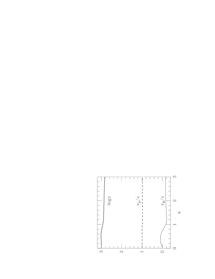
Figure 5:

References

- (1) Arons, J., 1981, ApJ, 248, 1099
- (2) Begelman, M, 1998, ApJ, 493, 291
- (3) Bogovalov, S. V., 1997, A& A, 327, 662
- (4) Camenzind, M., 1986, A& A, 162, 32
- (5) Cheng, K. J., Ho, C. & Ruderman, M., 1986, ApJ, 300, 500
- (6) Contopoulos, J., 1994, ApJ, 432, 508
- (7) Contopoulos, J., 1995, ApJ, 446, 67
- (8) Daugherty, J. K. & Harding, A. K., 1982, ApJ, 252, 337
- (9) Fendt, C., Camenzind, M. & Appl, S., 1995, A& A, 300, 791
- (10) Goldreich, P. & Julian, W. H., 1969, ApJ, 157, 869
- (11) Harding, A. K., 1981, ApJ, 245, 267
- (12) Kennel, C. F. & Coroniti, F. V., 1984, ApJ, 283, 694
- (13) Li, Z-Y, Chiueh, T. & Begelman, M. C., 1992, ApJ, 394, 459
- (14) Li, J. & Melrose, D. B., 1994, MNRAS, 270, 687
- (15) Mestel, L & Pryce, M. H. L., 1992, MNRAS, 254, 355
- (16) Mestel, L & Shibata, S., 1994, MNRAS, 271, 621
- (17) Michel, F. C., 1973a, ApJL, 180, L133
- (18) Michel, F. C., 1973b, ApJ, 180, 207
- (19) Michel, F. C., 1982, Rev. Mod. Phys., 54, 1
- (20) Michel, F. C., 1991, Theory of Neutron Star Magnetospheres (University of Chicago Press: Chicago)
- (21) Press, W. H., Flannery, B. P., Teukolsky, S. A. & Vetterling, W. T., 1988, Numerical Recipes (Cambridge Univ. Pree: Cambridge)
- (22) Romani, R. W., 1996, ApJ, 470, 469
- (23) Scharleman, E. T. & Wagoner, R. V., 1973, ApJ, 182, 951
- (24) Shibata, S., 1991, ApJ, 378, 239
- (25) Shibata, S., 1995, MNRAS, 276, 537
- (26) Sulkanen, M. E. & Lovelace, R. V. E., 1990, ApJ, 350, 732