An Approximation to the Likelihood Function for Band–Power Estimates of CMB Anisotropies

Abstract

Band–power estimates of cosmic microwave background fluctuations are now routinely used to place constraints on cosmological parameters. For this to be done in a rigorous fashion, the full likelihood function of band–power estimates must be employed. Even for Gaussian theories, this likelihood function is not itself Gaussian, for the simple reason that band–powers measure the variance of the random sky fluctuations. In the context of Gaussian sky fluctuations, we use an ideal situation to motivate a general form for the full likelihood function from a given experiment. This form contains only two free parameters, which can be determined if the 68% and 95% confidence intervals of the true likelihood function are known. The ansatz works remarkably well when compared to the complete likelihood function for a number of experiments. For application of this kind of approach, we suggest that in the future both 68% and 95% (and perhaps also the 99.7%) confidence intervals be given when reporting experimental results.

1 Introduction

Six years after their first detection by the COBE satellite (Smoot et al. 1992), it is now well appreciated that cosmic microwave background (CMB) temperature fluctuations contain rich information concerning virtually all the fundamental cosmological parameters of the Big Bang model (Bond et al. 1994; Knox 1995; Jungman et al. 1996). New observations from a variety of experiments, ground–based and balloon–borne, as well as the two planned satellite missions, MAP and Planck Surveyor, are and will be supplying a constant stream of ever more precise data over the next decade.

It is in fact already possible to extract interesting information from the existing data set, consisting of almost 20 different experimental results (Lineweaver et al. 1997; Bartlett et al. 1998a,b; Bond & Jaffe 1998; Efstathiou et al. 1998; Hancock et al. 1998; Lahav & Bridle 1998; Lineweaver & Barbosa 1998a,b; Lineweaver 1998; Webster et al. 1998; Lasenby et al. 1999). These experimental results are most often given in the literature as power estimates within a band defined over a restricted range of spherical harmonic orders. Our compilation, similar to those of Lineweaver et al. (1997) and Hancock et al. (1998), is shown in Figure 1 and may be accessed at our web site. The band is defined either directly by the observing strategy, or during the data analysis, e.g., the electronic differencing scheme introduced by Netterfield et al. (1997). This permits a concise representation of a set of observations, reducing a large number of pixel values to only a few band–power estimates, and for this reason the procedure has been referred to as “radical compression” (Bond et al. 1998). If the sky fluctuations are Gaussian, as predicted by inflationary models, then little or nothing has been lost by the reduction to band–powers (Tegmark 1997). This is extremely important, because the limiting factor in statistical analysis of the next generation of experiments, such as, e.g., BOOMERanG, MAXIMA, and Archeops, is calculation time. Working with a much smaller number of band–powers, instead of the original pixel values, will be essential for such large data sets. The question then becomes how to correctly treat the statistical problem of parameter constraints starting directly with band–power estimates.

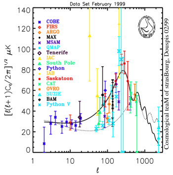
Figure 1: Present CMB power spectrum estimates. Flat band–powers are shown as a function of multipole order $l$. The data and references can be found at http://astro.u-strasbg.fr/Obs/COSMO/CMB/tabcmb.html. The solid curve is a flat CDM model with $\Omega=0.4$, $\Lambda=0.6$, $H_{o}=40$ km/s/Mpc, $Q=19\;\mu$K, $\Omega_{b}h^{2}=0.006$ and $n=0.94$, while the dotted line represents an open model with $\Omega=0.2$, $\Lambda=0$, $H_{o}=60$ km/s/Mpc, $Q=20\;\mu$K, $\Omega_{b}h^{2}=0.015$ and $n=1$ (no gravitational waves and no reionization).

Standard approaches to parameter determination, whether they be frequentist or Bayesian, begin with the construction of a likelihood function. For Gaussian fluctuations, the only kind we consider here, this is a multivariant Gaussian in the pixel temperature values, where the covariance matrix is a function of the model parameters (see below). The likelihood is then used as a function of the parameters, but as just mentioned, the large number of pixels makes this object very computationally cumbersome. It would be extremely useful to be able to define a likelihood function starting directly with the power estimates in Figure 1. This is the concern of this paper, where we develop an approximation to the the full likelihood function which requires only band–power estimates and very limited experimental details. As always in such procedures, it is worth emphasizing that the likelihood function, and therefore all derived constraints, only applies within the context of the particular model adopted. In our discussion, we shall focus primarily on inflationary scenarios, whose theoretical predictions have become easily calculable thanks to the development of fast Boltzmann codes, such as CMBFAST (Seljak & Zaldarriaga 1996; Zaldarriaga et al. 1998).

Much of the recent work on parameter determination has relied on the traditional $\chi^{2}$–fitting technique. As is well known, this amounts to a likelihood approach for observables with a Gaussian probability distribution. Band–power estimates do not fall into this category (Knox 1995; Bartlett et al. 1998c; Bond et al. 1998; Wandelt et al. 1998) – they are not Gaussian distributed variables, not even in the case of underlying Gaussian temperature fluctuations. The reason is clear: power estimates represent the variance of Gaussian distributed pixel values (the sky temperature fluctuations), and they therefore have a distribution more closely related to the $\chi^{2}$–distribution.

We begin, in the following section, by a general discussion of the likelihood approach applied to CMB observations. In the context of an ideally simple situation, we find the exact analytic form for the likelihood function of a band–power estimate. Reflections concerning the likelihood function in the context defined by actual experiments motivates us to propose this analytic form as an approximation, or ansatz, in the more general case. It is extremely easy to use, requiring little information in order to be applied to an experimental setup, because it contains only two adjustable parameters. These can be completely determined if one is given two confidence intervals, say the 68% and 95% confidence intervals, of the true, underlying likelihood distribution (notice that here we see the non–Gaussian nature of the likelihood – a Gaussian function would only require one confidence interval, besides the best power estimate, to be completely determined). We ask that in the future at least two confidence intervals be given when reporting experimental band–power estimates (more would be better, say for adjusting more complicated functional forms). An important limitation of the approach is the inability at present to account for more than one, correlated band–powers, as will be discussed further below.

We quantitatively test the accuracy of the approximation in Section 3 by comparison to several experiments for which we have calculated the full likelihood function. The approximation works remarkably well, and it can represent a substantial improvement over both single and “2–winged” Gaussian forms commonly used in standard $\chi^{2}$–analyses; and it is as easy to use as the latter. The proposed likelihood approximation, the main result of this paper, is given in Eqs. (18) – (20). We plan to maintain a web page with a table of the best fit parameters required for its use. Detailed application of the approximate likelihood function to parameter constraints and to tests of the Gaussianity of the observed fluctuations is left to future papers. Other, similar work has been performed by Bond et al. (1998) and Wandelt et al. (1998).

2 Likelihood Method

2.1 Generalities

Temperature anisotropies are described by a 2–dimensional random field $\Delta(\hat{n})\equiv(\delta T/T)(\hat{n})$, where $\hat{n}$ is a unit vector on the sphere. This means we imagine that the temperature at each point has been randomly selected from an underlying probability distribution, characteristic of the mechanism generating the perturbations (e.g., Inflation). It is convenient to expand the field in spherical harmonics:

$$\Delta(\hat{n})=\sum_{lm}a_{lm}Y_{lm}(\hat{n})$$ (1)

For Inflation generated perturbations, the coefficients $a_{lm}$ are Gaussian random variables with zero mean – $<a_{lm}>_{ens}=0$ – and covariance

$$<a_{lm}a^{*}_{l^{\prime}m^{\prime}}>_{ens}=C_{l}\delta_{ll^{\prime}}\delta_{mm^{\prime}}$$ (2)

This latter equation defines the power spectrum as the set of $C_{l}$. The indicated averages are to be taken over the theoretical ensemble of all possible anisotropy fields, of which our observed CMB sky is but one realization. Since the harmonic coefficients are Gaussian variables and the expansion is linear, it is clear that the temperature values on the sky are also Gaussian, and they therefore follow a multivariate Gaussian distribution (with an uncountably infinite number of variables, one for each position on the sky). The covariance of temperatures separated by an angle $\theta$ on the sky is given by the correlation function

$$C(\theta)\equiv<\Delta(\hat{n}_{1})\Delta(\hat{n}_{2})>_{ens}=\frac{1}{4\pi}\sum_{l}(2l+1)C_{l}P_{l}(\mu)$$ (3)

where $P_{l}$ is the Legendre polynomial of order $l$ and $\mu=\cos\theta=\hat{n}_{1}\cdot\hat{n}_{2}$. The form of this equation, which follows directly from Eq. (2), is dictated by the statistical isotropy of the perturbations – the two–point correlation function can only depend on separation.

Observationally, one works with sky brightness integrated over the experimental beam

$$\Delta_{b}(\hat{n}_{p})=\int\;d\Omega\Delta(\hat{n})B(\hat{n}_{p},\hat{n})$$ (4)

where $B$ is the beam profile and $\hat{n}_{p}$ gives the position of the beam axis. The beam profile may or may not be a sole function of $\hat{n}_{p}\cdot\hat{n}$, i.e., of the separation between sky point and beam axis; if it is, then this equation is a simple convolution on the sphere, and we may write

$$C_{b}(\theta)\equiv<\Delta_{b}(\hat{n}_{1})\Delta_{b}(\hat{n}_{2})>_{ens} = \frac{1}{4\pi}\sum_{l}(2l+1)C_{l}$$

$$\hskip 28.45274pt\times|B_{l}|^{2}P_{l}(\mu)$$

for the beam–smeared correlation function, or covariance between experimental beams separated by $\theta$. The beam harmonic coefficients, $B_{l}$, are defined by

$$B(\theta^{\prime})=\frac{1}{4\pi}\sum_{l}(2l+1)B_{l}P_{l}(\mu^{\prime})$$ (6)

with $\hat{n}_{p}\cdot\hat{n}=\cos\theta^{\prime}=\mu^{\prime}$. For example, for a Gaussian beam, $B(\theta)=1/(2\pi\sigma^{2})e^{-\theta^{2}/2\sigma^{2}}$ and $B_{l}=e^{-l(l+1)\sigma^{2}/2}$.

Given these relations and a CMB map, it is now straightforward to construct the likelihood function, whose role is to relate the $N_{\rm pix}$ observed sky temperatures, which we arrange in a data vector with elements $d_{i}\equiv\Delta_{b}(\hat{n}_{i})$, to the model parameters, represented by a parameter vector $\overrightarrow{\Theta}$. As advertised, for Gaussian fluctuations (with Gaussian noise) this is simply a multivariate Gaussian:

$${\cal L}(\overrightarrow{\Theta})\equiv{\rm Prob}(\overrightarrow{d}|\overrightarrow{\Theta})=\frac{1}{(2\pi)^{N_{\rm pix}/2}|\@vec{C}|^{1/2}}e^{-\frac{1}{2}\overrightarrow{d}^{t}\cdot\@vec{C}^{-1}\cdot\overrightarrow{d}}$$ (7)

The first equality reminds us that the likelihood function is the probability of obtaining the data vector given the model as defined by its set of parameters. In this expression, $\@vec{C}$ is the pixel covariance matrix:

$$C_{ij}\equiv<d_{i}d_{j}>_{ens}=T_{ij}+N_{ij}$$ (8)

where the expectation value is understood to be over the theoretical ensemble of all possible universes realisable with the same parameter vector. The second equality separates the model’s pixel covariance, $\@vec{T}$, from the noise induced covariance, $\@vec{N}$. According to Eq. (2.1), $T_{ij}=C_{b}(\theta_{ij})$. The parameters may be either the individual $C_{l}$ (or band–powers, discussed below), or the fundamental cosmological constants, $\Omega,H_{o}$, etc… In the former case, Eq. (2.1) shows how the parameters enter the likelihood; in the latter situation, the parameter dependence enters through detailed relations of the kind $C_{l}[\overrightarrow{\Theta}]$, specified by the adopted model (e.g., Inflation). Notice that if one only desires to determine the $C_{l}$, then only the assumption of Gaussianity is required.

Many experiments report temperature differences; and even if the starting point is a true map, one may wish to subject it to a linear transformation in order to define bands in $l$–space over which power estimates are to be given. Thus, it is useful to generalize our approach to arbitrary homogeneous, linear data combinations, represented by a transformation matrix $\@vec{A}$: $\overrightarrow{d}^{\prime}=\@vec{A}\cdot\overrightarrow{d}$. Since the transformation is linear, the new data vector retains a multivariate Gaussian distribution (with zero mean), but with a modified covariance matrix: $\@vec{C}^{\prime}=\@vec{A}\cdot\@vec{C}\cdot\@vec{A}^{t}$. As a consequence, the transformed pixels, $\overrightarrow{d}^{\prime}$, may be treated in the same manner as the originals, and so we will hereafter use the term generalized pixels to refer to the elements of a general data vector which may be either real sky pixels or some transformed version thereof. The elements of the new theory covariance matrix are (using the summation convention)

$$T^{\prime}_{ij}=A_{im}A_{jn}T_{mn}=\frac{1}{4\pi}\sum_{l}(2l+1)C_{l}W_{ij}(l)$$ (9)

where $W_{ij}(l)\equiv A_{im}A_{jn}P_{l}(\mu_{mn})|B_{l}|^{2}$. The window function is usually defined as $W_{ii}(l)$, i.e., the diagonal elements of a more general matrix $\@vec{W}(l)$. Normally, one tries to find a transformation which leads to a strongly diagonal $\@vec{W}(l)$ and diagonal noise matrix (see comment below).

An example is helpful. Consider a simple, single difference $\Delta_{diff}\equiv\Delta_{b}(\hat{n}_{1})-\Delta_{b}(\hat{n}_{2})$, whose variance is given by $<\Delta_{diff}^{2}>_{ens}=2[C_{b}(0)-C_{b}(\theta)]$. This may be written in terms of multipoles as

$$<\Delta_{diff}^{2}>=\frac{1}{4\pi}\sum_{l}(2l+1)C_{l}\left\{2|B_{l}|^{2}\left[1-P_{l}(\mu)\right]\right\}$$ (10)

identifying the diagonal elements of $\@vec{W}$ as the expression in curly brackets. Notice that the power in this variance is localized in $l$–space, being bounded towards large $l$ by the beam smearing and towards small $l$ by the difference. The off–diagonal elements of $\@vec{C}$ depend on the relative positions and orientations of the differences on the sky; in general these elements are not expressible as simple Legendre series.

Band–powers are defined via Eq. (9). One reduces the set of $C_{l}$ contained within the window to a single number by adopting a spectral form. The so–called flat band–power, $\delta T_{\rm fb}$, is established by using $C_{l}\equiv 2\pi(\delta T_{\rm fb})^{2}/[l(l+1)]$, leading to

$$\@vec{T}=\frac{1}{2}\delta T_{\rm fb}^{2}\sum_{l}\frac{(2l+1)}{l(l+1)}\@vec{W}(l)$$ (11)

In this fashion, we may write Eq. (7) in terms of the band–power and treat the latter as a parameter to be estimated. This then becomes the band–power likelihood function, ${\cal L}(\delta T_{\rm fb})$. One obtains the points shown in Figure 1 by maximizing this likelihood function; the errors are typically found by in a Bayesian manner, by integration over ${\cal L}$ with a uniform prior. Notice that the variance due to the finite sample size (i.e., the sample variance, but also known as cosmic variance when one has full sky coverage) is fully incorporated into the analysis – the likelihood function “knows” how many pixels there are.

An important remark at this stage concerns the construction of Figure 1. We see here that this figure is only valid for Gaussian perturbations, because it relies on Eq. (7), which assumes Gaussianity at the outset. If the sky fluctuations are non–Gaussian, then these estimates must all be re–evaluated based on the true nature of the sky fluctuations, i.e., the likelihood function in Eq. (7) must be redefined. The same comment applies to any experiment which has an important non–Gaussian noise component – the likelihood function must incorporate this aspect in order to properly yield the power estimate and associated error bars.

What is the raison d’être for these band powers? The likelihood function is clearly greatly simplified if we can find a transformation $\@vec{A}$ which diagonalizes $\@vec{C}$ (signal plus noise). This can be done for a given model, but because $\@vec{C}$ depends on the model parameters, there is in general no unique such transformation valid for all parameter values. The one exception is for an ideal experiment (no noise, or uniform, uncorrelated noise) with full–sky coverage – in this case the spherical harmonic transformation is guaranteed, by Eq. (2), to diagonalize $\@vec{C}$ for any and all values of the model parameters. This linear transformation is represented by a matrix $A_{ij}\equiv Y_{i}(\hat{n}_{j})$, where $i=l^{2}+l+m+1$ is a unidimensional index for the pair $(l,m)$. It is the role of band–powers to approximately diagonalize the covariance matrix in more realistic situations, where sky coverage is always limited and noise is never uniform (and sometimes correlated), and in such a way as to concentrate the power estimates in as narrow bands as possible. Since this is not possible for arbitrary parameter values, in practice one adopts a fiducial model (particular values for the parameters) to define a transformation $\@vec{A}$ which compromises between the desires for narrow and independent bands (Bond 1995, Tegmark et al. 1997, Tegmark 1997, Bunn & White 1997).

2.2 Motivating an Ansatz

Given a set of band–powers, how should one proceed to constrain the fundamental cosmological parameters, denoted in this subsection by $\overrightarrow{\Theta}$? If we had an expression for ${\cal L}(\overrightarrow{\delta T_{\rm fb}})$, for our set of band–powers $\overrightarrow{\delta T_{\rm fb}}$, then we could write ${\cal L}(\overrightarrow{\delta T_{\rm fb}})=Prob(\overrightarrow{d}|\overrightarrow{\delta T_{\rm fb}})=Prob(\overrightarrow{d}|\overrightarrow{\delta T_{\rm fb}}[\overrightarrow{\Theta}])={\cal L}(\overrightarrow{\Theta})$. Thus, our problem is reduced to finding an expression for ${\cal L}(\overrightarrow{\delta T_{\rm fb}})$, but as we have seen, this is a complicated function of $\overrightarrow{\delta T_{\rm fb}}$, requiring use of all the measured pixel values and the full covariance matrix with noise – the very thing we are trying to avoid. Our task then is to find an approximation for ${\cal L}(\overrightarrow{\delta T_{\rm fb}})$. In order to better understand the general form expected for ${\cal L}(\overrightarrow{\delta T_{\rm fb}})$, we shall proceed by first considering a simple situation in which we may find an exact analytic expression for this function. We are guided by the observation that the covariance matrix may always be diagonalized around an adopted fiducial model. Although this remains strictly applicable only for this model, we imagine that the likelihood function could be approximated as a simple product of one–dimensional Gaussians near this point in parameter space. If we further suppose that the diagonal elements of the covariance matrix (its eigenvalues) are all identical, we can find a very manageable analytic expression for the likelihood in terms of the best power estimate. We will then pose this general form as an ansatz for more realistic situations, one which we shall test in the following section. We return to these remarks after developing the ansatz.

Consider, then, a situation in which the band temperatures (that is, generalized pixels which are the elements of the general data vector $\overrightarrow{d}^{\prime}$) are independent random variables ($\@vec{C}$ is diagonal) and that the experimental noise is spatially uncorrelated and uniform:

$$C_{ij}=(\sigma_{M}^{2}+\sigma_{N}^{2})\delta_{ij}$$ (12)

where $\sigma_{M}^{2}$ is the model–predicted variance and $\sigma_{N}^{2}$ is the constant noise variance. For simplicity, we assume that all diagonal elements of $\@vec{W}$ are the same, implying that $\sigma_{M}^{2}$ is a constant, independent of $i$. We discuss shortly the nature of such a data vector in actual observational set–ups. This situation is identical to one where $N_{\rm pix}$ values are randomly selected from a single parent distribution described by a Gaussian of zero mean and variance $\sigma_{M}^{2}+\sigma_{N}^{2}$. The band–power we wish to estimate is proportional to the model–predicted variance according to (i.e., Eq. 11)

$$\sigma_{M}^{2}=\delta T_{\rm fb}^{2}\times\frac{1}{2}\sum_{l}\frac{(2l+1)}{l(l+1)}W_{ii}(l)\equiv\delta T_{\rm fb}^{2}{\cal R}_{band}$$ (13)

(independent of $i$), and we know that in this situation the maximum likelihood estimator for the model–predicted variance is simply

$$[\hat{\sigma}_{M}]^{2}=\frac{1}{N_{\rm pix}}\sum_{i=1}^{N_{\rm pix}}d_{i}^{2}-\sigma_{N}^{2}\equiv[\hat{\delta T_{\rm fb}}]^{2}{\cal R}_{band}$$ (14)

as follows from maximizing the likelihood function

$${\cal L}(\sigma_{M})=\frac{1}{[2\pi(\sigma_{M}^{2}+\sigma_{N}^{2})]^{N_{\rm pix}/2}}e^{-\frac{N_{\rm pix}(\hat{\sigma}_{M}^{2}+\sigma_{N}^{2})}{2(\sigma_{M}^{2}+\sigma_{N}^{2})}}$$

Notice that this is a function of $\sigma_{M}$, which peaks at the best estimate $\hat{\sigma}_{M}$, and whose form is specified by the parameters $\hat{\sigma}_{M}$, $\sigma_{N}$ and $N_{\rm pix}$. To obtain the likelihood function for the band–power, we simply treat this as a function of $\delta T_{\rm fb}$, using Eq. (13), parameterized by $\hat{\delta T_{\rm fb}}$, $\sigma_{N}$ and $N_{\rm pix}$:

$${\cal L}(\delta T_{\rm fb}) = \frac{1}{[2\pi(\delta T_{\rm fb}^{2}{\cal R}_{band}+\sigma_{N}^{2})]^{N_{\rm pix}/2}}$$

$$\hskip 56.9055pt\times e^{-\frac{N_{\rm pix}(\hat{\delta T_{\rm fb}}^{2}{\cal R}_{band}+\sigma_{N}^{2})}{2(\delta T_{\rm fb}^{2}{\cal R}_{band}+\sigma_{N}^{2})}}$$

$$\equiv G(\delta T_{\rm fb};\hat{\delta T_{\rm fb}},\sigma_{N},N_{\rm pix})$$

It clearly peaks at $\hat{\delta T_{\rm fb}}$. Thus, in this ideal case, we have a simple band–power likelihood function, with corresponding best estimator, $\hat{\delta T_{\rm fb}}$, given by Eq. (14).

Although not immediately relevant to our present goals, it is all the same instructive to consider the distribution of $\hat{\delta T_{\rm fb}}$. This is most easily done by noting that the quantity

$$\chi^{2}_{N_{\rm pix}}\equiv\sum_{i=1}^{N_{\rm pix}}\frac{d_{i}^{2}}{\sigma_{M}^{2}+\sigma_{N}^{2}}$$ (16)

is $\chi^{2}$–distributed with $N_{\rm pix}$ degrees of freedom. We may express the maximum likelihood estimator for the band–power in terms of this quantity as

$$\hat{\delta T_{\rm fb}}^{2}={\cal R}_{band}^{-1}\left[\frac{(\sigma_{M}^{2}+\sigma_{N}^{2})}{N_{\rm pix}}\chi^{2}_{N_{\rm pix}}-\sigma_{N}^{2}\right]$$ (17)

From $<\chi^{2}_{N_{\rm pix}}>=N_{\rm pix}$, we see immediately that the estimator is unbiased

$$<\hat{\delta T_{\rm fb}}^{2}>_{ens}={\cal R}_{band}^{-1}\sigma_{M}^{2}=\delta T_{\rm fb}^{2}$$

Its variance is

$$Var(\hat{\delta T_{\rm fb}}^{2}) = {\cal R}_{band}^{-2}\frac{(\sigma_{M}^{2}+\sigma_{N}^{2})^{2}}{N_{\rm pix}^{2}}Var(\chi^{2}_{N_{\rm pix}})$$

$$= 2{\cal R}_{band}^{-2}(\sigma_{M}^{2}+\sigma_{N}^{2})^{2}/N_{\rm pix}$$

explicitly demonstrating the influence of sample/cosmic variance (related to $N_{\rm pix}$).

All the above relations are exact for the adopted situation – Eq. (2.2) is the complete likelihood function for the band–power defined by the generalized pixels satisfying Eq. (12). Such a situation could be practically realized on the sky by observing well separated generalized pixels to the same noise level; for example, a set of double differences scattered about the sky, all with the same signal–to–noise. This is rarely the case, however, as scanning strategies must be concentrated within a relatively small area of sky (one makes maps!). This creates important off–diagonal elements in the theory covariance matrix $\@vec{T}$, representing correlations between nearby pixels due to long wavelength perturbation modes. In addition, the noise level is quite often not uniform and sometimes even correlated, adding off–diagonal elements to the noise covariance matrix. Thus, the simple form proposed in Eq. (12) is never achieved in actual observations. Nevertheless, as mentioned, even in this case one could adopt a fiducial theoretical model and find a transformation $\@vec{A}$ which diagonalizes the full covariance matrix $\@vec{C}$, thereby regaining one important simplifying property of the above ideal situation. The diagonal elements of the matrix are then its eigenvalues. Because of the correlations in the original matrix, we expect there to be fewer significant eigenvalues than generalized pixels; this will be relevant shortly. One could then work with a reduced matrix consisting of only the significant eigenvalues, an approach reminiscent of the signal–to–noise eigenmodes proposed by Bond (1995), and also known as the Karhunen-Loeve transform (Bunn & White 1997, Tegmark et al. 1997). There remain two technical difficulties: the covariance matrix does not remain diagonal as we move away from the adopted fiducial model by varying $\delta T_{\rm fb}$ – only when this band–power corresponds to the fiducial model is the matrix really diagonal. The second complicating factor is that the eigenvalues are not identical, which greatly simplified the previous calculation.

All of this motivates us to examine the possibility that a likelihood function of the form (2.2) could be applied, with appropriate redefinitions of $N_{\rm pix}$ and $\sigma_{N}$. We therefore proceed by renaming these latter $\nu$ and $\beta$, respectively, and treating them as parameters to be adjusted to best fit the full likelihood function. Thus, given an actual band–power estimate, $\delta T_{\rm fb}^{(o)}$ (i.e., an experimental result), we propose $G(\delta T_{\rm fb};\delta T_{\rm fb}^{(o)},\beta,\nu)$ as an ansatz for the band–power likelihood function, with parameters $\nu$ and $\beta$:

$${\cal L}(\delta T_{\rm fb}) \propto X^{\nu/2}e^{-X/2}$$ (18)

$$X[\delta T_{\rm fb}] \equiv \frac{([\delta T_{\rm fb}^{(o)}]^{2}+\beta^{2})}{([\delta T_{\rm fb}]^{2}+\beta^{2})}\nu$$

We have only two parameters – $\nu$ and $\beta$ – to determine in order to apply the ansatz. This can be done if two confidence intervals of the complete likelihood function are known in advance. For example, suppose we were given both the 68% ($\sigma^{+}_{68}$ & $\sigma^{-}_{68}$) and 95% ($\sigma^{+}_{95}$ & $\sigma^{-}_{95}$) confidence intervals; then we could fix the two parameters with the equations

$$0.68 = \frac{\int_{\delta T_{\rm fb}^{(o)}-\sigma^{-}_{68}}^{\delta T_{\rm fb}^{(o)}+\sigma^{+}_{68}}d[\delta T_{\rm fb}]\;{\cal L}(\delta T_{\rm fb})}{\int_{0}^{\infty}d[\delta T_{\rm fb}]\;{\cal L}(\delta T_{\rm fb})}$$ (19)

$$0.95 = \frac{\int_{\delta T_{\rm fb}^{(o)}-\sigma^{-}_{95}}^{\delta T_{\rm fb}^{(o)}+\sigma^{+}_{95}}d[\delta T_{\rm fb}]\;{\cal L}(\delta T_{\rm fb})}{\int_{0}^{\infty}d[\delta T_{\rm fb}]\;{\cal L}(\delta T_{\rm fb})}$$ (20)

We shall see in the next section (Figures 2–7) that this produces excellent approximations. This is the main result of this paper.

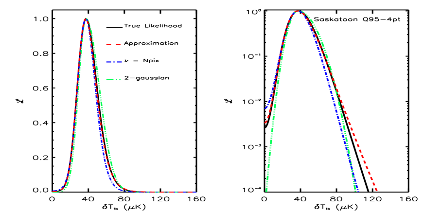
Figure 2: Comparison to the Saskatoon Q–band 1995 4–point difference. The value of the likelihood is plotted as a function of the band–power, $\delta T_{\rm fb}$, in both linear (left) and logrithmic (right) scales. The solid (black) curve in each case gives the true likelihood function, while the dashed (red) curve corresponds to the proposed approximation based on two confidence intervals. The dot–dashed (blue) curve is the ansatz with $\nu=N_{\rm pix}=24$ and $\beta$ adjusted to the 68% confidence interval (see text). A “2–winged Gaussian” with different positive–going and negative-going errors is shown as the three–dotted–dashed (green) curve. All curves have been normalized to unity at their peaks.

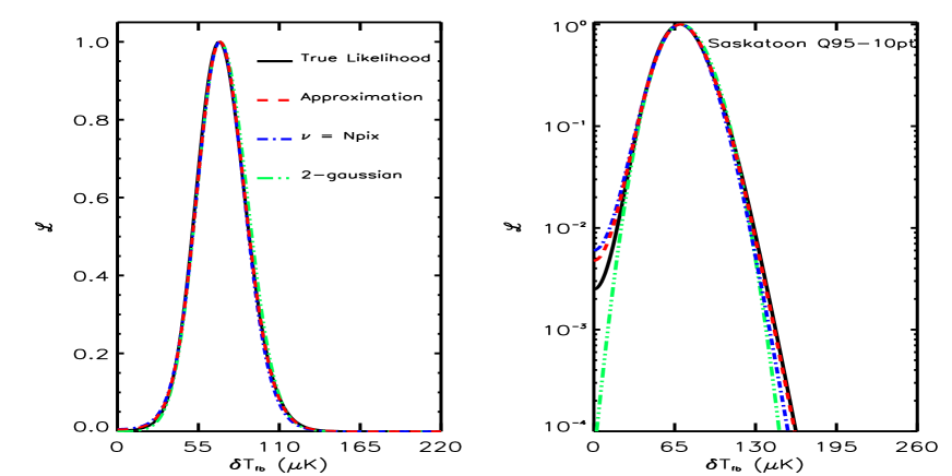
Figure 3: Comparison to the Saskatoon Q–band 1995 10–point difference. The line-styles are the same as in the previous figure; here $N_{\rm pix}=48$ for the dot–dashed (blue) line.

Unfortunately, most of the time only the 68% confidence interval is reported along with an experimental result (we hope that in the future authors will in fact supply at least two confidence intervals). Is there any way to proceed in this case? For example, one could try to judiciously choose $\nu$ and then adjust $\beta$ with Eq. (19). The most obvious choice for $\nu$ would be $\nu=N_{\rm pix}$, although from our previous discussion, we expect this to be an upper limit to the number of significant degrees–of–freedom (the significant eigenvalues of $\@vec{C}$), due to correlations between pixels. The comparisons we are about to make in the following section show that a smaller number of effective pixels (i.e., value for $\nu$) is in fact required for a good fit to the true likelihood function. One could try other games, such as setting $\nu\equiv$ (scan length)/(beam FWHM) for unidimensional scans. This also seems reasonable, and certainly this number is less than or equal to the actual number of pixels in the data set, but we have found that this does not always work satisfactorily. The availability of a second confidence interval permits both parameters, $\nu$ and $\beta$, to be unambiguously determined and in such a way as to provide the best possible approximation with the proposed ansatz.

Bond et al. (1998) have recently examined the nature of the likelihood function and discussed two possible approximations. The form of the ansatz just presented is in fact identical to one of their proposed approximations, parameterized by $x$ and $G$. These parameters are simply related to our $\nu$ and $\beta$ as follows: $x=\beta^{2}$ and $G=\nu$.

Notice that the above development and motivation for the ansatz essentially follow for a single band–power. A set of uncorrelated power estimates is then easily treated by simple multiplication. However, the approximation as proposed does not simultaneously account for several correlated band–powers, and it’s accuracy is therefore limited by the extent to which such inter–band correlations are important in a given data set. As a further remark along these lines, we have noted that flat–band estimates of any kind, be it from a complete likelihood analysis or not, do not always contain all relevant experimental information, (Douspis et al. 2000); any method based on their use is then fundamentally limited by nature of the lost information.

The only way to test the ansatz is, of course, by direct comparison to the full likelihood function calculated for a number of experiments. If it appears to work for a few such cases, then we may hope that it’s general application is justified. We now turn to this issue.

3 Testing the approximation

In order to quantitatively test the proposed ansatz, we have calculated the complete likelihood function for several experiments. Our aim will be to compare the true likelihoods to the approximation. Figures 2–5 summarize our comparisons with the Saskatoon and MAX data sets. For the Saskatoon and MAX experiments, we compare the approximation directly to the band–power likelihood functions. In all cases, the complete likelihood functions have been calculated as outlined in Section 2 above.

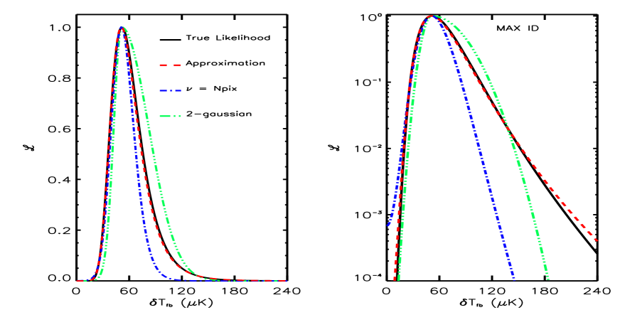
Figure 4: Comparison to the MAX ID likelihood function. This is the combined likelihood for the 3 frequency channels, 3.5, 6 and 9 $cm^{-1}$. Linestyles are the same as in the previous two figures, and here $N_{\rm pix}=21$ applies to the dot–dashed (blue) line.

The first comparison will be made to the Saskatoon Q–band 1995 4–point and 10–point differences (experimental information can be found in Netterfield et al. 1997; all relevant information concerning the experiment can be found on the group’s web page ; for useful and detailed information on a number of experiments, see Caltech’s web page). This particular choice of window functions was arbitrary. The approximation, applied using the constraints (19) and (20), is shown in Figures 2 and 3 as the dashed (red) curve. We see that it provides a good representation of the complete likelihood functions, traced by the solid (black) curves in each figure; in fact, the fit is truly spectacular for the 10–point difference. Taking as a benchmark the rule–of–thumb that 1, 2 and 3 $\sigma$ confidence intervals may be estimated by $2\Delta\ln{\cal L}=1$, 4 and 9, respectively, we see that the approximation reproduces almost perfectly all of these, and more.

Consider now setting $\nu=N_{\rm pix}=24$ and $48$, for the 4–point and 10–point differences, respectively, and then adjusting $\beta$ to the 68% confidence interval. In so doing, we obtain the dot–dashed (blue) curves, which in fact are not too bad in both cases. These values of $N_{\rm pix}$ should be compared to the values of $\nu=16$ and $41$ found previously by adjusting to two confidence intervals. Thus, we see that the effective number of degrees–of–freedom describing these Saskatoon likelihood functions is indeed $\nu\leq N_{\rm pix}$, as we expected from the above discussion.

Finally, the 3–dot–dashed (green) curves show “2–winged” Gaussians with separate positive– and negative– going variances, sometimes employed in traditional $\chi^{2}$–analyses. This is also a fare representation of the two likelihood functions, although the proposed ansatz does perform slightly better. We will return to this point, but we should not be too surprised that the Gaussian works reasonably well when, as here, $\nu$ becomes large (all the same, notice that the curves are not symmetric and that a single Gaussian, with a single $\sigma$, would not fare particularly well).

Comparison to the MAX experiment is shown in Figure 4 for the region ID (experimental details can be found in Tanaka et al. 1996); we have combined all three frequency channels to construct the complete likelihood function. The scan strategy consisted in taking $N_{\rm pix}=21$ single differences aligned along a unidimensional scan. Once again, the approximation, applied using Eqs. (19) and (20), supplies an excellent representation of the likelihood function, down to values well below “$3\sigma$” (0.01 of the peak). The effective number of degrees–of–freedom is $\nu=8.5$, demonstrating again that $\nu\leq N_{\rm pix}$. Here, the difference is rather large, due to the significant overlap between adjacent pixels along the scan, and we see that the ansatz with $\nu=N_{\rm pix}$ does not produce a good approximation.

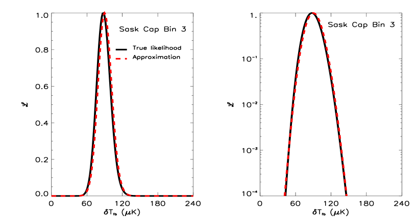
Figure 5: Comparison to a Saskatoon bin consisting of the 10–, 11– and 12–point differences (bands) from the K–band 1994, Q–band 1994 and Q-band 1995 CAP data. As previously, the solid black line shows the true likelihood function, while the dashed (red) curve displays the approximation based on two confidence intervals. This Figure demonstrates that the approximation works well even when several individual bands are combined to form a band–power likelihood.

Could there a way to proceed if only one confidence interval is given? This would require a choice for one of the parameters, say $\nu$, based on some knowledge of the scan strategy. We have just seen that for MAX $\nu=N_{\rm pix}$ leads to a bad representation of the likelihood function. One might be tempted to try instead $\nu=$ (scan length)/(beam FWHM)$=8.8$ , which is in fact very close to the best value of $\nu$ found from adjusting to two confidence intervals. Although this is successful in this case, it is nevertheless guess–work, the problem being that it is really not clear if there is a unique rule for judiciously choosing $\nu$. For Saskatoon, $\nu=N_{\rm pix}$ worked reasonably well, while here it does not, something much less being required because of the significant redundancy in the scan. We have found that it is difficult to justify a priori a general rule for choosing $\nu$ when lacking two confidence intervals. The most sure way of finding the effective number of degrees–of–freedom to be used in the ansatz remains the use of two confidence intervals,  via Eqs. (19) and (20).

A noteworthy aspect of this MAX likelihood function is its asymmetry, i.e., it is manifestly non–Gaussian. Even a “2–winged” Gaussian is clearly a very bad representation. As the number of statistically independent elements entering the power estimation increases, we should expect the likelihood function to approach a Gaussian distribution. The question is, what is meant by statistically independent elements? It is obviously not something like $2l+1$, for MAX covers multipoles near 100; rather, as we have argued above, it is really the parameter $\nu$ which measures this, what we have been calling the effective number of degrees–of–freedom. The fact that $\nu\leq N_{\rm pix}$ tells us that the number of generalized pixels is an upper limit to this number degrees–of–freedom determining the non–Gaussian nature of the likelihood function. We make the connection to the familiar $2l+1$–rule only when we have full–sky coverage and bands consisting of single multipoles; then, the number of generalized pixels defining each (single multipole) band corresponds to $2l+1$. In the general case, it is more useful and correct to reason with the number of pixels (really, $\nu$). We may also conclude from this that although experiments with relatively large sky coverage should provide Gaussian likelihood functions on scales much smaller than the survey area, band–power estimates on scales approaching the survey area will always be non–Gaussian. The proposed ansatz represents a substantial improvement over either a single or “2–winged” Gaussian in such cases.

These comparisons focus on simple cases where the power over a single band defined by the observing strategy is to be estimated, although in the MAX case the analysis did include three frequency channels simultaneously. A more subtle test of the approximation is its extension to a power estimate over several bands defined by different window functions. Such is the situation presented by the five standard Saskatoon power bins. Each bin comprises several bands, of the type considered above, and the bin power is estimated using the joint likelihood of the contributing bands, including all band–band correlations. One could worry that the information carried by several bands might not be adequately incorporated by the two parameters of the ansatz.

In Figure 5 we compare the approximation to the likelihood function of a combination of 10–, 11– and 12–point differences. Included are the K–band 1994 and Q–band 1994 and 1995 CAP data. The true likelihood function for this bin is calculated from the complete covariance matrix accounting for all correlations, and the approximation was fit using two confidence intervals. Even in this more complicated situation we see that the ansatz continues to work quite well, once the appropriate best power estimate and errors for the complete bin are used to find $\nu$ and $\beta$.

It is on the basis of such comparisons that we believe the proposed ansatz and method of application produces acceptable likelihood functions. Besides the comparisons shown here, we have also tested the approximation against 11 other complete likelihood functions, all kindly provided by K. Ganga; these comparisons may be viewed on our web page. The approximation works well in all cases. We emphasize again that the particular value of the proposed ansatz resides in its simplicity – we obtain very good approximations with little effort.

4 Conclusion

Study of CMB temperature fluctuations have over the short interval of time since their discovery become the cosmological tool with the greatest potential for determining the values of the fundamental cosmological constants. The present data set is already capable of eliminating some regions of parameter space, and this is only a fore-taste of what is to come. Experimental results are often quoted as band–power estimates, and for Gaussian sky fluctuations, these represent a complete description of an observation. Because there are far fewer band–powers than pixel values for any given experiment, the reduction to band–powers has been called “radical compression” (Bond et al. 1998); and as the number of pixels explodes with the next instrument generations, this kind of compression will become increasingly important in any systematic analysis of parameter constraints.

For these reasons, it is extremely useful to develop statistical methods which take as their input power estimates. Since most standard methods use as a starting point the likelihood function, one would like to have a simple expression for this quantity given a power estimate – one that does not require manipulation of the entire observational pixel set. One difficulty is that even for Gaussian sky fluctuations, the band–power likelihood function is not Gaussian, most fundamentally because the power represents an estimate of the variance of the pixel values. For any fiducial model, the data covariance matrix can be diagonalized and the likelihood function near this point in parameter space expressed as a product of individual Gaussians in the data elements (this is strictly speaking only possible for the model in question). This consideration lead us to examine the ideal situation where the eigenvalues of $\@vec{C}$ were all identical, for which we can analytically find the exact form of the likelihood function in terms of the best power estimate. Using this as motivation, we have proposed the same functional form for band–power likelihood functions, Eq. (18), as an ansatz in more general cases. It contains two free parameters, $\nu$ and $\beta$, which may be uniquely determined if two confidence intervals of the full likelihood function (the thing one is trying to fit) are known; for example, the 68% and 95% confidence intervals (Eqs. 19 and 20). We have seen that the resulting approximate distributions match remarkably well the complete likelihood functions for a number of experiments – those discussed here as well as 11 others (calculated by K. Ganga and B. Ratra). All of these comparisons may be viewed at our web site, where we also plan to provide and continually up–date the appropriate parameter values $\nu$ and $\beta$ for each published experiment.

Although at least one confidence interval is normally given in the literature (usually at 68%), a second confidence interval is rarely quoted. To aid the kind of approach proposed here, we would ask that in the future experimental band–power estimates be given with at least two likelihood–based confidence intervals (additional intervals, such as 99.8%, would allow one to fit other functional forms with 3 free parameters). This remains the surest way of finding the effective number of degrees–of–freedom of the likelihood, $\nu$. An otherwise a priori choice for this number appears difficult, among other things because it depends on the nature of the scan strategy. We have noted in this light that $\nu\leq N_{\rm pix}$, precisely because of correlations between pixels, which depend on the scan geometry.

One important aspect of the approximate nature of the proposed method is its inability to account for correlations between several band–powers. When analyzing a set of band–powers, one is obliged to simply multiply together their respective approximate likelihood functions. The accuracy of the approximation is thus limited by the extent to which inter–band correlations are important. Although one’s desire is to give experimental results as independent power estimates, this is not always possible. Furthermore, and as discussed in Douspis et al. (2000), the very use of flat–band powers may lead to a loss of relevant experimental information otherwise contained in the original pixel data. The accuracy of any method based on their use is thus additionally limited by the importance of this lost information. These limitations define in practice the approximate nature of the proposed method.

Another important point to make is that the approximation is extremely easy to use, as easy as the (inappropriate) $\chi^{2}$ method; and for experiments with a small number of significant degrees–of–freedom, it represents a substantial improvement over the latter. This is the case, for example, with the MAX ID likelihood function, and it will always be the case when estimating power on the largest scales of a survey. When the effective number of degrees–of–freedom becomes large, a Gaussian becomes an acceptable approximation, and the gain in using the proposed ansatz is less significant. Nevertheless, the approximation’s facile applicability promotes its use even in these cases. In the future, we will apply the proposed approximation in a systematic study of parameter constraints and for a test of the Gaussianity of the CMB fluctuations.

- (1) Bartlett J.G., Blanchard A., Le Dour M., Douspis M. & Barbosa D. 1998a, in: Fundamental Parameters in Cosmology (Moriond Proceedings), Eds. J. Trân Thanh Vân et al. (Editions Frontières: Paris, France), astro–ph/9804158
- (2) Bartlett J.G., Blanchard A., Douspis M. & Le Dour M. 1998b, to be published in: Evolution of Large–scale Structure: from Recombination to Garching (Munich, Germany), astro–ph/9810318
- (3) Bartlett J.G., Blanchard A., Douspis M. & Le Dour M. 1998c, to be published in: The CMB and the Planck Mission (Santander, Spain), astro–ph/9810316
- (4) Bond J.R., Jaffe A.H. & Knox L. 1998, astro–ph/9808264
- (5) Bond J.R. & Jaffe A.H. 1998, to appear in Philosophical Transactions of the Royal Society of London A, 1998. ”Discussion Meeting on Large Scale Structure in the Universe,” Royal Society, London, March 1998, astro–ph/9809043
- (6) Bond J.R. 1995, Phys. Rev. Lett. 74, 4369
- (7) Bond J.R., Crittenden R., Davis R.L., Efstathiou G. & Steinhardt P.J. 1994, Phys. Rev. Lett. 72, 13
- (8) Bunn E.F. & White M. 1997, ApJ 480, 6
- (9) Efstathiou G., Bridle S.L., Lasenby A.N., Hobson M.P. & Ellis R.S. 1998, astro–ph/9812226
- (10) Hancock S., Rocha G., Lasenby A.N. & Gutierrez C.M. 1998, MNRAS 294, L1
- (11) Jungman G., Kamionkowski M., Kosowsky A. & Spergel D. 1996, Phys. Rev. D54, 1332
- (12) Knox L. 1995, Phys. Rev. D52, 4307
- (13) Lahav O. & Bridle S.L. 1998, to be published in: Evolution of Large–scale Structure: from Recombination to Garching (Munich, Germany), astro–ph/9810169
- (14) Lasenby A.N., Bridle S.L. & Hobson M.P. 1999, to be published in: The CMB and the Planck Mission (Santander, Spain), astro–ph/9901303
- (15) Lineweaver C., Barbosa D., Blanchard A. & Bartlett J.G. 1997, A&A 322, 365
- (16) Lineweaver C.H. & Barbosa D. 1998a, A&A 329, 799
- (17) Lineweaver C.H. & Barbosa D. 1998b, ApJ 496, 624
- (18) Lineweaver C.H. 1998, ApJ 505, 69
- (19) Netterfield C.B., Devlin M.J., Jarolik N., Page L. & Wollack E.J. 1997, ApJ 474, 47
- (20) Seljak U. & Zaldarriaga M. 1996, ApJ469, 437
- (21) Smoot G.F., Bennett C.L., Kogut A. et al. 1992, ApJ 396, L1
- (22) Tanaka S.T., Clapp A.C., Devlin M.J. et al. 1996, ApJ 468, L81
- (23) Tegmark M., Taylor A.N. & Heavens A.F. 1997, ApJ 480, 22
- (24) Tegmark M. 1997, Phys Rev. D55, 5895
- (25) Wandelt B.D., Hivon E. & Górski K.M. 1998, astro–ph/9808292
- (26) Webster M., Bridle S.L., Hobson M.P., Lasenby A.N., Lahav O. & Rocha G. 1998, astro–ph/9802109
- (27) Zaldarriaga M., Seljak U. & Bertschinger E. 1998, ApJ 494, 491