Precise radial velocities of Proxima Centauri.

Abstract

We present differential radial velocity measurements of Proxima Centauri collected over 4 years with the ESO CES with a mean precision of $54\leavevmode\nobreak\ {\rm ms}^{-1}$. We find no evidence of a periodic signal that could corroborate the existence of a sub-stellar companion. We put upper limits (97% confidence) to the companion mass ranging from $1.1$ to $22\leavevmode\nobreak\ {\rm M}_{\rm Jup}$ at orbital periods of $0.75$ to $3000$ d, i.e. separations $0.008-2$ AU from Prox Cen. Our mass limits concur with limits found by precise astrometry (Benedict et al. 1998a and priv. comm.) which strongly constrain the period range $50-600$ d to $1.1-0.22\leavevmode\nobreak\ {\rm M}_{\rm Jup}$. Combining both results we exclude a brown dwarf or supermassive planet at separations $0.008-0.69$ AU from Prox Cen. We also find that, at the level of our precision, the RV data are not affected by stellar activity.

1 Introduction

Searches for companion objects to Proxima Centauri (Prox Cen, GJ551, V645 Cen, HIP70890), the nearest star ($d=1.2948\pm 0.041$ pc; M5Ve), date back 20 years to the astrometric work by Kamper & Wesselink (1978) and the infrared photometric scanning by Jameson et al. (1983). The most extensive search so far consists of astrometric monitoring with the HST FGS #3 (Benedict et al. 1998a) where an astrometric precision of $0.002^{\prime\prime}$ per axis and a detection limit for an astrometric variation of $0.001^{\prime\prime}$ was achieved, thereby strongly constraining the mass of a possible companion. Limits to the $K$-band magnitude of objects within projected separations of $1-10$ AU from Prox Cen were found by Leinert et al. (1997) to be $K=12.9-15.1$ mag, i.e. $\Delta K=3-5$ mag below the empirical end of the main-sequence.

Recently the efforts to detect substellar objects near Prox Cen culminated in the announcement of a possible companion by Schultz et al. (1998) who used the HST FOS as a coronographic camera. These authors reported excess light near Prox Cen seen in two images separated by 103 d. Within this time span, the suspected object appeared to have moved in separation from $0.23^{\prime\prime}$ to $0.34^{\prime\prime}$ (indicating a separation near $0.5$ AU) and in P.A. from $45^{\circ}$ to $100^{\circ}$. If interpreted as a companion the object would be $\approx 7$ mag fainter in the FOS red detector.

However, a subsequent observation with the HST WFPC2 at two epochs (separated by 21 d) by Golimowski & Schroeder (1998) could not verify the existence of any companion object to Prox Cen within a separation from $0.09^{\prime\prime}$ to $0.85^{\prime\prime}$ ($0.11-1.1$ AU). The authors concluded that they should have seen the object at only $\approx 3.7$ mag fainter than Prox Cen in their images taken at $1\mu$m. Consequently, they suggested that the excess light seen by Schultz et al. (1998) was an instrumental effect.

In this paper we report on 4 years of precise radial velocity (RV) monitoring of Prox Cen and contribute new evidence to the debate on a substellar companion.

2 The planet search program at the ESO CES

Our planet search program of 39 late-type stars using high-precision RVs was begun at ESO La Silla in Nov. 1992. Prox Cen was first observed in July 1993. We used the ESO 1.4m CAT telescope and CES spectrograph equipped with the f/4.7 Long Camera and ESO CCDs $\#30$ or $\#34$. The obtained resolving power, central wavelength and spectrum length were $100,000$, $5389$ Å, and $48$ Å. For high measurement precision for differential RVs we self-calibrated the spectrograph using an iodine ($I_{2}$) gas absorption cell temperature controlled at $50^{\circ}$ C (Kürster et al. 1994; Hatzes et al. 1996; Hatzes & Kürster 1994). To obtain RV measurements we model the stellar spectra as observed through the iodine cell using a ‘pure’ stellar spectrum (recorded without the iodine cell in the light path) and a ‘pure’ iodine ($I_{2}$) spectrum from dome flat measurements. The resulting RV data are then corrected to the solar system barycenter via the JPL ephemeris DE200.

For stars brighter than 5.5 mag our short-term (i.e. single night), best case long-term, and working long-term precisions (i.e. obtained under all observing conditions) are $4-7$, $11$, and $20-25\leavevmode\nobreak\ {\rm ms}^{-1}$, respectively (Kürster et al. 1994, 1998, 1999). Prox Cen is unique in our sample in that it is by far the faintest star we have observed ($V=11.01$ mag).

3 The RV measurements for Proxima Cen

Tab. 1 shows the journal of observations of our differential RV measurements. A total of 58 spectra from 29 nights were available. Before further analysis the spectra were combined into nightly bins (col. 1) as outlined below, with the bins containing between 1 and 5 spectra (col. 2).

While self-calibration with an iodine cell is an excellent method to overcome instrumental instabilities such as instrumental drifts other instabilities such as focus and alignment changes or instrument vibrations require (in principle) additional modelling of the instrumental profile (IP; Butler et al. 1996; Valenti et al. 1995). At low signal-to-noise (S/N) ratios such as obtained for Prox Cen IP reconstruction becomes impossible. However, to some extent one can overcome the remaining measurement uncertainty by modelling the observed spectra (star+iodine) with various combinations of pure star and iodine spectra.

Ten different pure star and pure iodine pairs (of the same night) were available to build models for each of the 58 star+iodine spectra. Based on goodness-of-fit some of the most inadequate models were rejected. Col. 3 gives the total number of the accepted star+iodine models for all the spectra in each nightly bin (sum over all spectra and models). For an intercomparison of the different models their RV zero points have to be matched. To do this we subtracted for each model the mean RV for the whole times series. Subsequently, we averaged for each star+iodine spectrum the RV data from the individual models. At last, nightly (bin) averages for the Julian day (col. 4) and RV data corrected to zero mean (col. 5) were calculated.

A first estimate of the RV error (col. 6) was then based on the rms scatter in each data bin together with a propagation of the error introduced by the process of matching the zero points for the different models. However, we found a positive correlation with a correlation coefficient of $+0.514$ between the total number of models in a bin (col. 3) and the error estimate (col. 6) meaning that these errors tend to be smaller when estimated from smaller numbers of models. This indicates that these error estimates are not representative of the true errors, in particular those from small numbers of models.

As an independent estimate of the weight of each data bin, col. 7 shows the combined S/N ratio per spectral pixel (mean values) of each data bin. We know from simulations (Hatzes & Cochran 1992) that the RV measurement error $\Delta RV\propto(S/N)^{-1}$ which serves to estimate the RV error. Choosing the constant of proportionality such that the mean of the resulting errors is equal to the total scatter in the RV measurements ($53.9\leavevmode\nobreak\ {\rm ms}^{-1}$) we obtain the equivalent RV errors listed in col. 8 of Tab. 1. Fig. 1 displays a time series of our RV data (29 bins) for Prox Cen with error bars corresponding to these equivalent errors.

Table 1: RV data for Prox Cen. Col. 1: bin number; col. 2: number of spectra in the bin; col. 3: total number of models for all spectra in the bin (i.e. the sum over all spectra and models); col. 4: mean Julian day of the bin; col. 5: mean differential RV of the bin; col. 6: rms scatter within the bin; col. 7: combined S/N ratio of the bin; col. 8: equivalent RV error as estimated from the S/N.

# # $\Sigma$	JD $-$	$\Delta$RV	rms	comb	erreq
Sp	$2,400,000$	$[$m/s$]$	$[$m/s$]$	S/N	$[$m/s$]$
1 1  7	49179.6643	$\leavevmode\nobreak\ 106.35$	$\leavevmode\nobreak\ 44.85$	21.46	71.78
2 2 14	49246.5034	$\leavevmode\nobreak\ -18.00$	$\leavevmode\nobreak\ 78.30$	17.88	86.16
3 2 18	49412.8484	$\leavevmode\nobreak\ \leavevmode\nobreak\ \leavevmode\nobreak\ 3.48$	$\leavevmode\nobreak\ 46.24$	23.87	64.54
4 4 34	49413.7676	$\leavevmode\nobreak\ -78.83$	$\leavevmode\nobreak\ 68.73$	34.10	45.18
5 5 40	49492.7022	$\leavevmode\nobreak\ \leavevmode\nobreak\ 52.55$	$\leavevmode\nobreak\ 85.96$	39.78	38.73
6 4 30	49548.5800	$\leavevmode\nobreak\ \leavevmode\nobreak\ 56.66$	$\leavevmode\nobreak\ 65.18$	35.12	43.86
7 2 15	49602.5149	$\leavevmode\nobreak\ \leavevmode\nobreak\ -2.23$	$\leavevmode\nobreak\ 60.60$	28.44	54.17
8 2 17	49794.7186	$\leavevmode\nobreak\ 107.13$	$103.27$	26.28	58.62
9 2 14	49795.6955	$\leavevmode\nobreak\ \leavevmode\nobreak\ 28.33$	$\leavevmode\nobreak\ 44.09$	28.10	54.82
10 2 16	49906.5524	$\leavevmode\nobreak\ \leavevmode\nobreak\ \leavevmode\nobreak\ 0.64$	$\leavevmode\nobreak\ 44.11$	27.91	55.20
11 1  9	49907.5940	$\leavevmode\nobreak\ \leavevmode\nobreak\ 60.47$	$\leavevmode\nobreak\ 38.37$	21.47	71.75
12 1  8	50146.7675	$\leavevmode\nobreak\ -70.90$	$\leavevmode\nobreak\ 42.87$	25.89	59.50
13 2 17	50229.6486	$\leavevmode\nobreak\ -40.73$	$\leavevmode\nobreak\ 56.75$	36.54	42.16
14 1  8	50230.6858	$\leavevmode\nobreak\ \leavevmode\nobreak\ 55.73$	$\leavevmode\nobreak\ 49.09$	26.82	57.44
15 2 14	50304.4963	$\leavevmode\nobreak\ \leavevmode\nobreak\ \leavevmode\nobreak\ 2.19$	$\leavevmode\nobreak\ 52.60$	30.92	49.82
16 2 15	50313.5397	$\leavevmode\nobreak\ -35.71$	$\leavevmode\nobreak\ 43.80$	40.39	38.14
17 2 14	50314.5965	$\leavevmode\nobreak\ -37.08$	$\leavevmode\nobreak\ 49.38$	37.62	40.95
18 2 13	50319.5519	$\leavevmode\nobreak\ -21.17$	$\leavevmode\nobreak\ 45.65$	31.42	49.03
19 1  6	50323.5606	$\leavevmode\nobreak\ -88.32$	$\leavevmode\nobreak\ 30.21$	25.87	59.55
20 1  7	50325.5852	$\leavevmode\nobreak\ -47.33$	$\leavevmode\nobreak\ 36.42$	27.10	56.85
21 2 17	50348.5179	$\leavevmode\nobreak\ \leavevmode\nobreak\ \leavevmode\nobreak\ 6.32$	$\leavevmode\nobreak\ 45.15$	38.82	39.68
22 2 18	50349.5142	$\leavevmode\nobreak\ -18.19$	$\leavevmode\nobreak\ 49.07$	36.90	41.75
23 1  7	50359.4920	$\leavevmode\nobreak\ -36.71$	$\leavevmode\nobreak\ 42.60$	24.56	62.72
24 2 17	50477.8459	$\leavevmode\nobreak\ \leavevmode\nobreak\ 45.31$	$\leavevmode\nobreak\ 73.70$	25.24	61.03
25 2 14	50478.8507	$-104.59$	$\leavevmode\nobreak\ 93.69$	21.67	71.09
26 2 18	50524.7935	$\leavevmode\nobreak\ \leavevmode\nobreak\ 43.71$	$\leavevmode\nobreak\ 48.86$	28.80	53.49
27 2 17	50551.6664	$\leavevmode\nobreak\ \leavevmode\nobreak\ 44.23$	$\leavevmode\nobreak\ 48.27$	28.03	54.96
28 2 12	50570.7647	$\leavevmode\nobreak\ \leavevmode\nobreak\ -3.27$	$\leavevmode\nobreak\ 61.04$	38.30	40.22
29 2 15	50648.5032	$\leavevmode\nobreak\ -10.02$	$\leavevmode\nobreak\ 42.17$	38.09	40.44

4 Period search

To look for a periodic signal that could manifest the presence of a companion, we searched the frequency range $f_{\rm min}=1/T\leavevmode\nobreak\ ...\leavevmode\nobreak\ f_{\rm max}=1/(2\Delta t)$, or $0.0007\leavevmode\nobreak\ ...\leavevmode\nobreak\ 0.5494\leavevmode\nobreak\ {\rm d}^{-1}$, where $T$ is the total time baseline and $\Delta t$ is the minimum separation between data points. Thus a period range of $1.8202\leavevmode\nobreak\ ...\leavevmode\nobreak\ 1428.6$ d was searched. The choice of the maximum frequency was made in analogy to the Nyquist criterion which, however, is well defined only for equidistant data sampling. Since most of our data sampling is much cruder than our minimum sampling any signals at periods shorter than about 5 d should be treated with care.

Figure 1: Time series of the differential RV data of Prox Cen.

Two different types of periodogram were used: a) the Scargle periodogram (Scargle 1982) which is equivalent to least squares sine fitting with equal weight for all data points; the power is proportional to the square of the amplitude of the corresponding sine wave; b) a sine-fitting routine that takes into account data errors by minimizing $\chi^{2}$; we used the equivalent errors (col. 8 of Tab. 1).

Fig. 2 shows only the Scargle periodogram, since the $\chi^{2}$ minimization approach yielded a very similar result that does not change the interpretation. ¿From 10,000 runs of a bootstrap randomization scheme (see Kürster et al. 1996; Murdoch et al. 1993) we determined the levels of the false alarm probability $\phi$ (FAP) corresponding to various power levels. As shown in Fig. 2 all periodogram peaks are insignificant having $\phi>90\%$.

In contrast to searching a period range signals at a priori known periods can be significant at smaller power levels $z$. For the Scargle periodogram the FAP is given by $\phi=1-(1-e^{-z})^{n}$, where $n$ is the number of independent frequencies in the search interval (Scargle 1982). Hence for a signal at a single a priori known period $\phi=e^{-z}$.

Periods that may be present are the period of the stellar rotation and that of the activity cycle. RV searches strongly benefit from ancilliary information such as the knowledge of these periods that aids the interpretation of RV data. Star spots and inhomogeneous granulation patterns in active stars cause distortions in stellar absorption lines; when sufficient resolution and/or signal-to-noise is lacking these distortions can be mis-interpreted as RV shifts that vary with the rotation period (rotational modulation) or with the activiy cycle. Estimates for the rotation period of Prox Cen were given by Benedict et al. (1998b; based on HST FGS photometry) finding $P_{\rm rot}=83.5$ d plus variability at the first harmonic, and by (Guinan & Morgan 1996; monitoring of the MgII h+k flux with IUE) who found $31.5\pm 1.5$ d. Benedict et al. (1998b) also estimate the length of Prox Cen’s activity cycle to be $\approx 1100$ d.

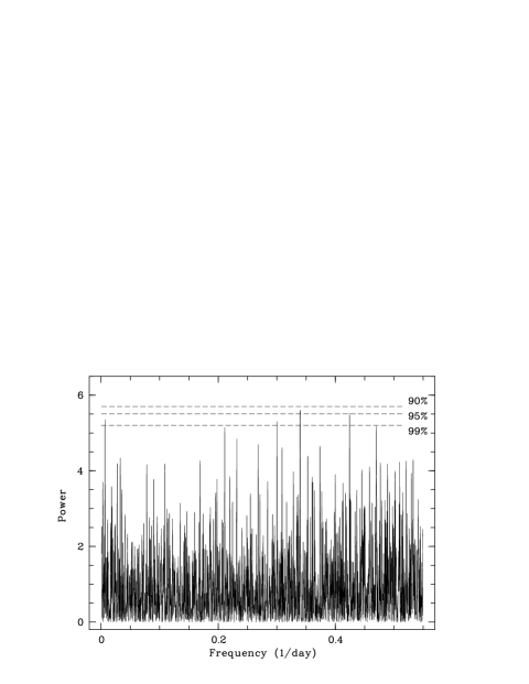
Figure 2: Periodogram for the RV data. Horizontal dashed lines correspond to various levels of the false alarm probability.

We do not find significant FAPs at any one of these periods nor at first harmonics or periods twice as large (relevant in case the literature values are first harmonics themselves). Allowing for some uncertainty in these period values we also searched their vicinities finding $\phi=0.47\%\leavevmode\nobreak\ (0.16\%)$ for $P=150.4\leavevmode\nobreak\ d$ and $\phi=1.32\%\leavevmode\nobreak\ (0.92\%)$ for $P=30.4\leavevmode\nobreak\ d$, where theoretical values, $\phi=e^{-z}$, as well as values bootstrapped from 10,000 runs (values in brackets) are given. At best, i.e. only if one allows for considerable errors in the original period estimates, a marginal detection of (1) a period twice as long as the rotation period by Benedict et al. (1998b) and (2) the rotation period by (Guinan & Morgan 1996) might be indicated.

Reconfiguration of active regions causes amplitude and phase changes in rotationally modulated signals complicating their detection in data that extend over many rotation cycles. However, our results concur with the findings by Saar et al. (1998) that predict an activity-related RV scatter of $<10\leavevmode\nobreak\ {\rm ms}^{-1}$ for rotation periods $>16$ d. It appears that the RV variation seen for Prox Cen is representative of our measurement precision for this faint star, and cannot be attributed to instrinsic stellar variability.

5 Limits to companion parameters

Lacking a clear RV signal in our Prox Cen data we used a Monte Carlo simulation to derive upper limits to the mass of still possible companions in the period range $0.75-3000$ d. Random data sets with the same temporal sampling and with the rms scatter of our data were created. We added sinusoidal signals with different periods, amplitudes, and phases, and evaluated their periodograms. At each period the amplitude was determined for which 99% of the periodograms showed a power corresponding to $\geq 1\%$ FAP. Hence the combined confidence for the detection of a sinusoidal signal is 98%. For eccentric orbits it may be somewhat lower.

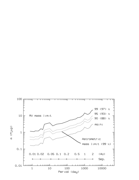
Figure 3: RV derived upper limits to the mass of companions to Prox Cen as a function of orbital period and separation. The four parallel curves represent the $m\sin i$ and several confidence intervals for the mass limit. The single bold line is the mass upper limit from HST FGS astrometry (Benedict, priv. comm.).

Fig. 3 shows the $m\sin i$ ($m$ the planet mass, $i$ the orbital inclination), that corresponds to RV amplitudes at this confidence level, as a function of period and separation. We assumed a stellar mass of $0.12\leavevmode\nobreak\ {\rm M}_{\odot}$ (for an M5Ve star; Kirkpatrick & McCarthy 1994). To account for the unknown inclination one can use its probability distribution (for random orientation of the orbits). The probability that $i$ exceeds some angle $\theta$ is given by $p(i>\theta)=\cos(\theta)$. From this one can construct confidence intervals for the true companion mass. There is a confidence of 90% (95%, 99%) that the true mass is no more than a factor 2.294 (3.203, 7.088) larger than the $m\sin i$. Mass limits for these confidence intervals are also included in Fig. 3 with the corresponding labels. Values in brackets are the combined confidence levels accounting for both the confidence of the inclination and the confidence of detection. We choose the curve with the highest confidence (97% combined) as the RV derived upper mass limit.

We also got upper limits (99% confidence) to the companion mass from HST FGS astrometry (Benedict, priv. comm.; cf. Benedict et al. 1998a) that are included in Fig. 3. Being most stringent at longer periods they complement our RV derived limits constraining the period range $50-600$ d. When combining them with our RV mass limits we can exclude massive planets around Prox Cen over a wide period range as detailed in Sect. 6.

6 Conclusions

1. Prox Cen does not have a close ($\approx 0.4$ AU) brown dwarf companion as suggested by Schultz et al. (1998).

2. RV derived upper mass limits range from $1.1$ to $3.7\leavevmode\nobreak\ {\rm M}_{\rm Jup}$ for periods from a few days to a few weeks.

3. In the period range $50-600$ d (separations $0.13-0.69$ AU) the RV derived mass limits range from $3.4$ to $8.3\leavevmode\nobreak\ {\rm M}_{\rm Jup}$; in this interval the more stringent astrometry even indicates the absence of objects from $1.1$ to $0.22\leavevmode\nobreak\ {\rm M}_{\rm Jup}$, i.e. below Saturn mass for periods $\geq 370$ d.

4. Hence no massive planets $>3.7\leavevmode\nobreak\ {\rm M}_{\rm Jup}$ exist in orbits with periods of $0.75-600$ d, i.e. at $0.008-0.69$ AU.

5. At periods $>600-3000$ d (separations $>0.69-1$ AU) RV derived mass limits range from $8.3$ to $22\leavevmode\nobreak\ {\rm M}_{\rm Jup}$.

6. At the level of our measurement precision the RV data are not notably affected by stellar activity.

- (1) Benedict G.F. et al. (14 authors): 1998a, BAAS 29, 1316
- (2) Benedict G.F., et al. (13 authors): 1998b, AJ 116, 429
- (3) Butler R.P., Marcy G.W., Williams E., McCarthy C., Dosanjh P., Vogt S.S.: 1996, PASP 108, 500
- (4) Golimowski D.A., Schroeder D.J.: 1998, AJ 116, 440
- (5) Guinan E.F., Morgan N.D.: 1996, BAAS 28, 942
- (6) Hatzes, A.P., Cochran W.D.: 1992, ESO Workshop, High Resolution Spectroscopy with the VLT, M.H. Ulrich (ed.)
- (7) Hatzes A.P., Kürster M.: 1994, A&A, 285, 454
- (8) Hatzes A.P., Kürster M., Cochran W.D., Dennerl K., Döbereiner S.: 1996, J. Geophys. Rev. (Planets), 101, 9285
- (9) Jameson R.F, Sherrington M.R., Giles A.B.: 1983, MNRAS 205, 39p.
- (10) Kamper K.W., Wesselink A.J.: 1978, AJ 83, 1653
- (11) Kirkpatrick J.D., McCarthy D.W.Jr.: 1994, AJ 107, 333
- (12) Kürster M., Hatzes A.P., Cochran W.D., Pulliam C.E., Dennerl K., Döbereiner S.: 1994, The ESO Messenger, No. 76, 51
- (13) Kürster M., Hatzes A.P., Cochran W.D., Dennerl K., Döbereiner S., Endl M., Vannier M.: 1998, Workshop Science with Gemini, B. Barbuy, E. Lapasset, R. Baptista, R. Cid Fernandes (eds.), IAG-USP & UFSC 1998
- (14) Kürster M., Hatzes A.P., Cochran W.D., Dennerl K., Döbereiner S., Endl M.: 1999, IAU Colloq. 170, J.B. Hearnshaw, C.D. Scarfe (eds.), PASP Conf. Ser., in press
- (15) Kürster M., Schmitt J.H.M.M., Cutispoto G., Dennerl K.: 1996, A&A 320, 831
- (16) Leinert C., Henry T., Glindemann A., McCarthy D.W.Jr.: 1997, A&A 325, 159
- (17) Murdoch K.A., Hearnshaw J.B., Clark M.: 1993, ApJ 413, 349
- (18) Saar S.H., Butler R.P., Marcy G.W.: 1998, ApJ 498, L153
- (19) Scargle J.D.: 1982, ApJ 263, 835
- (20) Schultz A.B. et al. (12 authors): 1998, AJ 115, 345
- (21) Valenti J.A., Butler R.P, Marcy G.W.: 1995, PASP 107, 966