Production and detection of relic gravitons in quintessential inflationary models

Abstract

A large class of quintessential inflationary models, recently proposed by Peebles and Vilenkin, leads to post-inflationary phases whose effective equation of state is stiffer than radiation. The expected gravitational waves logarithmic energy spectra are tilted towards high frequencies and characterized by two parameters: the inflationary curvature scale at which the transition to the stiff phase occurs and the number of (non conformally coupled) scalar degrees of freedom whose decay into fermions triggers the onset of a gravitational reheating of the Universe. Depending upon the parameters of the model and upon the different inflationary dynamics (prior to the onset of the stiff evolution) the relic gravitons energy density can be much more sizeable than in standard inflationary models, for frequencies larger than $1$ Hz. We estimate the required sensitivity for detection of the predicted spectral amplitude and show that the allowed region of our parameter space leads to a signal smaller (by one $1.5$ orders of magnitude) than the advanced LIGO sensitivity at a frequency of $0.1$ KHz. The maximal signal, in our context, is expected in the GHz region where the energy density of relic gravitons in critical units (i.e. $h_{0}^{2}\Omega_{{\rm GW}}$) is of the order of $10^{-6}$, roughly eight orders of magnitude larger than in ordinary inflationary models. Smaller detectors (not necessarily interferometers) can be relevant for detection purposes in the GHz frequency window. We suggest/speculate that future measurements through microwave cavities can offer interesting perspectives.

I Formulation of the Problem

The idea that our present Universe could be populated by a sea of stochastically distributed gravitational waves (GW) is both experimentally appealing and theoretically plausible. It is appealing since it would offer a natural cosmological source for the GW detectors which will come in operation during the next decade, like LIGO [1], VIRGO [2], LISA [3] and GEO-600 [4] . It is also plausible, since nearly all the models trying to describe the first moments of the life of the Universe do predict the formation of stochastic gravitational wave backgrounds [5, 6].

Our knowledge of early the Universe is only indirect. The success of big-bang nucleosynthesis (BBN) offers an explanation of the existence of light elements whose abundances are of the the same order in different and distant galaxies. BBN hints that when the cosmic plasma was as hot as $0.1$ MeV, the Universe was probably dominated by radiation [7]. Prior to this moment direct cosmological observation are lacking but one can be reasonably confident that the laws of physics probed in particle accelerators still hold. Almost ten years of LEP (Large Electron Postitron collider) tested the minimal standard model (MSM) of particle interactions to the precision of the one per thousand for center of mass energies of the order of the $Z$ boson resonance. The cosmological implications of the validity of the MSM are quite important especially for what concerns the problem of the baryon asymmetry of the Universe and of the electroweak phase transition [8]. In spite of the success of the MSM we have neither direct nor indirect hints concerning the evolution of the Universe for temperatures higher than $100$ GeV. The causality principle applied to the Cosmic Microwave (CMB) phtons seems to demand a moment where different patches of the Universe emitting a highly isotropic CMB were brought in causal contact. This is one of the original motivations of the inflationary paradigm [9].

It is not unreasonable to think that in its early stages the Universe passed through different rates of expansion deviating (more or less dramatically) from the radiation dominated evolution. It has been correctly pointed out through the years and in different frameworks [10] that every change in the early history of the Hubble parameter leads, inevitably, to the formation of a stochastic gravitational wave spectrum whose frequency behavior can be used in order to reconstruct the thermodinamical history of the early Universe. The question which naturally arises concerns the strength of the produced gravitational wave background.

If an inflationary phase is suddenly followed by a radiation dominated phase preceding the matter dominated epoch, the amplitude of the produced gravitons background can be computed and the result is illustrated in Fig. 1, where we report the logarithmic energy spectrum of relic gravitons

$$\Omega(\nu,\eta_{0})=\frac{1}{\rho_{{\rm c}}}\frac{d\rho_{{\rm GW}}}{d\ln\nu},$$ (1.1)

at the present (conformal) time $\eta_{0}$ as a function of the frequency $\nu$ ( $\rho_{{\rm GW}}$ is the energy density of the produced gravitons and $\rho_{c}$ is the critical energy density) .

Since the energy spectrum ranges over several orders of magnitude it is useful to plot energy density per logarithmic interval of frequency. The spectrum consists of two branches a soft branch ranging between $\nu_{0}=1.1\times~{}10^{-18}~{}h_{0}$ Hz (corresponding to the present horizon) and $\nu_{{\rm dec}}=1.65\times 10^{-16}~{}(\Omega_{0}~{}h_{0}^{2})^{1/2}$ Hz (where $\Omega_{0}$ is the present fraction of critical density in matter and $0.5<h_{0}<1$ is the indetermination in the experimental value of the Hubble constant). For $\nu>\nu_{{\rm dec}}$ we have instead the hard branch consisting of high frequency gravitons mainly produced thanks to the transition from the inflationary regime to radiation. In the soft branch $\Omega_{{\rm GW}}(\nu,\eta_{0})\sim\nu^{-2}$. In the hard branch $\Omega_{{\rm GW}}(\nu,\eta_{0})$ is constant in frequency (or almost constant in the quasi-de Sitter case [see Section VI]). The soft branch was computed for the first time in [11] (see also [12]). The hard branch has been computed originally in [13] (see also [14]).

FIG. 1.: We report the graviton spectrum computed in the case of a pure de Sitter phase evolving towards the (present) matter dominated phase through an intermediate radiation dominated stage of expansion. The spectrum has a soft branch ( $10^{-18}~{}{\rm Hz}<\nu<10^{-16}~{}{\rm Hz}$ ) and a hard branch ( $10^{-16}~{}{\rm Hz}<\nu<10^{9}~{}{\rm Hz}$). In the two black boxes we spot the COBE and the millisecond pulsar timing bound. Only for illustration purposes we plotted the spectrum for the largest amplitude consistent with Eq. (1.2).

The COBE (Cosmic Microwave Background Explorer) observations of the first (thirty) multipole moments of the temperature fluctuations in the microwave sky imply [15] that the gravitational wave contribution to the Sachs-Wolfe integral cannot be larger than the (measured) amount of anisotropy directly detected. The soft branch of the spectrum is then constrained and the bound reads

$$\Omega_{{\rm GW}}(\nu,\eta_{0})h^{2}_{0}\raise 1.72218pt\hbox{$<$}\kern-8.00003pt\lower 2.6694pt\hbox{$\sim$}~{}6.9~{}\times 10^{-11},$$ (1.2)

for $\nu\sim\nu_{0}$. Moreover, the very small size of the fractional timing error in the arrivals of the millisecond plusar’s pulses imply that also the hard branch is bounded according to

$$\Omega_{{\rm GW}}(\nu,\eta_{0})~{}\raise 1.72218pt\hbox{$<$}\kern-8.00003pt\lower 2.6694pt\hbox{$\sim$}~{}10^{-8},$$ (1.3)

for $\nu\sim 10^{-8}$ Hz corresponding, roughly, to the inverse of the observation time during which the various millisecond pulsars have been monitored [16].

The two constraints of Eqs. (1.2) and (1.3) are reported in Fig. 1, at the two relevant frequencies, with black boxes. In Fig. 1 we have chosen to normalize the logarithmic energy spectrum to the largest possible amplitude consistent with the COBE bound. The COBE and millisecond pulsar constraints are differential since they limit, locally, the logarithmic derivative of the gravitons energy density. There exists also an integral bound coming from standard BBN analysis [17, 18] and constraining the integrated graviton energy spectrum:

$$h^{2}_{0}\int_{\nu_{{\rm n}}}^{\nu_{{\rm max}}}\Omega_{{\rm GW}}(\nu,\eta_{0})d\ln{\nu}\raise 1.72218pt\hbox{$<$}\kern-8.00003pt\lower 2.6694pt\hbox{$\sim$}~{}0.2~{}\times~{}10^{-5},$$ (1.4)

where $\nu_{{\rm max}}$ corresponds to the (model dependent) ultra-violet cut-off of the spectrum and $\nu_{{\rm n}}$ is the frequency corresponding to the horizon scale at nucleosynthesis . It should be noted, in fact, that modes re-entering after the completion of nucleosynthesis will not increase the rate of the Universe expansion at earlier epochs. From Fig. 1 we see that also the global bound of Eq. (1.4) is satisfied and the typical amplitude of the logarithmic energy spectrum in critical units for frequencies $\nu_{I}\sim 100$ Hz (and larger) cannot exceed $10^{-14}$. This amplitude has to be compared with the LIGO sensitivity to a flat $\Omega_{{\rm GW}}(\nu_{I},\eta_{0})$ which could be at most of the order of $h_{0}^{2}\Omega_{{\rm GW}}(\nu_{I},\eta_{0})=5\times 10^{-11}$ after four months of observation with $90\%$ confidence (see third reference in [5]).

FIG. 2.: We illustrate the graviton spectrum produced by a pure de Sitter phase evolving towards a stiff phase. The hard branch corresponds to modes leaving the horizon during the de Sitter epoch and re-entering during the stiff phase. The soft and the semi-hard branch are made of gravitons re-entered, respectively, during the matter and during the radiation dominated phase. As in the previous figure we report the various constraints on the differential spectrum. The frequency at which the spike starts developing is model dependent.

Suppose that the hard branch of the spectrum, reported in Fig. 1, can be split into two further branches, a truly hard branch with growing slope and an intermediate semi-hard branch. The situation we are describing is indeed reproduced in Fig. 2 where the semi-hard branch now corresponds to the flat plateau and the hard branch to the spike associated with a broader peak. This class of spectra can be obtained in the context of inflationary models provided the inflationary phase is followed by a a phase whose effective equation of state is stiffer than radiation. A model of this type has been recently investigated in Ref. [21] by J. Peebles and A. Vilenkin.

If an inflationary phase is followed by a stiff phase then, as it was showed in [22], one can indeed get a three branch spectrum including the usual soft and flat branches but supplemented by a truly hard spike. In general the slope of the logarithmic energy spectrum is typically “blue” since it mildly increases with the frequency. More specifically the slope depends upon the stiff model and it can be shown [22] that the maximal slope (corresponding to a linear increase in $\Omega_{{\rm GW}}(\nu,\eta_{0})$) can be achieved in the case where the sound velocity of the effective matter sources exactly equals the speed of light [23, 24]. In Fig. 2 we illustrate the case of maximal slope in the hard branch corresponding to $\Omega_{{\rm GW}}(\nu,\eta_{0})\sim\nu\ln{\nu}$.

Given the flatness of the spectra arising in the case of ordinary inflationary models (see Fig. 1) the most constraining bound comes from large scale observations. In our case the most constraining bounds for the height of the spike and for the whole spectrum come from short distance physics and, in particular, from Eq. (1.4). In order to visually motivate the need for an accurate computation of the graviton spectra in the case where an inflationary phase is followed by a stiff phase, let us focus our attention on the frequency range where the gravitational wave detectors are (or will be) operating.

FIG. 3.: We draw the hard branch of the relic graviton energy density reported in Fig. 2 with particular attention to frequency range where the planned gravitational wave detectors are (or will be) operating. The dashed region marks the portion of the spectrum of Fig. 2 which is above the one of Fig. 1.

From Fig. 3 we see that around the LIGO [1] and VIRGO [2] frequency the hard branch of the spectrum has a larger amplitude if compared to the case of the spectral amplitude obtained when a pure de Sitter phase evolves suddenly towards a radiation dominated epoch.

In Fig. 3 we also illustrate (with thick black) boxes the expected sensitivities for interferometric detectors (LIGO/VIRGO) and for their advanced versions. In the same figure we also report the expected sensitivities coming from the cryogenic, resonant-mass detector EXPLORER, while operating in CERN at a frequency of $923$ Hz [25]. EXPLORER provided a bound on $\Omega_{GW}\raise 1.72218pt\hbox{$<$}\kern-8.00003pt\lower 2.6694pt\hbox{$\sim$}500$ which is clearly to high to be of cosmological interest. Nevertheless, by cross-correlating the data obtained from bar detectors (EXPLORER, NAUTILUS, AURIGA) it is not unreasonable to expect a sensitivity as large as $\Omega_{GW}\sim 10^{-4}$ in the KHz region. Notice finally that the cross-correlation of two resonant spherical detectors [26] might be able to achieve sensitivities as low as $\Omega_{GW}\sim 10^{-7}$ always in the KHz range.

Spikes in the stochastic graviton background are not forbidden by observations and are also theoretically plausible whenever a stiff phase follows a radiation dominated phase. In this paper, by complementing and extending the analysis of [21] and of [22], we want to study more accurately the spectral properties of the relic gravitons with special attention to the structure of the hard peak. We will also be interested in comparing the predictions of the models with the foreseen capabilities of the interferometric and resonant detectors.

The plan of our paper is the following. In Section II we will introduce the basic aspects of the quintessential inflationary models. In Section III we will compute the relic graviton energy spectra. In Section IV we will discuss the power spectra and the associated spectral densities. In Section V we will compare the obtained spectra with the sensitivities of the planned interferometric and non-interferometric detectors. In Section VI we will analyze the impact of the slow-rolling corrections on the structure of the hard peak. Section VII contains our concluding remarks. For sake of completeness we made the choice of reporting in the Appendix some relevant derivations of the formulas used in obtaining our results.

II Quintessential Inflationary Models

Recently J. Peebles and A. Vilenkin [21] presented a model where the idea of a post-inflationary phase stiffer than radiation is dynamically realized. One of the motivations of the scenario is related to a recent set of observations which seem to suggest that $\Omega_{0}$ (the present density parameter in baryonic plus dark matter) should be significantly smaller than one and probably of the order of $0.3$. If the Universe is flat, the relation between luminosity and red-shift observed for Type Ia supernovae [27] seem to suggest that the missing energy should be stored in a fluid with negative pressure. The missing energy stored in this fluid should be of the order of $10^{-47}$ GeV⁴, too small if compared with the cosmological constant arising from electroweak spontaneous symmetry bereaking (which would contribute with $(250~{}{{\rm GeV}})^{4}$). The idea is that this effective cosmological constant could come from a scalar field $\phi$ (the quintessence [28] field) whose potential is unbounded from below [29]. According to Peebles and Vilenkin, $\phi$ could be identified with the inflaton and, as a result of this identification, the effective potential of $\phi$ will inflate for $\phi<0$ and it will be unbounded from below for $\phi\geq 0$ acting, today, as an effective (time dependent) comological term. A possible potential leading to the mentionad dynamics could be

$$V(\phi)=\lambda(\phi^{4}+M^{4}),~{}~{}{\rm for}~{}\phi<0,~{}~{}~{}{\rm and}~{}~{}~{}V(\phi)=\frac{\lambda M^{8}}{\phi^{4}+M^{4}},~{}~{}{\rm for}~{}~{}\phi\geq 0.$$ (2.1)

where, if we want the present energy density in $\phi$ to be comparable with (but less then) the total (present) energy density, we have to require $M\sim 10^{6}$ GeV. The scenario we are describing can be implemented with any other inflationary potential (for $\phi<0$) and the example of a chaotic potential is only illustrative. Our considerations will be largely independent on the specific potential used and we will comment, when needed, aboout possible differences induced by the specific type of potential.

Let us consider the evolution equations of an inflationary Universe driven by a single field $\phi$ in a conformally flat metric

$$ds^{2}=a^{2}(\eta)(d\eta^{2}-d\vec{x}^{2}).$$ (2.2)

Using the conformal time $\eta$ the coupled system describing the evolution of the scale factor and of $\phi$ is

$$M_{P}^{2}{\cal H}^{2}=\biggl{(}\frac{\phi^{\prime 2}}{2}+a^{2}V(\phi)\biggr{)},$$ (2.3)

$$M_{P}^{2}{\cal H}^{\prime}=-\biggl{(}\phi^{\prime 2}-a^{2}V(\phi)\biggr{)},$$ (2.4)

$$\phi^{\prime\prime}+2{\cal H}\phi^{\prime}+a^{2}\frac{\partial V}{\partial\phi}=0,$$ (2.5)

where $l_{P}=M_{P}^{-1}=\sqrt{8\pi G/3}$. Since the scalar field potential is unbounded from below, after a phase of slow-rolling the inflaton evolves towards a phase where the kinetic energy of the inflaton dominates. For instance one can bear in mind the form of $V(\phi)$ reported in Eq. (2.1). The background enters then a stiff phase where the energy density of the inflaton $\rho_{\phi}$ and the scale factor evolve as

$$\rho_{\phi}=H_{1}^{2}M_{P}^{2}\biggl{(}\frac{a_{1}}{a}\biggr{)}^{6},~{}~{}~{}a(\eta)\sim\sqrt{\frac{\eta}{\eta_{1}}},~{}~{}~{}{\rm where},~{}~{}~{}H_{1}=\frac{1}{a_{1}\eta_{1}}\sim\sqrt{\lambda}M_{P}.$$ (2.6)

When an inflationary phase is followed by a stiff phase a lot of hard gravitons will be generated. At the same time the energy density of the background sources will decay as $a^{-6}$ whereas the energy density of the short wave-lengths gravitons will decay as $a^{-4}$. Te Universe will soon be dominated by hard gravitons whose non-thermal spectrum [22] would be unacceptable since gravitons cannot thermalize below the Planck scale. A solution to this potential difficulty came from L. Ford [30] who noted that in the limit of nearly conformal coupling also scalar degrees of freedom (possibly coupled to fermions) are amplified. If $N_{s}$ minimally coupled scalar field are present they can reheat the Universe with a thermal distribution since their energy spectra, amplified because of the transition from the inflationary to the stiff phase, can thermalize thanks to non-graviational (i.e. gauge) interactions which get to local thermal equilibrium well below the Planck energy scale. It can be also shown that the same discussion can be carried on in the case where the scalar degrees of freedom are simply non conformally coupled [31].

Suppose indeed that during the inflationary phase various scalar, tensor and vector degrees of freedom were present. Unless one adopts some rather contrived points of view we have to accept that, in Einsteinian theories of gravity, the only massless degrees of freedom to be amplified by a direct coupling to the background geometry are tensor fluctuations of the metric and non conformally coupled scalar fields since the evolutions equations of chiral fermions, gravitinos [32] and gauge fields [33] are invariant under a Weyl rescaling of the metric tensor in a conformally flat background geometry as the one specified in Eq. (2.2). Of course, if the theory is not of Einstein Hilbert type this statement might be different.

The evolution equation of a non conformally coupled scalar field in a conformally flat FRW background reads

$$\psi^{\prime\prime}+2{\cal H}\psi^{\prime}-6\xi\bigl{[}{\cal H}^{\prime}+{\cal H}^{2}\bigr{]}-\nabla^{2}\psi=0.$$ (2.7)

By defining the corresponding proper amplitude $\chi=a\psi$ we get that the previous equation can be written, in Fourier space, as

$$\chi_{k}^{\prime\prime}+\bigl{[}k^{2}-V(\eta)\bigr{]}\chi_{k}=0,~{}~{}~{}~{}V(\eta)=(1-6\xi)\frac{a^{\prime\prime}}{a},$$ (2.8)

where we see that the case of exact conformal coupling is recovered for $\xi\rightarrow 1/6$ whereas the case of minimal coupling occurs for $\xi\rightarrow 0$. A lot of work has been done in the past in order to compute the energy density of the quanta of the field $\psi$, excited as a result of the background geometry evolution in the early stages of the life of the Universe [34]. One can try to do the calculation either exactly (but only for rather specific forms of the effective potential of the Schroedinger-like equation (2.8)), or approximately by identifying $|\xi-1/6|$ as the small parameter in the perturbative expansion. In this limit one can show [30, 34] that the energy density of the created quanta can be expressed as

$$\rho_{\psi}(\eta)=\frac{1}{2\pi^{2}a^{4}}\int_{0}^{\infty}|\beta(k)|^{2}~{}k^{3}~{}dk,~{}~{}~{}{\rm with}~{}~{}~{}\beta(k)=\frac{i}{2k}\int_{-\infty}^{+\infty}e^{-2ik\eta}V(\eta)d\eta.$$ (2.9)

We can notice that in most of the examples we are interested in $V(\eta)\rightarrow\eta^{-2}$ for $\eta\rightarrow\pm\infty$. As an example we can consider $V(\eta)=q/(\eta^{2}+\eta_{1}^{2})$. Then by evaluating $\beta(k)$ with contour integration in the complex plane we can estimate that the energy density will be

$$\rho_{\psi}=\frac{q^{2}(1-6\xi)^{2}}{128}\frac{{\cal H}_{1}}{a^{4}}=\frac{q^{2}(1-6\xi)^{2}}{128}H_{1}^{4},$$ (2.10)

where ${\cal H}_{1}=q/\eta_{1}$, and $H_{1}={\cal H}_{1}/a$ is the Hubble parameter in cosmic time. Suppose now that during the inflationary phase there are $N_{s}$ (minimally coupled and massless) scalar degrees of freedom $\psi_{i}$. Because of the minimal coupling to the geometry these scalar degrees of freedom will clearly be excited since their evolution equation is not invariant under conformal rescaling of the metric tensor. The produced quanta associated with each $\psi_{i}$ can be computed by specifying (for each field mode) the initial vacuum state deep in the de Sitter epoch and by ensuring a sufficiently smooth transition between the de Sitter and the stiff phase. We will perform a similar calculation for the case of GW in the next Section. Here we only report the main result which was originally obtained in [30] in the case of quasi-conformal coupling (i.e. $|\xi-1/6|<1$) and subsequently generalized to the case of generic $\xi$ in [31]:

$$\rho_{m}(\eta)=\sum_{i=1}^{N_{s}}\rho_{\psi_{i}}(\eta)\sim RH_{1}^{4}\biggl{(}\frac{a_{1}}{a}\biggr{)}^{4},~{}~{}~{}{\rm where}~{}~{}~{}R\sim R_{i}N_{s}.$$ (2.11)

$R_{i}$ is the contribution of each massless scalar degree of freedom to the energy density of the amplified fluctuations and it is of the order of $10^{-2}$. The appearance of $H_{1}$ in the final expression of the energy of the created quanta can be simply understood since the typical spectra obtained in the transition from a de Sitter phase to a stiff phase are increasing in frequency [22] and, therefore, the maximal contribution to the energy density will come from the ultra-violet branch of the spectrum.

The creation of massless quanta of the fields $\psi_{i}$ triggers an interesting possibility of gravitational reheating. Since $\rho_{m}$ red-shifts faster than $\rho_{\phi}$ we have that there will be a moment, $\eta_{r}$ where the two energy densities will be of the same order. In the context of the present model this moment defines the onset of the radiation dominated phase. We can compute this moment by requiring that $\rho_{m}(\eta_{r})\sim\rho_{\phi}(\eta_{r})$. The result is that

$$\biggl{(}\frac{a_{1}}{a_{r}}\biggr{)}\sim\sqrt{R}\sqrt{\frac{H_{1}}{M_{P}}}\sim 10^{-7}\sqrt{R},$$ (2.12)

where we used the fact that in order to be compatible with the COBE observation $\sqrt{\lambda}\sim 10^{-7}$ [35]. In view of our application to GW it is interesting to compute the typical (present) frequency at which the transition to radiation occurs. By red-shifting the curvature scale at $\eta_{r}$ (i.e. $H_{r}\equiv H(\eta_{r})=H_{1}(a_{1}/a_{r})^{3}$) from $\eta_{r}$ up to now we obtain

$$\nu_{r}(\eta_{0})=3.58~{}R^{\frac{3}{4}}~{}\bigl{(}\frac{\lambda}{10^{-14}}\bigr{)}~{}\bigl{(}\frac{g_{\rm dec}}{g_{{\rm th}}}\bigr{)}^{1/3}{\rm mHz},$$ (2.13)

where $g_{{\rm th}}$ is the number of spin degrees of freedom contributing to the thermal entropy after matter thermalization. Amusingly enough this frequency is of the same order of the typical frequency of operation of LISA. It is also interesting to compute the present value of the frequency $\nu_{1}$, with the result that

$$\nu_{1}(\eta_{0})=358~{}R^{-\frac{1}{4}}\bigl{(}\frac{g_{\rm dec}}{g_{{\rm th}}}\bigr{)}^{1/3}~{}{\rm GHz}.$$ (2.14)

The thermalization of the created quanta of the fields $\psi_{i}$ occurs quite rapidly, and its specific time is fixed by the moment at which the interaction rate becomes comparable with the Hubble expansion rate during the stiff phase. The typical energy of the created quanta is of the order of $\epsilon\sim H_{1}(a_{1}/a)$. The particle density is of the order of $n\sim R\epsilon^{3}$. Assuming that the created quanta interact through the exchange of gauge bosons, then the typical interaction cross section will be of the order of $\sigma\sim\alpha^{2}/\epsilon^{2}$. Thus, imposing that at thermalization $n(\eta_{\star})\sigma(\eta_{\star})\sim H(\eta_{\star})$ we get that $a_{\star}/a_{1}\sim\alpha^{-1}R^{-1/2}$, with $\alpha\sim 10^{-1}$–$10^{-2}$. The typical temperature associated with the transition from the stiff to the radiation dominated phase can be computed and it turns out to be

$$T_{r}=\bigl{(}\frac{H_{1}}{M_{P}}\bigr{)}R^{3/4}M_{P}\simeq 10^{3}~{}N_{s}^{3/4}~{}~{}{\rm GeV}.$$ (2.15)

If we do not fine-tune $H_{1}$ to be much smaller than $10^{-7}$ in Planck units and if we take into account that $N_{s}$ has to be typically large in order to be compatible with standard BBN (see also Section III) we have to conclude that $T_{r}$ is typically a bit larger than $1$ TeV.

III Gravitons Energy Spectra

We can characterize a generic graviton background in terms of three related (and equally important) physical observables. We can compute the (present) spectral energy density in critical units $\Omega_{{\rm GW}}(\nu,\eta_{0})$, but, for experimental applications, two other quantities can be defined, namely the power spectrum ( which will be denoted with $\delta_{h}(\nu,\eta_{0})$) and the spectral density $S_{h}(\nu,\eta_{0})$. $\Omega_{{\rm GW}}(\nu,\eta_{0})$ and $\delta_{h}(\nu,\eta_{0})$ are dimension-less whereas the spectral density is measured in seconds. In Appendix A we give the precise mathematical definitions of these observables.

The continuity of the scale factors and of their first derivatives implies that the evolution of our model can be expressed as

$$a_{i}(\eta)=\biggl{[}-\frac{\eta_{1}}{\eta}\biggr{]},~{}~{}~{}~{}~{}~{}~{}~{}~{}~{}~{}~{}~{}~{}~{}~{}~{}~{}~{}~{}~{}~{}~{}~{}~{}~{}~{}~{}~{}~{}~{}~{}~{}~{}~{}~{}~{}~{}~{}~{}~{}~{}~{}~{}~{}~{}~{}~{}~{}~{}~{}~{}~{}~{}~{}\eta\leq-\eta_{1},$$ (3.1)

$$a_{s}(\eta)=\sqrt{\frac{2\eta+3\eta_{1}}{\eta_{1}}},~{}~{}~{}~{}~{}~{}~{}~{}~{}~{}~{}~{}~{}~{}~{}~{}~{}~{}~{}~{}~{}~{}~{}~{}~{}~{}~{}~{}~{}~{}~{}~{}~{}~{}~{}~{}~{}~{}~{}~{}~{}~{}~{}~{}~{}~{}~{}-\eta_{1}<\eta\leq\eta_{r},$$ (3.2)

$$a_{r}(\eta)=\frac{\eta+3\eta_{1}+\eta_{r}}{\sqrt{\eta_{1}(2\eta_{r}+3\eta_{1})}},~{}~{}~{}~{}~{}~{}~{}~{}~{}~{}~{}~{}~{}~{}~{}~{}~{}~{}~{}~{}~{}~{}~{}~{}~{}~{}~{}~{}~{}~{}~{}~{}~{}~{}~{}~{}~{}~{}~{}~{}~{}~{}~{}\eta_{{\rm dec}}\leq\eta<\eta_{r},$$ (3.3)

$$a_{m}(\eta)=\frac{(\eta+\eta_{{\rm dec}}+6\eta_{1}+2\eta_{r})^{2}}{2(2\eta_{{\rm dec}}+2\eta_{r}+6\eta_{1})\sqrt{\eta_{1}(2\eta_{r}+3\eta_{1})}},~{}~{}~{}~{}~{}~{}~{}~{}~{}~{}~{}~{}~{}~{}~{}~{}~{}~{}~{}\eta_{0}\leq\eta<\eta_{{\rm dec}},$$ (3.4)

where $\eta_{0}$ and $\eta_{{\rm dec}}$ are, respectively, the present time and the decoupling time, whereas $\eta_{1}$ and $\eta_{r}$ have been defined in the previous Section.

The graviton field operators can be decomposed as

$$\hat{\mu}(\vec{x},\eta)=\frac{1}{(2\pi)^{\frac{3}{2}}}\int d^{3}k\bigl{[}\hat{\mu}(k,\eta)e^{i\vec{k}\cdot\vec{x}}+\hat{\mu}^{\dagger}(k,\eta)e^{-i\vec{k}\cdot\vec{x}}\bigr{]},$$ (3.5)

where $\hat{\mu}(k,\eta)=\psi(k,\eta)\hat{a}(\vec{k})$. This decomposition holds for each polarization. In order to compute the energy density of the graviton background we have to solve the evolution of the mode function

$$\psi^{\prime\prime}+\bigl{[}k^{2}-\frac{a^{\prime\prime}}{a}\bigr{]}\psi=0,$$ (3.6)

in each of the four temporal regions defined by Eq. (3.4). Notice that $a^{\prime\prime}/a$ has a bell-like shape and it goes asymptotically as $\eta^{-2}$ in each phase of the background evolution. Thus $\psi$ will oscillate for $k\eta\gg 1$ but it will be parametrically amplified in the opposite limit (i.e. $k\eta<1$). At $k\eta\sim 1$ the given mode will hit the potential barrier represented by $|a^{\prime\prime}/a|$. The solution of Eq. (3.6) in the background of Eq. (3.4) is:

$$\psi_{i}(k,\eta)=\frac{p}{\sqrt{2k}}\sqrt{x}H^{(2)}_{\nu}(x),~{}~{}~{}~{}~{}~{}~{}~{}~{}~{}~{}~{}~{}~{}~{}~{}~{}~{}~{}~{}~{}~{}~{}~{}~{}~{}~{}~{}~{}~{}~{}~{}~{}~{}~{}~{}~{}~{}~{}~{}~{}~{}~{}~{}~{}~{}~{}~{}~{}~{}~{}~{}~{}~{}~{}~{}~{}~{}~{}\eta<-\eta_{1},$$ (3.7)

$$\psi_{s}(k,\eta)=\frac{1}{\sqrt{2k}}\sqrt{y}\bigl{[}s^{\ast}A_{+}(k)H^{(2)}_{0}(y)+sA_{-}(k)H^{(1)}_{0}(y)\bigr{]},~{}~{}~{}~{}~{}~{}~{}~{}~{}~{}~{}~{}~{}~{}~{}~{}~{}~{}-\eta_{1}<\eta<\eta_{r},$$ (3.8)

$$\psi_{r}(k,\eta)=\frac{1}{\sqrt{2k}}\bigl{[}B_{+}(k)e^{-iz}+B_{-}(k)e^{iz}\bigr{]},~{}~{}~{}~{}~{}~{}~{}~{}~{}~{}~{}~{}~{}~{}~{}~{}~{}~{}~{}~{}~{}~{}~{}~{}~{}~{}~{}~{}~{}~{}~{}~{}~{}~{}~{}~{}~{}~{}~{}~{}\eta_{r}<\eta<\eta_{{\rm dec}},$$ (3.9)

$$\psi_{m}(k,\eta)=\frac{1}{\sqrt{2k}}\sqrt{w}\bigl{[}q^{\ast}c_{+}(k)H^{(2)}_{\mu}(w)+qc_{-}(k)H^{(1)}_{\mu}(w)\bigr{]},~{}~{}~{}~{}~{}~{}~{}~{}~{}~{}~{}~{}~{}~{}~{}~{}~{}~{}~{}\eta_{{\rm dec}}<\eta<\eta_{0},$$ (3.10)

where,

$$p=\sqrt{\frac{\pi}{2}}e^{-i\frac{\pi}{2}\nu}e^{-i\frac{\pi}{4}},~{}~{}~{}s=\sqrt{\frac{\pi}{2}}e^{i\frac{\pi}{4}},~{}~{}~{}q=\sqrt{\frac{\pi}{2}}e^{i\frac{\pi}{2}\mu}e^{i\frac{\pi}{4}},$$ (3.11)

guarantee that the large argument limit of the Hankel functions $H^{(1,2)}_{\mu,\nu}$ is exactly the one required by the quantum mechanical normalization . The arguments of $\psi$ are, respectively,

$$x=k\eta,~{}~{}~{}y=k(\eta+\frac{3}{2}\eta_{1}),~{}~{}~{}z=k\eta,~{}~{}~{}w=k(\eta+\eta_{{\rm dec}}+6\eta_{1}+2\eta_{r}),$$ (3.12)

and the six mixing coefficients ($A_{\pm}(k)$, $B_{\pm}(k)$, $c_{\pm}(k)$) can be fixed by the six conditions obtained matching $\psi$ and $\psi^{\prime}$ in $\eta=-\eta_{1}$, $\eta=\eta_{r}$ and $\eta=\eta_{{\rm dec}}$. The results of this calculation are reported in Appendix C. For a generic amplification coefficient $\beta_{-}(\omega)$ the spectral energy density in the relic graviton background is given by Eq. (A.24)

$$\frac{d\rho_{GW}}{d\ln{\omega}}=\frac{\omega^{4}}{\pi^{2}}\overline{n}(\omega),~{}~{}~{}~{}\overline{n}(\omega)=|\beta_{-}(\omega)|^{2},~{}~{}~{}\omega=\frac{k}{a}=2\pi\nu$$ (3.13)

since, as it is well known and discussed in Appendix A, the square modulus of the mixing coefficient can be interpreted as the mean number of gravitons at a given frequency. Notice that $\omega$ is the physical wave-number. The relic graviton energy spectrum (in critical units) in each of the three branches is simply obtained by inserting $A_{-}(\omega)$ (i.e. Eq. (C.3), $B_{-}(\omega)$ (i.e. Eq. (C.9) and $c_{-}(\omega)$ (i.e. Eq. (C.15)) into Eq. (A.24). The final result can be expressed as

$$\Omega_{GW}(\omega,\eta_{0})=\Omega_{\gamma}(\eta_{0})~{}\varepsilon~{}\lambda~{}\biggl{(}\frac{\omega}{\omega_{r}}\biggr{)}~{}\ln^{2}{\biggl{(}\frac{\omega}{\omega_{1}}\biggr{)}},~{}~{}~{}~{}~{}~{}~{}~{}~{}~{}~{}~{}~{}\omega_{r}<\omega<\omega_{1},$$ (3.14)

$$\Omega_{GW}(\omega,\eta_{0})=\Omega_{\gamma}(\eta_{0})~{}\frac{\pi}{4}~{}\varepsilon~{}\lambda~{}~{}\ln^{2}{\biggl{(}\frac{\omega_{r}}{\omega_{1}}\biggr{)}},~{}~{}~{}~{}~{}~{}~{}~{}~{}~{}~{}~{}~{}\omega_{{\rm dec}}<\omega<\omega_{r},$$ (3.15)

$$\Omega_{GW}(\omega,\eta_{0})=\Omega_{\gamma}(\eta_{0})~{}~{}\frac{\pi}{16}~{}\varepsilon~{}\lambda~{}\biggl{(}\frac{\omega_{{\rm dec}}}{\omega}\biggr{)}^{2}~{}\ln^{2}{\biggl{(}\frac{\omega_{r}}{\omega_{1}}\bigg{)}},~{}~{}~{}\omega_{0}<\omega<\omega_{{\rm dec}},$$ (3.16)

with

$$\nu_{{\rm dec}}(\eta_{0})=1.69\times~{}10^{-16}\times(\Omega_{0}(\eta_{0})h^{2}_{0})^{1/2}~{}{\rm Hz},~{}~{}~{}and~{}~{}~{}\nu_{0}(\eta_{0})=1.1\times 10^{-18}~{}h_{0}~{}{\rm Hz},$$ (3.17)

where $\Omega_{0}(\eta_{0})$ is the fraction of critical density in matter. Notice that

$$\varepsilon=2R_{{\rm i}}\bigl{(}\frac{g_{{\rm dec}}}{g_{{\rm th}}}\bigr{)}^{1/3},~{}~{}~{}R_{{\rm i}}=\frac{81}{32~{}\pi^{3}}$$ (3.18)

$$\Omega_{\gamma}(\eta_{0})=\frac{\rho_{\gamma}(\eta_{0})}{\rho_{{\rm c}}(\eta_{0})}\equiv\frac{g_{0}\pi^{2}}{30}\frac{T^{4}_{0}}{H^{2}_{0}M^{2}_{P}}=2.6\times 10^{-5}~{}h^{-2}_{0},$$ (3.19)

where $g_{0}=2$ and $T_{0}=2.73~{}{\rm K}$. $\Omega_{\gamma}(\eta_{0})$ is the fraction of critical energy density in the form of radiation at the present observation time. Notice that the dependence upon the number of relativistic degrees of freedom occurs since, unlike gravitons, matter thermalizes and then the ratio between the critical energy density and the energy density stored in the relic graviton background is only approximately constant in the radiation dominated phase.

The local (differential) bounds on the energy spectrum can be easily satisfied. Indeed by taking $H_{1}/M_{P}\leq 10^{-7}$ the spectrum satisfies the COBE bound of Eq. (1.2) and also the pulsar bound of Eq. (1.3). The indirect nucleosynthesis bound applies to the integrated spectrum and since in our case the spectral energy density increases sharply in the hard branch we have to conclude that the height of the peak cannot be too large. In order to prevent the Universe from expanding too fast at nucleosynthesis we have to demand

$$\int_{\nu_{{\rm n}}}^{\nu_{{\rm max}}}d\ln{\omega}\Omega_{{\rm GW}}(\omega,\eta_{{\rm n}})<\frac{7}{43}(N_{\nu}-3)\biggl{[}\frac{\rho_{\gamma}(t_{{\rm n}})}{\rho_{c}(\eta_{{\rm n}})}\biggr{]}$$ (3.20)

Since the maximal number of massless neutrinos permitted in the context of the homogeneous and isotropic BBN scenario is bounded to be $N_{\nu}\leq 3.4$, we have that in our context the nucleosynthesis bound becomes

$$\frac{3}{N_{s}}\biggl{(}\frac{g_{{\rm n}}}{g_{{\rm th}}}\biggr{)}^{1/3}<0.07,$$ (3.21)

where the factor of $3$ counts the two polarizations of the gravitons but also the quanta associated with the inflaton. The number of relativistic degrees of freedom after matter thermalization is given, in the MSM by $g_{{\rm th}}=106.75$, whereas $g_{{\rm n}}=10.75$. Eq. (3.21) implies that the number of (minimally coupled) scalar degrees of freedom will have to exceed $20$ as it can occur, for instance, in the minimal supersymmetric standard model [21].

An increase in $N_{s}$ does not only decreases the height of the peak, but it can also make the peak structure narrower. This happens simply because by increasing $N_{s}$, $\nu_{r}\propto N^{3/4}_{s}$ grows and $\nu_{1}\propto N^{-1/4}_{s}$ gets pushed towards more infra-red values. Given the limited range of variation of $R$ this effect is quite mild We illustrate the variation of $R$ on the energy spectrum in Fig. 4. A decrease in the inflationary curvature scale at the end of inflation does not affect the peak since the maximal amplified frequency does not depend on $H_{1}/M_{P}$ but it does only depends on $R$.

FIG. 4.: In the left plot we report the energy spectrum as a function of the physical wave number for a fixed value of $\lambda$ ( $\sim 10^{-7}$) but for different values of $R$. In particular we show the cases $R=10$ (dot-dashed line), the case $R=1$ (full thick line) and the case $R=0.6$ (full thin line, almost invisible). We see that by increasing $R$ the height of the peak gets smaller and also its width shrinks. In the right plot we report the graviton energy spectrum for a fixed value of $R$ (which we take of order one) but for different values of $\lambda$ and, more specifically, $\lambda=10^{-14}$ (full thick line), $\lambda=10^{-15}$ (full thin line), $\lambda=10^{-16}$ (dot-dashed line). We took $\Omega_{0}=0.3$, $g_{{\rm dec}}=3.36$ and $g_{{\rm th}}=106.75$ as fiducial set of parameters. Notice that in spite of the fact that $\Omega_{{\rm GW}}(\omega,\eta_{0})$ does depend on the specific value of $h_{0}$ which appears, in our notations, in $\Omega_{\gamma}(\omega,\eta_{0})$. We choose to plot $h^{2}_{0}\Omega_{{\rm GW}}(\omega,\eta_{0})$ which does not depend upon $h_{0}$. In this way the the amplitude of the energy spectrum is independent on $h_{0}$ and the only quantities depending on $h_{0}$ are $\omega_{0}$ and $\omega_{{\rm dec}}$. In this plot took $h_{0}=0.6$.

In quintessential inflationary models the energy density of relic gravitons can be much larger, at high frequencies, than in the case of ordinary inflationary models where the energy spectrum is still flat in the hard branch. The location of the peak is rather surprising. In fact it depends (very weakly, as we said) on the number of minimally coupled scalar fields but it does not depend upon the final curvature scale at the end of inflation. Thus the peak is firmly localized around $100$ GHz and it cannot move of one order of magnitude. This behavior has to be contrasted in ordinary inflationary models where the maximal frequency of the spectrum is determined by $10^{11}~{}\sqrt{H_{1}/M_{P}}$ Hz. So by lowering $H_{1}$, then, the maximal frequency decreases. In the case we are discussing $H_{1}$ only appears in the expression of $\nu_{r}$. Therefore, by decreasing $H_{1}/M_{P}$ (see Fig. 4 right plot) $\nu_{1}$ does not move but $\nu_{r}$ gets comparatively smaller reducing the frequency range of the semi-hard branch.

IV Gravitons Power Spectra and associated Spectral Densities

The relic graviton spectrum can be characterized not only in terms of the energy density but also in terms of the power spectrum, namely in terms of the Fourier transform of the two-points correlation function of the graviton field operators. Of course the energy density and the power spectrum can be precisely related. On the basis of the derivation reported in Appendix A (see Eq. (A.27)) we can connect the power spectrum to the energy density of the relic graviton background

$$\Omega_{{\rm GW}}(\omega,\eta_{0})=\frac{1}{6\pi^{2}}\bigl{(}\frac{\omega}{H_{0}}\bigr{)}^{2}|\delta_{h}(\omega,\eta_{0}))|^{2},~{}~{}~{}~{}~{}|\delta_{h}(k,\eta_{0})|^{2}=k^{3}(|h_{\otimes}(k,\eta_{0})|^{2}+|h_{\oplus}(k,\eta_{0})|^{2}),$$ (4.1)

where $h_{\otimes}(k,\eta)=\psi_{\otimes}(k,\eta)/a(\eta)$ and $h_{\oplus}(k,\eta)=\psi_{\oplus}(k,\eta)/a(\eta)$ are the Fourier amplitudes of the graviton field operators associated with the two (independent) polarizations [see Eqs. (A.10)] and $H_{0}$ is the present value of the Hubble parameter. The three branches of our power spectrum turn out to be:

$$\delta_{h}(\omega,\eta_{0})={\cal B}~{}R^{-\frac{3}{4}}\sqrt{\frac{3\varepsilon}{2\lambda}}~{}\sqrt{\Omega_{\gamma}(\eta_{0})}~{}\biggl{(}\frac{\omega}{\omega_{r}}\biggr{)}^{-\frac{1}{2}}~{}\ln{\biggl{(}\frac{\omega}{\omega_{1}}\biggr{)}},~{}~{}~{}~{}~{}\omega_{r}<\omega<\omega_{1}$$ (4.2)

$$\delta_{h}(\omega,\eta_{0})={\cal B}~{}R^{-\frac{3}{4}}\sqrt{\frac{3\varepsilon~{}\pi}{8\lambda}}~{}\sqrt{\Omega_{\gamma}(\eta_{0})}~{}\biggl{(}\frac{\omega}{\omega_{r}}\biggr{)}^{-1}~{}\ln{\biggl{(}\frac{\omega_{r}}{\omega_{1}}\biggr{)}},~{}~{}~{}~{}~{}\omega_{{\rm dec}}<\omega<\omega_{r}$$ (4.3)

$$\delta_{h}(\omega,\eta_{0})=6.5\times 10^{-3}~{}~{}\frac{\pi\sqrt{6~{}\varepsilon~{}\lambda~{}\pi}}{8}~{}\sqrt{\frac{\Omega_{\gamma}(\eta_{0})}{\Omega_{0}(\eta_{0})}}\biggl{(}\frac{\omega_{{\rm dec}}}{\omega}\biggr{)}^{2}~{}\ln{\biggl{(}\frac{\omega_{r}}{\omega_{1}}\biggr{)}},~{}~{}~{}~{}~{}~{}~{}\omega_{0}<\omega<\omega_{{\rm dec}}$$ (4.4)

where ${\cal B}=3.07\times 10^{-30}~{}h_{0}$. Our results are illustrated in Fig. 5. As we can see the power spectrum of the hard branch evolves typically as $\omega^{-1/2}$. Our power spectrum declines slower than in ordinary inflationary models where the high frequency tail evolves typically as $\omega^{-1}$. This behavior occurs, in our case, for frequencies $\omega_{{\rm dec}}<\omega<\omega_{r}$. By varying $R$ in the allowed range the power spectrum is only slightly affected. We stress this point in Fig. 5 where different power spectra are reported for various values of $R$ at fixed lambda.

FIG. 5.: At the left we plot the hard branch of the power spectrum for a fixed value of $\lambda$ (which we take of order $10^{-14}$) but for different values of $R$ and, more specifically, $R=1$ (full thick line), $R=10$ (full thin line), $R=0.1$ (dot-dashed line). At the right we plot the power spectrum for a fixed value of $R$ (which we take to be $10$) but for different values of $\lambda$ and, more specifically, $\lambda=10^{-14}$ (full thick line), $\lambda=10^{-15}$ (dot-dashed line), $\lambda=10^{-16}$ (full thin line). In this and in the previous plot we took $h_{0}=0.6$ and $\Omega_{0}=0.3$ as fiducial values.

A similar effect can be observed if we keep $R$ fixed and we let $\lambda$ free to change. Again the impact of the variation of $\lambda$ affects the power spectrum less than the energy density. The reason for this behavior is due to the fact that a variation in $\delta_{h}(\omega,\eta_{0})$ (at a given frequency) boils down to a quadratic variation in $\Omega_{GW}(\omega,\eta_{0})$.

In comparing the produced graviton spectrum with the experimental sensitivities of the various detectors it turns out to be useful to translate the physical information contained into the energy density into another quantity, the spectral amplitude (often called also spectral density) whose relation with the energy density has been derived in Appendix A:

$$S_{h}(\nu,\eta_{0})=8\times 10^{-37}~{}\Omega_{GW}(\nu,\eta_{0})~{}h_{0}^{2}~{}\frac{{\rm Hz}^{2}}{\nu^{3}}.$$ (4.5)

From Eq. (4.5) $S_{h}(\nu,\eta_{0})$ turns out to be quite a small fraction of a second. For this reason sometimes the experimentalists express their bounds in terms of $S^{1/2}_{h}(\nu,\eta_{0})$. The maximal signal expected from a stochastic graviton background is limited (from above) by the nucleosynthesis bound. Let us then demand that the peak of the graviton spectrum does not exceed the nucleosynthesis bound. Then, to reach a level of sensitivity comparable with $h_{0}^{2}\Omega_{{\rm GW}}(\nu,\eta_{0})\raise 1.72218pt\hbox{$<$}\kern-8.00003pt\lower 2.6694pt\hbox{$\sim$}~{}10^{-6}$ will imply that

$$\sqrt{S_{h}(\nu,\eta_{0})}\raise 1.72218pt\hbox{$<$}\kern-8.00003pt\lower 2.6694pt\hbox{$\sim$}3\times 10^{-26}\biggl{(}\frac{{\rm kHz}}{\nu}\biggr{)}^{3/2}{\rm Hz}^{-1/2}.$$ (4.6)

The physical relevance of $S_{h}(\nu,\eta_{0})$ is related to the way we hope to observe in the near future stochastic GW backgrounds. In order to detect a gravitational wave background we in an optimal way [36] we need at least two detectors (two bars, two interferometers, one bar and one interferometer…). Suppose then that we have two detectors and suppose that the output of a the detectors is given by $s_{i}=h_{i}+{\cal N}_{i}$ where $i=1,2$ refers to each single detector ; $h_{i}$ is the gravitational fluctuation to be detected and ${\cal N}_{i}$ is the noise associated with each detector measurement. Now, if the noises of the two detectors are not correlated, then, the ensemble average of the Fourier components of the noises is stochastic, namely

$$\langle{\cal N}^{\ast}_{i}(\nu){\cal N}_{j}(\nu^{\prime})\rangle=\frac{1}{2}\delta(\nu-\nu^{\prime})\delta_{ij}S_{{\cal N}}(\nu),$$ (4.7)

where $S_{{\cal N}}(\nu)$is the spectral density of the noise. The noise level of the detector can then be estimated bt $\sqrt{S_{{\cal N}}(\nu)}$. As we discussed in Appendix A (see Eqs. (A.28)–(A.29)) it is also possible to characterize the signal with the same technique and, then, we will have

$$\langle h_{i}(\nu)h_{j}^{\ast}(\nu^{\prime})\rangle=\frac{1}{2}\delta_{ij}\delta(\nu-\nu^{\prime})S_{h}(\nu).$$ (4.8)

where $S_{h}(\nu)=S_{h}(-\nu)$ is the spectral density of the signal and it is related to $\Omega_{{\rm GW}}$ by Eq. (4.5). Very roughly, if a signal is registered by a detector this will mean that $S_{h}(\nu_{\ast},\eta_{0})>S_{{\cal N}(\nu_{\ast})}$, namely, the spectral density of the signal will be larger, at a given frequency $\nu_{\ast}$, than the spectral density of the noise associated with the detector pair. In order to confront our signal with the available sensitivities we need to compute the spectral density $S_{h}$. Taking into account the numerical factors, we get

$$S_{h}(\omega,\eta_{0})={\cal C}~{}R^{-\frac{9}{4}}~{}\bigl{(}\frac{g_{{\rm dec}}}{g_{r}}\bigr{)}^{-1}~{}\frac{\varepsilon}{\lambda^{2}}\Omega_{\gamma}(\eta_{0})~{}\biggl{(}\frac{\omega}{\omega_{r}}\biggr{)}^{-2}~{}\ln^{2}{\biggl{(}\frac{\omega}{\omega_{1}}\biggr{)}}~{}{\rm Hz}^{-1},~{}~{}~{}~{}\omega_{r}<\omega<\omega_{1}$$ (4.9)

$$S_{h}(\omega,\eta_{0})=\frac{{\cal C}\pi}{4}~{}\bigl{(}\frac{g_{{\rm dec}}}{g_{r}}\bigr{)}^{-1}~{}R^{-\frac{9}{4}}~{}\frac{\varepsilon}{\lambda^{2}}\Omega_{\gamma}(\eta_{0})~{}\biggl{(}\frac{\omega}{\omega_{r}}\biggr{)}^{-3}~{}\ln^{2}{\biggl{(}\frac{\omega_{r}}{\omega_{1}}\biggr{)}}~{}{\rm Hz}^{-1},~{}~{}~{}~{}~{}~{}\omega_{{\rm dec}}<\omega<\omega_{r}$$ (4.10)

$$S_{h}(\omega,\eta_{0})=4.2\times 10^{11}~{}~{}\frac{3~{}\varepsilon~{}\lambda}{64\pi}~{}\Omega_{\gamma}(\eta_{0})h_{0}^{-1}~{}\Omega_{0}^{-3/2}~{}\biggl{(}\frac{\omega}{\omega_{{\rm dec}}}\biggr{)}^{-5}~{}\ln^{2}{\biggl{(}\frac{\omega_{1}}{\omega_{r}}\biggr{)}}~{}{\rm Hz}^{-1},~{}~{}~{}~{}~{}\omega_{0}<\omega<\omega_{{\rm dec}}$$ (4.11)

where ${\cal C}\sim~{}2.12~{}10^{-13}~{}{\cal B}^{2}$.

Not only the spectral amplitude of the theoretical signal depends upon the frequency, but also spectral amplitude of the noise does depend upon the frequency. It is not only important if $S_{h}(\nu)>S_{{\cal N}}(\nu)$ at a particular frequency but it is also crucial to take into account, for detection strategies, the spectral behavior of the signal versus the spectral behavior of the noise in the frequency range explored by the detectors. The spectral density in the hard branch is illustrated in Fig. 6 from $\omega=1$ Hz until $\omega=1$ KHz. We remind that this range of wave-numbers is the one relevant for the forthcoming interferometric detectors.

FIG. 6.: We plot the spectral density for $\lambda=10^{-14}$ in the frequency range relevant for the forthcoming interferometric data on direct GW detection. In the full thick line we report the case $R=10$, in the full thin line the case $R=1$. and in the dot-dashed line the case $R=0.6$. Again we took $h_{0}=0.6$ and $\Omega_{0}=0.3$ as fiducial values.

In Fig. 6 we see that the spectral density of our signal is mainly concentrated in the blank region between the thick line (corresponding to $R=10$) and the full thin line (corresponding to $R=1$). For $\omega\sim 0.1$ kHz, $S_{h}\sim 10^{-52}$–$10^{-53}$ sec. For $\omega\sim 0.01$ kHz, $S_{h}\sim 10^{-50}$–$10^{-51}$ sec. This observation shows that, within the frequency range of the interferometers our theoretical signal can be larger or smaller depending upon the frequency.

V Detectability of the Quintessential Graviton Spectra

There are, at the moment various interferometric detectors under construction. They include the two LIGO detectors [1] being built by a joint Caltech/MIT collaboration, the VIRGO detector (near Pisa, Italy) [2] the GEO-600 (Hannover, Germany) [4] and the TAMA-300 (near Tokyo, Japan) [38]. The noise spectral densities of these detectors, defined in a frequency range going from $1$ Hz to $10^{4}$ Hz, decline usually quite rapidly from $1$ to $100$ Hz, they have a minimum (around $100$ Hz) corresponding to the maximal sensitivity and then they rise again with a more gentle slope until, approximately, $1$–$10$ kHz.

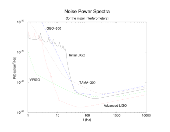
FIG. 7.: The predicetd noise power spectra for various interferometers. This Figure is adapted from [37]. $P(f)$ is what we called $S_{\cal N}$ and it is the quantity which should be compared with $S_{h}$. In this plot $f\equiv\nu$.

As we discussed in the previous Section, in order to have some hopes of detection we have to demand that the theoretical spectral density of the signal is larger than the spectral density of the noise. Let us then try to compare this value with the expected sensitivity of the interferometers possibly available in the near future. The power spectrum of our signal is too small to be seen by TAMA-300, GEO-600, and VIRGO. By correlating different detectors the sensitivity can increase also by a large factor [39, 40, 41]. However, the published results on the foreseen sensitivities at $\nu_{I}$ are far too large to be relevant for our background [26]. By comparing Fig. 6 with Fig. 7 we can argue that only the advanced LIGO detectors are closer to our predicted spectral density and that our signal in generally smaller than the advanced LIGO sensitivity. The two (identical) LIGO detectors are under construction in Handford (Washington) and in Livingston (Lousiana). After various years of operation the detectors will be continuously upgraded reaching, hopefully, the so-called advanced level of sensitivity.

Let us estimate the strength of our background for a frequency of the order of $0.1$ kHz –$1$ kHz. Let us assume that the energy density of the stochastic background is the maximal compatible with the nucleosynthesis indications. The graviton energy density (in critical units) at a frequency $\nu_{I}\sim 0.1$–$1$ kHz is then

$$\Omega_{{\rm GW}}(\nu_{I},\eta_{0})~{}h_{0}^{2}=2.29~{}10^{-15}~{}N_{s}^{-3/4}~{}\bigl{[}-19.7+0.25~{}\ln{N_{s}}\bigr{]}^{2},~{}~{}~{}~{}~{}\nu_{I}=0.1~{}{\rm kHz},$$ (5.1)

$$\Omega_{{\rm GW}}(\nu_{I},\eta_{0})~{}h_{0}^{2}=2.29~{}10^{-14}~{}N_{s}^{-3/4}~{}\bigl{[}-17.4+0.25~{}\ln{N_{s}}\bigr{]}^{2},~{}~{}~{}~{}\nu_{I}=1~{}{\rm kHz}.$$ (5.2)

Suppose then that we correlate the two LIGO detectors for a period $\tau=4$ months. Then, the signal to noise ratio (squared) can be expressed as [39, 40, 41]

$$\biggl{(}\frac{S}{N}\biggr{)}^{2}=\frac{9H_{0}^{4}}{50\pi^{4}}\tau\int_{0}^{\infty}d\nu\frac{\gamma^{2}(\nu)\Omega^{2}_{{\rm GW}}(\nu,\eta_{0})}{\nu^{6}S^{(1)}_{{\cal N}}(\nu)S^{(2)}_{{\cal N}}(\nu)}.$$ (5.3)

The function $\gamma(\nu)$ is called the overlap function. It takes into account the difference in location and orientation of the two detectors. It has been computed for the various pairs of LIGO-WA, LIGO-LA, VIRGO and GEO-600 detectors [41]. For detectors very close and parallel, $\gamma(\nu)=1$. Basically, $\gamma(\nu)$ cuts off the integrand of Eq. (5.3) at a frequency $2\pi\nu$ of the order of the inverse separation between the two detectors. For the two LIGO detectors, this cutoff is around 60 Hz. $S^{(1,2)}_{{\cal N}}$ are the noise spectral densities of the two LIGO detectors and since the two detectors are supposed to be identical we will have that $S^{(1)}_{{\cal N}}(\nu)=S^{(2)}_{{\cal N}}(\nu)$. In order to detect a stochastic background with $90\%$ confidence we have to demand $S/N\raise 1.72218pt\hbox{$>$}\kern-6.99997pt\lower 2.6694pt\hbox{$\sim$}1.65$. Now in order to estimate the signal to noise ratio we need to estimate numerically the integral appearing in Eq. (5.3). We know the theoretical spectrum since we just estimated it. The noise spectral densities of the LIGO detectors are not of public availability so that we cannot perform numerically this integral. In the case of a flat energy spectrum we have that the minimum $\Omega_{{\rm GW}}$ detectable in $\tau=4$ months is given, with $90~{}\%$ confidence, by $\Omega_{{\rm GW}}(\nu_{I},\eta_{0})=5\times 10^{-6}h^{-2}_{0}$ (for the initial LIGO detectors) and by $\Omega_{{\rm GW}}(\nu,\eta_{0})=5\times 10^{-11}h^{-2}_{0}$ (for the advanced LIGO detectors). For a correct comparison we should not confront Eqs. (5.1) and (5.2) with the sensitivities of the LIGO detectors to flat energy spectra but rather with the sensitivities obtained from Eq. (5.3) in the case of our specific energy spectrum reported in Eqs. (3.16).

Let us then compare, for illustration Eqs. (5.1) and (5.2) with the sensitivity to a flat energy spectrum even if this is not completely correct. The idea is to discuss, at fixed frequencies, the maximal signal provided by Eqs. (5.1)–(5.2) for different values of $R$.

FIG. 8.: With the two full thin lines we illustrate $\log{h^{2}_{0}\Omega_{{\rm GW}}(\nu_{I},\eta_{0})}$ as a function of $\log{N_{s}}$ for frequencies $\nu_{I}=0.1$ kHz according to Eqs. (5.1)–(5.2). The full thick lines represents the sensitivity of the LIGO detectors and of the advanced LIGO detectors to an energy density with flat frequency spectrum. From top to bottom the thick lines refer, respectively, to $h^{2}_{0}\Omega_{{\rm GW}}=5\times 10^{-6}$ and to $h^{2}_{0}\Omega_{{\rm GW}}=5\times 10^{-11}$. In order to be detected, the theoretical signal has to be above the thick line(s). We see that the region between the two thin lines does not overlap with the sensitivity of the upgraded LIGO detectors by, roughly, 1.5 orders of magnitude.

This comparison is illustrated in Fig. 8. For the allowed range of variation of $N_{s}$ our signal lies always below (of roughly $1.5$ orders of magnitude) the predicted sensitivity for the detection, by the advanced LIGO detectors, of an energy density with flat slope. The main uncertainty in this analysis is however the spectral behavior of the sensitivity for a spectrum which, unlike the one used for comparison, is not flat. It might be quite interesting to perform this calculation in order to see which is the precise sensitivity of the LIGO detectors to a spectral energy density as large as $10^{-12}$ and rising as $(\nu/\nu_{r})\ln{(\nu/\nu_{1})}$ in a frequency range $1$ Hz–$1$ kHz.

If we move from the kHz region to the GHz region the signal gets much larger than in the ordinary inflationary models. Moreover, the energy spectrum exhibits a quite broad peak whose typical amplitude can be as large as (but smaller then) $0.5\times~{}10^{-5}$. The spike (corresponding to the maximum of the peak) is located at a frequency of the order of $350~{}R^{-1/4}$ GHz.

On top of the interferometric detectors there are other types of detectors which are operating at the moment or might be operating in the future. The available upper limits on the strength of a stochastic background of relic gravitons come from the (cryogenic) resonant-mass detectors. In particular EXPLORER, while operating at CERN, provided an upper (direct) bound on the graviton energy density. The frequency $\nu_{B}$ relevant for this type of detectors is among $907$ and $923$Hz. By analyzing the 1991–1994 data of the EXPLORER antenna, the Rome group of G. Pizzella got a bound on the strength of the gravitons energy density of the order of $h_{0}^{2}\Omega_{{\rm GW}}\raise 1.72218pt\hbox{$<$}\kern-8.00003pt\lower 2.6694pt\hbox{$\sim$}300$. This bound, as it is, is not crucial since we know that the graviton energy density should be much lower, however we stress that this is direct bound from an operating device. Moreover, by correlating two bar detectors with the same features (like EXPLORER, NAUTILUS or AURIGA ) it is not excluded that a very interesting sensitivity of $h_{0}^{2}\Omega_{{\rm GW}}\sim 10^{-3}$ will be reached.

The particular spectral shape of the signal coming from quintessential inflation seems to point towards the use of electromagnetic detectors and, in particular of microwave cavities. A typical signature of the background we are discussing in the present paper is that the peak frequency (which almost saturates the nucleosynthesis bound) occurs for frequencies of the order of $\nu_{1}=3.58\times 10^{11}R^{-1/4}$ Hz. We can say that, very roughly, the size of the GW detectors is not only determined by construction requirement but also by the typical frequency range of the spectrum we ought to explore. In this sense the large separation between the two LIGO detectors is connected with the fact that the explored frequency range is of the order of $100$ Hz. Thus, if we deal with frequencies which are of the order of the GHz we can expect small detectors to be, theoretically, a viable option.

Microwave cavities can be used as GW detectors in the GHz frequency range [43, 45]. These detectors consist of an electromagnetic resonator, with two levels whose frequencies $\nu_{s}$ and $\nu_{a}$ are both much larger than the frequency $\nu_{{\rm GW}}$ of the gravitational wave to be detected. In the case of [43] the two levels are achieved by coupling two resonators one symmetric in the electric fields and the other antisymmetric. Indeed, in the case of cylindrical microwave cavities there are different normal oscillations of the electric fields. In [43] the relevant mode for the experimental apparatus is the ${\rm TE}_{011}$ according to the terminology usually employed in electrodynamics in order to identify normal modes of a cavity corresponding to different boundary conditions [44]. There were published results reporting the construction of such a detector [46]. In this case $\nu_{{\rm GW}}=10$ GHz and $\Delta\nu=\nu_{s}-\nu_{a}\sim 1$ MHz. In this experiment a sensitivity of fractional deformations $\delta x/x$ of the order of $10^{-17}$ was observed using an integration time $\Delta t\sim 10^{3}$ sec. The sensitivity to fractional deformations can be connected to the sensitivity for the observation of a monochromatic gravitational wave of frequency $\nu_{{\rm GW}}$. Following [46] we can learn that the sensitivity to fractional deformations is a function of $P_{a}$ and $P_{s}$ ( the powers stored in the symmetric and antisymmetric levels), $Q$ (the quality factor of the cavity [44] and which gives rate of dissipation of the power stored in the cavity). If we would assume, as in [46] $Q\sim 10^{9}$, $P_{a}\sim 10^{-21}$ Watt $P_{s}=2.4\times 10^{-2}$ Watt , we would get $\delta h\sim 10^{-17}$.

There, are at the moment, no operating prototypes of these detectors and so it is difficult to evaluate their sensitivity. The example we quoted [46] refers to 1978. We think that possible improvements in the $Q$ factors can be envisaged (we see quoted values of the order of $10^{12}$ which would definitely represent a step forward for the sensitivity). In spite of the fact that improvements can be foreseen we can notice immediately that, perhaps, to look in the highest possible frequency range of our model is not the best thing to do. In fact from Eq. (4.1) we can argue that in order to detect a signal of the order of $h^{2}_{0}\Omega_{{\rm GW}}\sim 10^{-6}$ at a frequency of $1$ GHz, we would need a sensitivity of the order of $\delta h\sim 10^{-30}$. Moreover as stressed in [47] the thermal noise should be properly taken into account in the analysis of the outcome of these microwave detectors. Indeed, as noticed from the very beginning [46], the thermal noise is one of the fundamental source of limitation of the sensitivity. An interesting strategy could be to decrease the operating frequency range of the device by going at frequencies of the order of $1$ MHz. Based on the considerations of [43] we can say that by taking high quality resonators the foreseen sensitivity can be as large as $h^{2}_{0}\Omega_{{\rm GW}}\sim 10^{-4}$. This sensitivity, though still above our signal, would be quite promising.

VI Graviton Spectra for quasi-de Sitter Phases

During an inflationary phase the evolution is not exactly of de Sitter type. We want to understand how the slope of the energy density of the relic graviton background will be modified by the slow-rolling corrections for frequencies accessible to the forthcoming interferometers. In general the deviations from a de Sitter stage can be induced either because of the specific inflationary model or because of the slow-rolling corrections whose strength can be described in terms of the so-called slow-rolling parameters

$$\alpha=-\frac{\dot{H}}{H^{2}}<~{}1,~{}~{}~{}\beta=\frac{\ddot{\phi}}{H\dot{\phi}}<~{}1,$$ (6.1)

where $H=(\ln{a})^{\cdot}$ is the Hubble parameter in cosmic time, $\phi$ is the inflaton and the dot denotes derivation with respect to cosmic time. In the slow rolling approximation the inflaton evolution is dominated by the scalar field potential according to the (approximate) equations

$$3H\dot{\phi}+\frac{\partial V}{\partial\phi}\simeq 0,~{}~{}~{}M_{P}^{2}H^{2}\simeq V.$$ (6.2)

In this approximation $H$ is not exactly constant but it slowly decreases leading to what we called quasi de Sitter phase. The evolution equation of the mode function can be written, by using the definition of $\alpha$ as

$$\psi^{\prime\prime}+\bigl{[}k^{2}-2~{}a^{2}~{}H^{2}\bigl{(}1-\frac{\alpha}{2}\bigr{)}\bigr{]}\psi=0.$$ (6.3)

As we can see, the time-dependent frequency appearing in the mode function contains two contribution: the first one ( i.e. $2a^{2}H^{2}=2/\eta^{2}$) is the term coming from a pure de Sitter phase, the second one, proportional to $\alpha$, is the correction.

In short the logic is the following. The quasi de Sitter phase modifies (through and $\alpha$-dependent correction) the index of the Hankel functions whose precise value ( equal to $1.5$ in the pure de Sitter phase) gets slightly smaller than $1.5$. From the sign of the correction appearing in Eq. (6.3) we can argue that the quasi de Sitter nature of the inflationary phase will lead to a decrease in the slope of the energy spectrum. The question is how much the slope of the hard branch will be affected, or, more precisely, how much smaller than one will it be the slope of the hard branch of the graviton energy density.

The answer to this question will of course depend upon the specific inflationary model since the size of the slow-rolling corrections can vary from one inflationary potential to the other. Notice that our concern is different from the one usually present [48, 49, 50, 51] in the context of ordinary inflationary models where the slow-rolling corrections are taken into account in the soft branch of the spectra (namely at sufficiently large scales). Indeed, for flat spectra the most significant bounds come from the infra-red, whereas, in our case the most significant bounds are in the ultraviolet and we have to understand how the scales which re-enter in the stiff phase are affected by the quasi-de Sitter nature of the inflationary phase. Of course, we could also discuss the slow-rolling coprrections to the soft branch of our spectrum, but, they are, comparatively, less relevant (for the structure of the spike) than the correction to the hard branch.

As usual, the slow-rolling corrections not only affect the mode function evolution but also the definition of conformal time itself, namely we will have

$$\eta=\int\frac{dt}{a}=\int\frac{da}{a^{2}H}=-\frac{1}{aH}+\int\alpha\frac{da}{a^{2}H}.$$ (6.4)

By using the fact that $M_{P}^{2}\dot{H}=-(3/2)\dot{\phi}^{2}$ and the fact that $\beta<1$ we can connect directly $\alpha$ to the slope of the potential

$$\alpha=-\frac{\dot{H}}{H}=\frac{M_{P}^{2}}{6}\biggl{(}\frac{\partial\ln{V}}{\partial\phi}\biggr{)}^{2}.$$ (6.5)

Since we are interested in the lowest order slow-rolling correction we will assume that $\alpha$ and $\beta$ are constants. This is a simplification which will not affect (numerically ) the slope of the spectrum. In the case of inflationary models with chaotic and exponential potential it can be shown that the “running” of $\alpha$ with $\phi$ (and, therefore, with the wavenumber $k$) will affect the spectral slopes with a term which is of the order of $1/N^{2}$ where $N$ is the number of inflationary e-folds [51, 52, 53]. If $\alpha$ is constant then we have that $\eta^{-1}=-(aH)/(1+\alpha)$ which leads, once inserted in Eq. (6.3)

$$\psi^{\prime\prime}+\bigl{[}k^{2}-\frac{\nu^{2}-\frac{1}{4}}{\eta^{2}}\bigr{]}=0,~{}~{}~{}{\rm with}~{}~{}~{}\nu=\frac{3}{2}+\alpha,$$ (6.6)

where the expression of $\nu$ holds for $\alpha<1$.

Let us examine now the quasi-de Sitter nature of different inflationary scenarios. An inflationary potential of chaotic form

$$V(\phi)=\frac{\phi^{n}}{n!},$$ (6.7)

will lead to $\alpha=(M_{P}^{2}/6)(n^{2}/\phi^{2})$. Let us take the value of $\alpha$ the one corresponding to modes crossing the horizon around $20$–$25$ e-folds before the end of inflation. The reason for this choice is very simple. We want to understand how is modified the slope of the energy spectrum for scales larger than (and of the order of) the ones probed by the interferometers. A simple calculation shows that, for instance, the LIGO/VIRGO scale crosses the horizon roughly $21$ e-folds before the end of inflation. The end of inflation occurs when $\alpha(\phi_{\rm end})=1$. Thus, at the end of inflation $\phi^{2}_{{\rm end}}=(M_{P}^{2}/6)n^{2}$. By solving consistently Eqs. (6.2) with the potential (6.7) we get easily that the number of inflationary e-folds at a given value of $\phi$ is given by

$$N(\phi)=\int_{\phi}^{\phi_{{\rm end}}}\frac{da}{a}=\frac{3}{2M_{P}^{2}n}(\phi^{2}-\phi^{2}_{{\rm end}}).$$ (6.8)

From this last equation we can determine easily $\phi_{21}$ and then, by inserting $\phi^{2}_{{\rm end}}$, $\alpha$ turns out to be

$$\alpha=\frac{n}{n+84},$$ (6.9)

which is of the order of $0.02$ for $n=2$ , of the order of $0.04$ for $n=4$ and so on. Another example could be the one of an exponential potential. Using the definition of $\alpha$ from Eq. (6.5) we have that for an exponential potential of the form

$$V(\phi)=\exp{\bigl{[}\frac{1}{q}\frac{\phi}{M_{P}}\bigr{]}},$$ (6.10)

will lead to $\alpha=1/q^{2}$.

With these results we can easily compute the corrections to the hard branch of the spectrum. The spectral energy density will be

$$\Omega_{{\rm GW}}(\omega,\eta_{0})=\Omega_{\gamma}(\eta_{0})f(\alpha,\lambda,R)\bigl{(}\frac{\omega}{\omega_{r}}\bigr{)}^{1-2\alpha}\ln^{2}{\bigl{(}\frac{\omega}{\omega_{1}}\bigr{)}},~{}~{}~{}{\rm with}$$ (6.11)

$$f(\alpha,\lambda,R)=\frac{9}{\pi^{4}}~{}\bigl{(}\alpha+\frac{3}{2}\bigr{)}^{2}~{}2^{2\alpha}~{}|\Gamma(\frac{3}{2}+\alpha)|^{2}\lambda^{1-2\alpha}R^{-2\alpha}\bigl{(}\frac{g_{{\rm dec}}}{g_{r}}\bigr{)}^{1/3}.$$ (6.12)

The power spectrum and the associated spectral density can be computed from using the techniques already discussed in the previous Sections. Some authors call $-2\alpha$ the corrections to the spectral index. Eq. (6.12) tells us that the corrections arising during a quasi-de Sitter phase always go in the direction of making the maximal slope of the hard branch slightly smaller than one by a factor $0.08$ (for instance in the case the case of $\phi^{4}$ potential). In the case of exponential potential the magnitude of the correction to the slope is controlled by $q^{2}$. Again we see that for reasonable values of $q^{2}$ like $q^{2}=5,~{}10,...$ [5] the correction are again small and, at most, of the order of few percents.

VII Concluding Remarks

In this paper we computed the relic graviton spectra in quintessential inflationary models. We showed that the energy spectra possess a hard branch which increases in frequency. Large energy densities in relic gravitons can be expected in this class of models. The spike of the energy spectrum can be as large as $h_{0}^{2}\Omega_{{\rm GW}}\simeq 10^{-6}$ at a typical (present) frequency $\nu_{1}=358\times R^{-1/4}$ GHz. The spectral amplitude at the interferometers frequencies is just below the value visible by the upgraded LIGO detectors. Since a large amount of energy density can be stored around the GHz the use of small electromagnetic detectors for the detection of such a background seems more plausible. In particular microwave cavities should be considered as a possible candidate. Our investigation also hints that the sensitivities of the advanced LIGO detectors to energy spectra increasing, in frequency, as $\nu\ln\nu$ should be precisely computed by convolving our spectra with the noise power spectra of the detectors.

A Relic Gravitons Correlation Functions

In this Appendix we concentrate some of the more technical derivations concerning the spectral properties of the relic gravitons which can be characterized through their energy density in critical units or through the two point correlation function of the amplified tensor fluctuations of the metric. We want to give explicit derivations of these quantities and of their relations.

Let us start from the canonical action describing relic gravitons in a curved metric of Friedmann-Robertson-Walker type. GW, being pure tensor modes of the geometry, only couple to the curvature but not to the matter sources. Their effective action can be obtained by perturbing the Einstein-Hilbert action

$$S=-\frac{1}{6l_{P}^{2}}\int\sqrt{-g}Rd^{4}x,$$ (A.1)

to second order in the amplitude of the tensor fluctuations of the metric

$$g_{\mu\nu}(\vec{x},\eta)\rightarrow\overline{g}_{\mu\nu}(\eta)+\delta g^{(T)}_{\mu\nu}(\vec{x},\eta),~{}~{}~{}\delta g_{\mu\nu}=h_{\mu\nu},~{}~{}~{}h_{\mu 0}=0.$$ (A.2)

Pure tensor fluctuations of the metric (with two physical polarizations) can be constructed by using a symmetric three-tensor $h_{ij}$ satisfying the constraints $h_{i}^{i}=0$, $\nabla_{i}h_{j}^{i}=0$ (where $\nabla_{i}$ is the covariant derivative with respect to the three-dimensional background metric). The action perturbed to second order in the amplitude of the tensor fluctuations becomes

$$\delta^{(2)}S^{(T)}=\frac{1}{24l_{P}^{2}}\int d^{4}x\sqrt{-\overline{g}}\partial_{\alpha}h_{ij}\partial_{\beta}h^{ij}\overline{g}^{\alpha\beta}.$$ (A.3)

We can construct two independent scalars corresponding to the two polarization states of the gravitational waves:

$$h_{ij}(\vec{x},\eta)=h_{\oplus}(\vec{x},\eta)q_{ij}^{(1)}(\vec{x})+h_{\otimes}(\vec{x},\eta)q_{ij}^{(2)}(\vec{x}),$$ (A.4)

where

$$q_{(1)}^{ij}(\vec{x})=-[e_{1}^{i}(\vec{x})e^{j}_{1}(\vec{x})-e_{2}^{j}(\vec{x})e^{i}_{2}(\vec{x})],~{}~{}~{}q_{(2)}^{ij}(\vec{x})=-[e_{1}^{i}(\vec{x})e^{j}_{1}(\vec{x})+e_{2}^{j}(\vec{x})e^{i}_{2}(\vec{x})].$$ (A.5)

In these coordinates $\vec{e}_{1}$, $\vec{e}_{2}$ and $\vec{e}_{3}$ form an orthonormal set of vectors. In the previous decomposition we assumed the wave to propagate along $\vec{e}_{3}$. So the perturbed action can also be written, in units of $6l_{P}^{2}=1$, as

$$\delta^{(2)}S^{(T)}=\frac{1}{2}\int d^{4}x\sqrt{-\overline{g}}[\partial_{\alpha}h_{\oplus}\partial_{\beta}h_{\oplus}\overline{g}^{\alpha\beta}+\partial_{\alpha}h_{\otimes}\partial_{\beta}h_{\otimes}\overline{g}^{\alpha\beta}].$$ (A.6)

The associated energy-momentum tensor can be written as [55, 56]

$$T_{\mu\nu}=\frac{1}{2}\biggl{[}\partial_{\mu}h_{\oplus}\partial_{\nu}h_{\oplus}+\partial_{\mu}h_{\otimes}\partial_{\nu}h_{\otimes}-\overline{g}_{\mu\nu}\biggl{(}\overline{g}^{\alpha\beta}\partial_{\alpha}h_{\oplus}\partial_{\beta}h_{\oplus}+\overline{g}^{\alpha\beta}\partial_{\alpha}h_{\otimes}\partial_{\beta}h_{\otimes}\biggr{)}\biggr{]}.$$ (A.7)

The canonically normalized graviton field can be written as $\mu_{ij}=ah_{ij}$ and its corresponding action reads

$$\delta^{(2)}S^{(T)}=\frac{1}{2}\int d^{3}xd\eta\biggl{[}\eta^{\alpha\beta}\partial_{\alpha}\mu_{\oplus}\partial_{\beta}\mu_{\oplus}+\eta^{\alpha\beta}\partial_{\alpha}\mu_{\otimes}\partial_{\beta}\mu_{\otimes}+\frac{a^{\prime\prime}}{a}(\mu_{\oplus}^{2}+\mu_{\otimes}^{2})\biggr{]}.$$ (A.8)

With this form of the action we can promote the classical canonical normal modes to field operators obeying the standard (equal time) commutation relations. The Fourier expansion of the field operators will then look

$$\hat{\mu}_{\oplus}(\vec{x},\eta)=\frac{1}{(2\pi)^{3/2}}\int d^{3}k\biggl{[}\hat{\mu}_{\oplus}(k,\eta)e^{i\vec{k}\cdot\vec{x}}+\hat{\mu}_{\oplus}^{\dagger}(k,\eta)e^{-i\vec{k}\cdot\vec{x}}\biggr{]},$$ (A.9)

$$\hat{\mu}_{\otimes}(\vec{x},\eta)=\frac{1}{(2\pi)^{3/2}}\int d^{3}k\biggl{[}\hat{\mu}_{\otimes}(k,\eta)e^{i\vec{k}\cdot\vec{x}}+\hat{\mu}_{\otimes}^{\dagger}(k,\eta)e^{-i\vec{k}\cdot\vec{x}}\biggr{]},$$ (A.10)

where $\hat{\mu}_{\oplus}(k,\eta)=\psi_{\oplus}(k,\eta)\hat{a}_{\oplus}(\vec{k})$ and $\hat{\mu}_{\otimes}(k,\eta)=\psi_{\otimes}(k,\eta)\hat{a}_{\otimes}(\vec{k})$. The creation and annihilation operators follow the usual commutation relations namely

$$[\hat{a}_{\lambda}(\vec{k}),\hat{a}_{\sigma}^{\dagger}(\vec{p})]=\delta_{\lambda\sigma}\delta^{(3)}(\vec{k}-\vec{p}).$$ (A.11)

From the Heisenberg equations of motion for the field operators follow the evolution equations for the Fourier amplitudes

$$\psi^{\prime\prime}+[k^{2}-\frac{a^{\prime\prime}}{a}]\psi=0,$$ (A.12)

for each of the two physical polarizations. In most of the cosmological applications we will be dealing with $|a^{\prime\prime}/a|$ has a bell-like shape going to zero , for large conformal times, as $\eta^{-2}$. Eq. (A.12) can be be solved in two significant limits. The first one is for $k^{2}\ll|a^{\prime\prime}/a|$ corresponding to wavelength which are outside of the horizon (under the bell)

$$\psi(k,\eta)=A(k)a(\eta)+B(k)a(\eta)\int^{\eta}\frac{d\eta^{\prime}}{a^{2}},$$ (A.13)

where $A(k)$ and $B(k)$ are integration constants. For large momenta (i.e. $k^{2}\gg|a^{\prime\prime}/a|$) the general solution of Eq. (A.12) is

$$\psi(k,\eta)=\frac{1}{\sqrt{2k}}\bigl{[}\beta_{+}(k)e^{-ik\eta}+\beta_{-}(k)e^{ik\eta}\bigr{]},$$ (A.14)

where $\beta_{-}(k)$ and $\beta_{+}(k)$ are complex numbers and where the quantum mechanical normalization $1/\sqrt{2k}$ has been chosen. Therefore, if we start at $\eta\rightarrow-\infty$ with a positive frequency mode the evolution for $k^{2}\ll|a^{\prime\prime}/a|$ will mix the the positive frequency with the negative one and eventually we will end up, for $\eta\rightarrow+\infty$ with a superposition of positive and negative frequencies according to Eq. (A.14)

The two point correlation function of the graviton field operators can then be computed in Fourier space

$$\langle 0|\hat{\mu}_{\lambda}(\vec{k},\eta)\hat{\mu}_{\sigma}^{\dagger}(\vec{p},\eta)|0\rangle=|\psi_{\lambda}(k,\eta)|^{2}\delta_{\lambda\sigma}\delta^{(3)}(\vec{k}-\vec{p}).$$ (A.15)

Field modes with different wave-numbers are then statistically independent as a consequence of the graviton emission from the vacuum. Some authors refer to Eq. (A.15) as to the stochasticity condition which express the main statistical property of the graviton background. Within our quantum mechanical formalism we can also compute the two-point correlation function between field operators, namely

$$\xi(r)=\langle 0|\hat{\mu}_{ij}(\vec{x})\hat{\mu}^{ij}(\vec{x}+\vec{r})|0\rangle=\frac{1}{\pi^{2}}\int\frac{dk}{k}\frac{\sin{kr}}{kr}|\delta_{h}(k,\eta)|^{2},$$ (A.16)

where

$$|\delta_{\psi}(k,\eta)|^{2}=k^{3}(|\psi_{\oplus}(k,\eta)|^{2}+|\psi_{\otimes}(k,\eta)|^{2}),$$ (A.17)

is the power spectrum of the relic gravitons background summed over the physical polarizations.

Sometimes, to facilitate the transition to the quantities often used by the experimentalists, it is convenient to denote the gravitational wave amplitude, for each polarization, with

$$h(\vec{x},\eta)=\frac{1}{(2\pi)^{3/2}}\int d^{3}k~{}h(k,\eta)~{}e^{i\vec{k}\cdot\vec{x}},$$ (A.18)

where the reality condition implies $h^{\ast}(\vec{k})=h(-\vec{k})$. The statistical independence of waves with different wave vectors implies, in this formalism, that

$$\langle h_{\lambda}(\vec{k},\eta)h^{\ast}_{\sigma}(\vec{p},\eta)\rangle=|h_{\lambda}(k,\eta)|^{2}\delta_{\lambda\sigma}\delta^{(3)}(\vec{k}-\vec{p}),~{}~{}~{}h_{\lambda}(k,\eta)=\frac{\psi_{\lambda}(k,\eta)}{a}.$$ (A.19)

Eq. (A.19) can be viewed as the classical limit of Eq. (A.15) where the quantum mechanical expectation values are replaced by ensemble averages. Notice that this concept can be made quite rigorous by taking the average of the graviton field over the coherent state basis. This procedure would be analogous to what is normally done in quantum optics in the context of the optical equivalence theorem [54].

The energy density (and pressure) of the relic graviton background can be easily obtained by taking the average of the energy momentum tensor. The energy density is

$$\rho_{GW}(\eta)=\langle 0|T_{00}|0\rangle,$$ (A.20)

which can also be written as

$$\rho_{GW}(\eta)=\langle 0_{\otimes}0_{\oplus}|\tau_{oo}|0_{\oplus}0_{\otimes}\rangle=$$ (A.21)

$$\frac{1}{16\pi^{3}~{}a^{2}}\int d^{3}k\Biggl{[}|h^{\prime}_{\oplus}(k,\eta)|^{2}+|h^{\prime}_{\otimes}(k,\eta)|^{2}+k^{2}\biggl{(}|h_{\oplus}(k,\eta)|^{2}+|h_{\otimes}(k,\eta)|^{2}\biggr{)}\Biggr{]}.$$ (A.22)

If we insert the asymptotic expression of the mode function of each polarization for large (positive) conformal times we get, from Eq. (A.22),

$$\rho_{GW}(\eta)=\int\frac{d\omega}{\omega}\omega^{4}\frac{|\beta_{-}(\omega)|^{2}}{\pi^{2}},~{}~{}~{}\omega=k/a,$$ (A.23)

from which we can define the logarithmic energy spectrum as

$$\frac{d\rho_{GW}(\omega,\eta)}{d\ln\omega}=\frac{\omega^{4}}{\pi^{2}}|\beta_{-}(\omega)|^{2},$$ (A.24)

(where we used the fact that $|\beta_{+}(\omega)|^{2}-|\beta_{-}(\omega)|^{2}=1$) By taking into account that the energy density of $\overline{n}(\omega)$ gravitons in the proper momentum interval $d\omega$ is given by

$$d\rho_{GW}=2\omega\overline{n}(\omega)\frac{d^{3}\omega}{(2\pi)^{3}},$$ (A.25)

$|\beta_{-}(k)|^{2}$ can be interpreted as the mean number of produced gravitons in a given frequency interval.

In order to compute the relation between $\Omega_{GW}(\omega,\eta)$ and $\delta_{h}(\omega,\eta)=\delta_{\psi}(\omega,\eta)/a(\eta)$ we can use Eq. (A.18). The energy density in gravity waves is given by

$$\rho_{GW}(\eta)=\frac{M_{P}^{2}}{6a^{2}}\langle{h^{\prime}}^{2}_{\otimes}+{h^{\prime}}^{2}_{\oplus}\rangle,$$ (A.26)

where the brackets indicate now ensemble average of the Fourier amplitudes. Using now Eq. (A.18) together with the stochasticity condition we obtain (after having divided by the critical energy density)

$$\Omega_{GW}(\omega,\eta_{0})=\frac{1}{6\pi^{2}}\bigl{(}\frac{\omega}{H_{0}}\bigr{)}^{2}|\delta_{h}(\omega,\eta_{0})|^{2}.~{}~{}~{}$$ (A.27)

where the $\eta_{0}$ is the present conformal time which appears since we want to refer everything to the present value of the Hubble constant. In comparing the signal coming from a particular model with the experimental sensitivities it turns out to be widely used the spectral density $S_{h}(\nu,\eta_{0})$. In order to define it let us assume that each polarization of the gravity wave amplitude can be written as

$$h(\nu)=\int dt~{}h(t)~{}e^{-2i\pi\nu t},$$ (A.28)

where $t$ is the cosmic time variable. Then the spectral amplitude can be defined as

$$\langle h(\nu)h^{\ast}(\nu^{\prime})\rangle=\frac{1}{2}\delta(\nu-\nu^{\prime})S_{h}(\nu).$$ (A.29)

By inserting this expression into Eq. (A.26) and by using the definition (A.29) we obtain

$$\Omega_{GW}(\nu,\eta_{0})=\frac{4\pi^{2}}{3H_{0}^{2}}\nu^{3}S_{h}(\nu,\eta_{0}).$$ (A.30)

This last equation implies that

$$S_{h}(\nu,\eta_{0})=8\times 10^{-37}\Omega_{GW}(\nu,\eta_{0})h_{0}^{2}\frac{{\rm Hz}^{2}}{\nu^{3}}$$ (A.31)

from which is clear that $S_{h}$ is measured in seconds.

B Relic Gravitons Spectra in the Ordinary Inflationary Case

Consider the model of an Universe evolving from a de Sitter stage of expansion to a matter-dominated phase passing through a radiation dominated phase. By requiring the continuity of the scale factors and of their first derivatives at the transition points we have that $a(\eta)$, in the three different temporal regions, can be represented as

$$a_{i}(\eta)=\biggl{[}-\frac{\eta_{1}}{\eta}\biggr{]},~{}~{}~{}{\rm for}~{}~{}~{}~{}~{}~{}~{}~{}~{}~{}~{}~{}~{}~{}~{}\eta<-\eta_{1}$$ (B.1)

$$a_{r}(\eta)=\frac{\eta+2\eta_{1}}{\eta_{1}},~{}~{}~{}{\rm for}~{}~{}~{}~{}~{}-\eta_{1}<~{}\eta~{}<\eta_{2}$$ (B.2)

$$a_{m}(\eta)=\frac{(\eta+\eta_{2}+4\eta_{1})^{2}}{4\eta_{1}(\eta_{2}+2\eta_{1})},~{}~{}~{}{\rm for}~{}~{}~{}~{}~{}~{}~{}~{}\eta>\eta_{2}$$ (B.3)

where $-\eta_{1}$ and $\eta_{2}$ mark, respectively, the onset of the radiation-dominated phase and the decoupling time.

In order to compute the graviton spectra in this model we have to estimate the amplification of the graviton mode function induced by the background evolution reported in Eq. (B.3). The solution of Eq. (A.12) in the three temporal regions is given by

$$\psi_{i}(x)=\frac{p}{\sqrt{2k}}\sqrt{x}H_{\nu}^{(2)}(x),$$ (B.4)

$$\psi_{r}(y)\frac{1}{\sqrt{2k}}[B_{+}e^{-iy}+B_{-}e^{iy}],$$ (B.5)

$$\psi_{m}(z)\frac{1}{\sqrt{2k}}\sqrt{z}[q^{\ast}c_{+}H_{\mu}^{(2)}(z)+qc_{-}H_{\mu}^{(1)}(z)],$$ (B.6)

where

$$x=k\eta,~{}~{}~{}y=k(\eta+2\eta_{1}),~{}~{}~{}z=k(\eta+\eta_{2}+4\eta_{1}).$$ (B.7)

and $H^{(1,2)}_{\nu,\mu}$ are the Hankel functions [57, 58] of first and second kind. In the case of the background given by Eq. (B.3) the Bessel indeces $\nu$ and $\mu$ are both equal to $3/2$ but we like to keep them general in light of the applications reported in the present paper.

Notice that in Eq. (B.6) we included

$$p=\sqrt{\frac{\pi}{2}}e^{-i\frac{\pi}{4}(1+2\nu)},~{}~{}~{}q=\sqrt{\frac{\pi}{2}}e^{i\frac{\pi}{4}(1+2\mu)},$$ (B.8)

ensuring that the large time limit of the mode function is the one dictated by quantum mechanics (i.e. $e^{i\pm k\eta}/\sqrt{2k}$) without any extra phase or extra (constant) coefficient.

The constants appearing in Eq. (B.6) are fixed by the quantum mechanical normalization imposed during the de Sitter phase, and then, in order to compute the amplification we have to match the various expressions of the mode functions (and of their first derivatives) in $\eta=-\eta_{1}$ and in $\eta=\eta_{2}$. By doing this we get the expression of the amplification coefficients. By firstly looking at modes which went outside of the horizon during the de Sitter phase and re-entered during the radiation dominated phase (i.e. modes $2\pi/\eta_{1}<k<2\pi/\eta_{2}$) we have that $B_{\pm}$ are given by

$$B_{\mp}=\frac{e^{\mp ix_{1}}}{2}p~{}\bigl{\{}H^{(2)}_{\nu}(-x_{1})\bigl{[}\sqrt{-x_{1}}\mp\frac{i}{\sqrt{-x_{1}}}\bigl{(}\nu+\frac{1}{2}\bigr{)}\bigr{]}\pm i\sqrt{-x_{1}}H^{(2)}_{\nu+1}(-x_{1})\bigl{\}}$$ (B.9)

We are interested in the $B_{-}$ which measures the amount of mixing between positive and negative frequency modes and whose square modulus can be interpreted as the mean number of produced gravitons. Moreover, we want to evaluate $B_{-}$ in the small argument limit (i.e. $x_{1}\ll 1$) which is the one physically relevant. The result is

$$B_{-}(k)=\frac{2^{\nu-1}}{\sqrt{2\pi}}\Gamma(\nu)\biggl{(}\frac{1}{2}-\nu\biggr{)}e^{-i\frac{\pi}{4}(1+2\nu)}|k\eta_{1}|^{-\frac{1}{2}-\nu},$$ (B.10)

where $\Gamma(\nu)$ is the Euler Gamma function. In the case of a pure de Sitter background we get, indeed,

$$B_{-}(k)=-\frac{e^{-i\pi}}{2}|k\eta_{1}|^{-2}.$$ (B.11)

In order to compute the spectrum of the relic gravitons crossing the horizon during the matter dominated epoch we have to consider a further transition by matching $\psi_{r}(y)$ and $\psi_{m}(z)$ (and their first derivatives) in $\eta=\eta_{2}$. The result is that

$$c_{-}=-\frac{i}{2}(B_{+}-B_{-})\sqrt{z_{2}}H^{(2)}_{\mu}(z_{2})q,$$ (B.12)

where we reported only the dominant part in the $x_{1}\ll 1$ and $z_{2}\ll 1$ limit. By performing the limit explicitly we get

$$|c_{-}(k)|=\frac{\Gamma(\mu)~{}\Gamma(\nu)}{2\pi^{2}}2^{\mu+\nu}\bigl{(}\frac{1}{2}-\nu\bigr{)}|q||p||k\eta_{1}|^{-\nu-\frac{1}{2}}~{}|k\eta_{2}|^{-\mu+\frac{1}{2}}.$$ (B.13)

In the case of the model of Eq. (B.3) we have that the energy density of the created gravitons in critical units at the present observation time

$$\Omega(\nu,\eta_{0})=\frac{1}{\rho_{c}}\frac{d\rho_{GW}}{d\ln\nu},$$ (B.14)

can be computed by inserting into Eq. (A.24) the expressions of the mixing coefficients of Eqs. (B.10)–(B.12), with the result that

$$\Omega_{GW}(\nu,\eta_{0})\simeq\Omega_{\gamma}(\eta_{0})\biggl{(}\frac{H_{1}}{M_{P}}\biggr{)}^{2},~{}~{}~{}~{}~{}~{}~{}~{}~{}~{}~{}\nu_{{\rm dec}}<\nu<\nu_{1}$$ (B.15)

$$\Omega_{GW}(\nu,\eta_{0})\simeq\Omega_{\gamma}(\eta_{0})\biggl{(}\frac{H_{1}}{M_{P}}\biggr{)}^{2}\biggl{(}\frac{\nu_{{\rm dec}}}{\nu}\biggr{)}^{2},~{}~{}~{}\nu_{0}<\nu<\nu_{{\rm dec}}$$ (B.16)

This spectrum is reported in Fig. 1. The soft branch and the hard branch defined in the Introduction do correspond, respectively, to the two frequency ranges $\nu_{0}<\nu<\nu_{{\rm dec}}$ and $\nu_{{\rm dec}}<\nu<\nu_{1}$.

C Transition from Inflation to Stiff Phase: Accurate Mixing Coefficients

In order to determine the six matching coefficients appearing in Eq. (3.10) we have to match the mode function $\psi$ and its first derivative in $\eta=-\eta_{1}$, $\eta=\eta_{r}$ and $\eta=\eta_{{\rm dec}}$. The results of this calculation are reported in the present section. Consider first the amplification leading to the hard branch of the spectrum. The mixing coefficients are given by

$$A_{-}(k)=-\frac{\pi}{4\sqrt{2}}e^{-\frac{i}{2}\pi(\nu+1)}\bigl{\{}H_{0}^{(2)}\bigl{(}\frac{x_{1}}{2}\bigr{)}\bigl{[}x_{1}H^{(2)}_{\nu+1}(-x_{1})-\nu H^{(2)}_{\nu}(-x_{1})\bigr{]}-x_{1}H^{(2)}_{1}\bigl{(}\frac{x_{1}}{2}\bigr{)}H^{(2)}_{\nu}(-x_{1})\bigr{\}}.$$ (C.1)

$$A_{+}(k)=\frac{\pi}{4\sqrt{2}}e^{-\frac{i}{2}\pi\nu}\bigl{\{}H^{(1)}_{0}\bigl{(}\frac{x_{1}}{2}\bigr{)}\bigl{[}x_{1}H^{(2)}_{\nu+1}(-x_{1})-\nu H^{(2)}_{\nu}(-x_{1})\bigr{]}-x_{1}H^{(1)}_{1}\bigl{(}\frac{x_{1}}{2}\bigr{)}H^{(2)}_{\nu}(-x_{1})\bigr{\}}.$$ (C.2)

The small argument limit of $A_{-}$ (directly relevant for the estimate of the graviton spectrum in the hard branch) can be easily obtained and it turns out to be

$$A_{-}(k)\sim\frac{3\nu}{\pi}2^{\nu-\frac{3}{2}}e^{-\frac{i}{2}\pi(2\nu+1)}\Gamma(\nu)x_{1}^{-\nu}\ln{x_{1}}.$$ (C.3)

In order to derive the previous and the following expressions it is useful to bear in mind that the Wronskian of the Hankel functions is given by

$${\cal W}\bigl{[}H^{(1)}_{\alpha}(r),H^{(2)}_{\alpha}(r)\bigr{]}=H^{(1)}_{\alpha+1}(r)H^{(2)}_{\alpha}(r)-H^{(1)}_{\alpha}(r)H^{(2)}_{\alpha+1}(r)=-\frac{4i}{\pi r},$$ (C.4)

for a generic argument $r$ and for a generic Bessel index $\alpha$. In this calculation it is also useful to recall that the small argument limit of the Hankel functions is

$$H^{(1,2)}_{\alpha}(r)\sim\biggl{(}\frac{r}{2}\biggr{)}^{\alpha}\frac{1}{\Gamma(\alpha+1)}\mp\frac{i}{\pi}\Gamma(\alpha)\biggl{(}\frac{r}{2}\biggr{)}^{-\alpha},$$ (C.5)

where the minus (plus) refers to the Hankel function of first (second) kind. Notice that this formula is only valid for $\alpha\neq 0$. In this last case we have indeed that

$$H^{(1,2)}_{0}(r)\sim 1\mp\frac{2}{\pi}\ln{r}.$$ (C.6)

Let us now consider the following transition namely the one leading to the semi-hard branch of the spectrum. The exact expression of the mixing coefficients is, in this case,

$$B_{\pm}(k)=\frac{e^{\pm iy_{r}}}{2}\bigl{\{}\sqrt{y_{r}}\bigl{[}s^{\ast}A_{+}(k)H^{(2)}_{0}(y_{r})+sA_{-}(k)H_{0}^{(1)}(y_{r})\bigr{]}\pm i\bigl{[}s^{\ast}A_{+}(k)\bigl{(}\frac{1}{2\sqrt{y_{r}}}H^{(2)}_{0}(y_{r})-\sqrt{y_{r}}H^{(2)}_{1}(y_{r})\bigr{)}$$ (C.7)

$$+sA_{-}(k)\bigl{(}\frac{1}{2\sqrt{y_{r}}}H^{(1)}_{0}(y_{r})-\sqrt{y_{r}}H^{(1)}_{1}(y_{r})\bigr{)}\bigr{]}\bigr{\}}.$$ (C.8)

The small argument limit of $B_{-}$ leads to

$$B_{-}(k)=-e^{-i\pi\nu+i\frac{\pi}{4}}~{}\frac{3\nu}{2\sqrt{2\pi}}2^{\nu-\frac{3}{2}}\Gamma(\nu)~{}|k\eta_{r}|^{-\frac{1}{2}}~{}|k\eta_{1}|^{-\nu}\ln{\bigl{[}\frac{\eta_{1}}{\eta_{r}}\bigr{]}},$$ (C.9)

which becomes, in the case $\nu=\frac{3}{2}$,

$$B_{-}(k)=\frac{9}{8\sqrt{2}}~{}|k\eta_{r}|^{-\frac{1}{2}}~{}|k\eta_{1}|^{-\frac{3}{2}}\ln{\bigl{[}\frac{\eta_{1}}{\eta_{r}}\bigr{]}}.$$ (C.10)

Finally, let us compute the amplification coefficients in the case of the soft branch of the spectrum. In this case we have that the mixing coefficients are

$$c_{-}(k)=\frac{i}{2}\bigl{\{}\bigl{(}B_{+}(k)e^{-iy_{{\rm dec}}}+B_{-}(k)e^{iy_{{\rm dec}}}\bigr{)}\bigl{[}\bigl{(}\mu+\frac{1}{2}\bigr{)}\frac{q^{\ast}}{\sqrt{z_{{\rm dec}}}}H^{(2)}_{\mu}(z_{{\rm dec}})$$ (C.11)

$$-\sqrt{z_{{\rm dec}}}q^{\ast}H^{(2)}_{\mu+1}(z_{{\rm dec}})\bigr{]}+i\bigl{(}B_{+}(k)e^{-iy_{{\rm dec}}}-B_{-}(k)e^{iy_{{\rm dec}}}\bigr{)}\sqrt{z_{{\rm dec}}}q^{\ast}H^{(2)}_{\mu}(z_{{\rm dec}})\bigr{\}}.$$ (C.12)

$$c_{-}(k)=-\frac{i}{2}\bigl{\{}\bigl{(}B_{+}e^{-iy_{{\rm dec}}}+B_{-}(k)e^{iy_{{\rm dec}}}\bigr{)}\bigl{[}\bigl{(}\mu+\frac{1}{2}\bigr{)}\frac{q}{\sqrt{z_{{\rm dec}}}}H^{(1)}_{\mu}(z_{{\rm dec}})$$ (C.13)

$$-\sqrt{z_{{\rm dec}}}qH^{(1)}_{\mu+1}(z_{{\rm dec}})\bigr{]}+i\bigl{(}B_{+}(k)e^{-iy_{{\rm dec}}}-B_{-}e^{iy_{{\rm dec}}}\bigr{)}\sqrt{z_{{\rm dec}}}qH^{(1)}_{\mu}(z_{{\rm dec}})\bigr{\}}.$$ (C.14)

In the small argument limit we have

$$c_{-}(k)=-\frac{3\nu}{4\pi}2^{\mu+\nu-\frac{3}{2}}e^{-i\pi(\nu+2\mu)}\Gamma(\mu)\Gamma(\nu)|k\eta_{r}|^{-\frac{1}{2}}|k\eta_{1}|^{-\nu}|k\eta_{{\rm dec}}|^{-\mu+\frac{1}{2}}\ln{\bigl{[}\frac{\eta_{1}}{\eta_{r}}\bigr{]}},$$ (C.15)

which becomes, in the case $\mu=3/2$,

$$c_{-}(k)=-\frac{9~{}\pi}{16\sqrt{2}}e^{-i\frac{9}{2}\pi}|k\eta_{1}|^{-\frac{3}{2}}|k\eta_{{\rm dec}}|^{-1}|k\eta_{r}|^{-\frac{1}{2}}\ln{\bigl{[}\frac{\eta_{1}}{\eta_{r}}\bigr{]}}.$$ (C.16)

The derivations we just reported are the basis for the results presented in Section III.

REFERENCES

- [1] A. Abramovici et al. , Science, 256, 325 (1992).
- [2] C. Bradaschia et al. , Nucl. Instrum and Meth. A289, 518 (1990).
- [3] J. Jafry, J. Cornelisse and R. Reinhard, ESA Journal 8, 219 (1994).
- [4] K. Danzmann et al., Class. Quantum Grav. 14, 1471 (1997).
- [5] K. S. Thorne, in 300 Years of Gravitation, edited by S. W. Hawking and W. Israel (Cambridge University Press, Cambridge, England, 1987); L. P. Grishchuk, Usp. Fiz. Nauk. 156, 297 (1988) [Sov. Phys. Usp. 31, 940 (1988)]; B. Allen, in Proceedings of the Les Houches School on Astrophysical Sources of Gravitational Waves, edited by J. Marck and J.P. Lasota (Cambridge University Press, Cambridge England, 1996).
- [6] A. Vilenkin and E. P. S. Shellard, Cosmic Strings and other Toplogical Defects, (Cambridge University Press, Cambridge 1994).
- [7] P. J. E. Peebles, Principles of Physical Cosmology, (Princeton University Press, Princeton, New Jersey, 1993).
- [8] V. Rubakov and M. Shaposhnikov, Usp.Fiz.Nauk 166, 493 (1996) [ Phys.Usp. 39, 461 (1996)].
- [9] A. Guth, Phys. rev. D 23, 347 (1981); A. Linde, Phys. Lett. 108B (1982); A. Albrecht and P. J. Steinhardt, Phys. Rev. Lett. 48, 1220 (1982); A. Linde Phys. Lett. 129B, 177 (1983); Phys. Rev. D 49, 748 (1994).
- [10] L. P. Grishchuk, Zh. Éksp. Teor. Fiz. 67, 825 (1974) [Sov. Phys. JETP 40, 409 (1975)]; Ann. (N.Y.) Acad. Sci. 302, 439 (1977); L. P. Grishchuk The Detectability of Relic (Squeezed) Gravitational Waves by Laser Interferometers, gr-qc/9810055.
- [11] V. A. Rubakov, M. V. Sazhin and A. V. Veryaskin, Phys. Lett. 115B, 189 (1982).
- [12] R. Fabbri and M. D. Pollock, Phys. Lett. 125B, 445 (1983); L. F. Abbott and M. B. Wise, Nucl. Phys. 224, 541 (1984).
- [13] A. A. Starobinsky, JETP Lett. 30, 682 (1979).
- [14] B. Allen, Phys. rev. D 37, 2078 (1988); V. Sahni, Phys. Rev. D 42, 453 (1990); L. P. Grishchuk and M. Solokhin, Phys.Rev. D 43, 2566 (1991); M. Gasperini and M. Giovannini, Phys.Lett.B 282, 36 (1992).
- [15] C.L. Bennett, A. Banday, K.M. Gorski, G. Hinshaw, P. Jackson, P. Keegstra, A. Kogut, G.F. Smoot, D.T. Wilkinson, E.L. Wright, Astrophys. J. 464, L1 (1996).
- [16] V. Kaspi, J. Taylor, and M. Ryba, Astrophy. J. 428, 713 (1994).
- [17] V. F. Schwartzman, Pis’ma Zh. Éksp. Teor. Fiz, 9, 315 (1969) [JETP Lett 9, 184 (1969)].
- [18] E. W. Kolb and M. S. Turner, The early Universe (Addison-Wesley Publ. Co., New York, 1990).
- [19] M. Giovannini and M. Shaposhnikov, Phys. Rev. Lett. 80, 22 (1998); Phys. Rev. D 57, 2186 (1998).
- [20] J. B. Rehm and K. Jedamzik, Phys. Rev. Lett. 81, 3307 (1998).
- [21] P. J. E. Peebles and A. Vilenkin, Quintessential Inflation astro-ph/9810509.
- [22] M. Giovannini, Phys. Rev. D 58, 083504 (1998).
- [23] Ya. B. Zeldovich and I. D. Novikov, The Structure and the Evolution of the Universe (Chicago University Press, Chicago, 1971), Vol. 2.
- [24] Ya. B. Zeldovich, Zh. Éksp. Teor. Fiz. 41, 1609 (1961) [Sov. Phys. JETP 14, 1143 (1962)].
- [25] P. Astone, M. Bassan et al. Phys. Lett. B385, 421 (1996); P. Astone, G. V. Pallottino and G. Pizzella, Class. Quant. Grav. 14, 2019 (1997).
- [26] S. Vitale, M. Cerdonio, E. Coccia and A. Ortolan, Phys. Rev. D 55, 1741 (1997); Class. Quant. Grav. 14, 1487 (1997).
- [27] S. Perlmutter et al., Nature 391, 51 (1998); A. G. Riess et al., astro-ph/9805201; P. M. Garnavich et al., astro-ph/9806396.
- [28] R. R. Caldwell, R. Dave, and P. J. Steinhardt, Phys. Rev. Lett. 80, 1582 (1998); I. Zlatev, L. Wang, and P. J. Steinhardt, Phys. Rev. Lett. 82, 896 (1999).
- [29] P. J. E. Peebles and B. Ratra, Astrophys. J. 352, L17 (1988).
- [30] L. H. Ford, Phys. Rev. D 35, 2955 (1987).
- [31] T. Damour and A. Vilenkin, Phys. Rev. D 53, 2981 (1996).
- [32] L. P. Grishchuk and A. D. Popova, Zh. Éksp. Teor. Fiz. 77, 1665 (1979)[ Sov. Phys. JETP 50, 835 (1979)]
- [33] M. Giovannini, Phys. Rev. D 56, 3198 (1996).
- [34] N. D. Birrel and P. C. W. Davies, Quantum Fields in Curved Space, (Cambridge University Press, Cambridge, 1982).
- [35] H. Kurki-Suonio and G. Mathews, Phys. Rev. D 50, 5431 (1994).
- [36] L. P. Grishchuk, Pis’ma Zh. Éksp. Teor. Fiz. 23, 326 (1976).
- [37] B. Allen and J. Romano, Detecting a Stochastic Background of Gravitational Radiation: Signal Processing Strategies and Sensitivities, WISC-MILW-97-TH-14, gr-qc/9710117.
- [38] K. Tsubono, in Gravitational Wave Experiments, proceedings of the E. Amaldi Conference, E. Coccia, G. Pizzella, F. Ronga. World Scientific, 112 (1995).
- [39] P. Michelson, Mon. Not. Roy. Astron. Soc. 227 (1987) 933.
- [40] N. Christensen, Phys. Rev. D46 (1992) 5250.
- [41] E. Flanagan, Phys. Rev. D48 (1993) 2389.
- [42] M. Cerdonio et al., Class. Quantum Grav. 14, 1491 (1997).
- [43] F. Pegoraro, E. Picasso and L. A. Radicati, J. Phys. A, 11, 1949 (1978); F. Pegoraro, L. A. Radicati, Ph. Bernard, and E. Picasso, Phys. Lett. 68 A, 165 (1978); E. Iacopini, E. Picasso, F. Pegoraro and L. A. Radicati, Phys. lett. 73 A, 140 (1979).
- [44] J.D. Jackson, Classical Electrodynamics, (John Wiley, New York, 1975).
- [45] C. M. Caves, Phys. Lett. 80B, 323 (1979).
- [46] C. E. Reece, P. J. Reiner, and A. C. Melissinos, Nucl. Inst. and Methods, A245, 299 (1986); Phys. Lett. 104 A, 341 (1984).
- [47] First refernce in [5] p. 436-437.
- [48] E. W. Kolb and S. Vadas, Phys. Rev. D 50, 2479 (1994).
- [49] E. D. Stewart and D. H. Lyth, Phys. Lett. B302, 171 (1993).
- [50] J. E. Lidesy, A. R. Liddle, E. W. Kolb, E. J. Copeland, T. Barreiro, and M. Abney, Rev. Mod. Phys. 69, 373 (1997).
- [51] E. W. Kolb. in Proceedings of the International School of Astrophysics “D. Chalonge”, 5th course Erice 1996, edited by N. Sanchez and A. Zichichi (World Scientific, Singapore, 1997), p. 162.
- [52] A. Kosowsky and M. S. Turner, Phys. Rev. D 52, 1739 (1995).
- [53] M. S. Turner, Phys. Rev. D 55, 435 (1997).
- [54] L. Mandel and E. Wolf, Optical Coherence and Quantum Optics, (Cambridge University Press, Cambridge 1995).
- [55] L. H. Ford and L. Parker, Phys. Rev. D 16, 1601 (1977).
- [56] L. H. Ford and L. Parker, Phys. Rev. D 16, 245 (1977).
- [57] M. Abramowitz and I. A. Stegun, Handbook of Mathematical Functions (Dover, New York, 1972).
- [58] A. Erdelyi, W. Magnus, F. Obehettinger, and F. R. Tricomi Higher Trascendental Functions (Mc Graw-Hill, New York, 1953).