Helical Fields and Filamentary Molecular Clouds II - Axisymmetric Stability and Fragmentation

Abstract

In Paper I (Fiege & Pudritz, 1999), we constructed models of filamentary molecular clouds that are truncated by a realistic external pressure and contain a rather general helical magnetic field. We address the stability of our models to gravitational fragmentation and axisymmetric MHD-driven instabilities. By calculating the dominant modes of axisymmetric instability, we determine the dominant length scales and growth rates for fragmentation. We find that the role of pressure truncation is to decrease the growth rate of gravitational instabilities by decreasing the self-gravitating mass per unit length. Purely poloidal and toroidal fields also help to stabilize filamentary clouds against fragmentation. The overall effect of helical fields is to stabilize gravity-driven modes, so that the growth rates are significantly reduced below what is expected for unmagnetized clouds. However, MHD “sausage” instabilities are triggered in models whose toroidal flux to mass ratio exceeds the poloidal flux to mass ratio by more than a factor of $\sim 2$. We find that observed filaments appear to lie in a physical regime where the growth rates of both gravitational fragmentation and axisymmetric MHD-driven modes are at a minimum.

1 Introduction

It has long been known that filamentary molecular clouds often have nearly periodic density enhancements along their lengths. One has only to look at the Schneider and Elmegreen (1979) catalogue of filaments to observe many examples of so-called globular filaments, where quasi-periodic cores are apparent. Such periodicity has also been noted along the central ridge of the $\int$-shaped filament of Orion A (Dutrey et al. 1991). The fragmentation of self-gravitating filaments has accordingly received some attention. Given that overdense fragments may eventually evolve into star-forming cores, it is important to have as complete a picture of fragmentation as possible.

Chandrasekhar and Fermi (1953) first demonstrated that uniform, incompressible filaments threaded by a purely poloidal magnetic field are subject to gravitational instabilities, and that magnetic field helps to decrease the growth rate of the instability. More recently, other authors (Nagasawa 1987, Nakamura, Hanawa, & Nakano 1993, Tomisaka 1996, Gehman 1996, etc.) have studied the stability of compressible, magnetized filaments. We perform a stability analysis for the equilibrium models of filamentary molecular clouds that we described in Fiege & Pudritz 1999 (hereafter FP1). Our equilibria are threaded by helical magnetic fields and are truncated by the pressure of the ISM. Most importantly, our models are constrained by observational data and are characterized by approximately $r^{-2}$ density profiles, which are in good agreement with the observational data (Alves et al. 1998, Lada, Alves, and Lada 1998).

We demonstrated in FP1 that most filaments are well below the critical mass per unit length required for radial collapse to a spindle, and that any magnetized filamentary cloud that is initially in a state of radial equilibrium is stable against purely radial perturbations. Here, we consider more general modes of axisymmetric instability to find the growth rates and length scales on which our models may break up into periodic fragments along the axis. We show that our models are subject to two distinct types of instability. The first is a gravity-driven mode of fragmentation, which occurs when the toroidal field component is relatively weak compared to the poloidal. The second type of instability arises when the toroidal magnetic field is relatively strong compared to the poloidal field, and probably represents the axisymmetric “sausage” instability of plasma physics. We find a stability criterion for these modes, which we discuss in Section 9. We find that the gravitational and MHD modes blend together at wavelengths that are intermediate between the long wavelengths of purely gravitational modes, and the very short wavelengths of purely MHD-driven instabilities. These intermediate modes, in fact, represent a physical regime in which filamentary clouds fragment very slowly.

Once the process of fragmentation begins, it becomes non-linear on a timescale governed by the growth rate of the instability. We stress that our analysis is linear and, therefore, can say nothing about the non-linear evolution of filamentary clouds. However, the linear stability is important because it determines the dominant length scale for the separation of fragments, and the largest scale for substructure in filamentary clouds. These fragments might eventually evolve into cores In the present work, we limit our discussion to how the magnetic field configuration and external pressure affect spacing and mass scale of fragments.

We consider only axisymmetric modes here. The analysis of non-axisymmetric modes, most notably the kink instability (cf. Jackson 1975), will be investigated in a separate paper. One might expect fast-growing kink instabilities because of the toroidal character of the outer magnetic field. However, the centrally concentrated poloidal field is much stronger than the peak toroidal field in most of our models; this magnetic “backbone” should largely stabilize our models against the kink instability.

A brief plan of our paper is as follows. In Section 2, we discuss the equilibrium state of the molecular filament and atomic envelope, as well the general method of our stability calculations. We derive the equations of motion and all boundary conditions in Sections 3 and 4. We discuss the general stability properties of filaments in Section 5, and the test problems that we used to verify our numerical code in Section 6. We discuss the fragmentation of purely hydrodynamic filaments in Section 7, and filaments with purely poloidal or toroidal magnetic fields in Section 8. In Section 9, we analyze the stability of the observationally constrained models with helical fields discussed in Paper I. Finally, in Section 10, we discuss the significance of our results, and summarize our main findings.

2 General Formulation of the Problem

The models described in FP1 involve three parameters, two to describe the mass loading of the magnetic flux lines, and a third to specify the radial concentration of the filament. A Monte Carlo exploration of our parameter space led us to construct a class of magnetostatic models that are consistent with the observations. We use the equations of linearized MHD to superimpose infinitesimal perturbations on these observationally allowed equilibria. In general, we assume that molecular filaments are embedded in a less dense envelope of HI gas. In addition, we assume that the envelope is non-self-gravitating and is in equilibrium with the gravitational field of the filament. Thus, the envelope is most dense at the interface between the molecular and atomic gas, and slowly becomes more rarified with radial distance. There is, in fact, at least one known example of a filament that is embedded in molecular gas of lower density. The $\int$-shaped filament of Orion A is a very dense filament that is presently fragmenting and forming stars. Since its external medium is molecular, our treatment of the external medium as non-self-gravitating strictly does not apply to this case.

We also assume that the poloidal field component ($B_{z}$) remains constant in the HI envelope, while the toroidal field component ($B_{\phi}$) decays with radius as $r^{-1}$, so that the equilibrium state of the atomic gas is current free. We note that the magnetic field exerts no force in zeroth order in this configuration; thus, equilibrium is determined by hydrostatic balance alone. We model the HI envelope as a polytrope, which we discuss in Section 2.1.

Of the authors mentioned in section 1, only Chandrasekhar and Fermi (1953) and Nagasawa (1987) considered filaments that are truncated at finite radius. Chandrasekhar and Fermi considered the external medium to be a vacuum, while Nagasawa considered an infinitely hot and non-conducting external medium of zero density but finite pressure. We treat the external medium as a perfectly conducting medium of finite density. By using the most general possible boundary conditions between two perfectly conducting media, we self-consistently solve the equations of linearized MHD in both the molecular filament and the surrounding HI envelope. Our approach allows us to both study the effects of a finite density envelope on the predicted growth rates of the instability, and also to predict what gas motions might arise in the envelope during fragmentation.

2.1 The Polytropic HI Envelope

The analysis of Paper I provides the equilibrium state of the self-gravitating molecular filament. However, we must also find an equilibrium solution for the HI envelope. We assume that the envelope is non-self-gravitating and current-free, with both field components continuous across the interface. Thus, the field in the envelope is given by

$$B_{z} = B_{zS}$$

$$B_{\phi} = B_{\phi S}\left(\frac{r}{R_{S}}\right)^{-1},$$ (1)

where $R_{S}$ is the radius of the molecular filament, as defined in Paper I, and $B_{zS}$ and $B_{\phi S}$ are the field components at the surface.

It is required that the the total pressure of the gas and magnetic field balance at the interface. Thus the boundary condition on the total pressure is given by

$$\left[P+\frac{B_{z}^{2}+B_{\phi}^{2}}{8\pi}\right]=0,$$ (2)

where we use square brackets to denote the jump in a quantity across the interface. Since we have assumed that the field components are continuous in our model, the pressure must be continuous also.

The magnetic field exerts no force on the gas in our current-free configuration. Therefore, we may derive the equilibrium structure of the envelope by taking the gas to be in purely hydrostatic balance with the gravitational field of the molecular filament;

$$0=\frac{dP_{e}}{dr}+\rho_{e}\frac{d\Phi}{dr},$$ (3)

where subscript e refers to the HI envelope, and all quantities have their usual meanings. We assume that the gas is polytropic with polytropic index $\gamma_{e}$;

$$\frac{P_{e}}{P_{S}}=\left(\frac{\rho_{e}}{\rho_{e,S}}\right)^{\gamma_{e}}.$$ (4)

The gravitational potential outside of a cylindrical filament, with mass per unit length $m$, is given by

$$\Phi=2Gm\ln{\frac{r}{R_{S}}},$$ (5)

where we choose the zero point of $\Phi$ to be at the surface of the filament (radius $R_{S}$). With the help of 4 and 5, it is easy to solve for the density structure of the HI envelope:

$$\rho_{e}=\frac{P_{S}}{\sigma^{2}_{e,S}}\left(1-2\frac{\gamma_{e}-1}{\sigma^{2}_{e}\gamma_{e}}Gm\ln{\frac{r}{R_{S}}}\right)^{\frac{1}{\gamma_{e}-1}}.$$ (6)

The pressure distribution may then be obtained from equation 4. We find that the pressure falls very slowly with radius, especially for $\gamma_{e}<1$. Generally we will take $0.25\leq\gamma_{e}\leq 0.5$ to simulate an atomic envelope that is nearly isobaric out to very large radius.

3 The Equations of Linearized MHD

In this Section, we set up the eigensystem of equations governing the motion of a perfectly conducting, self-gravitating, magnetized gas. We assume that all perturbed variables can be expressed as Fourier modes. For example, we write the perturbed density $\rho_{1}$ in the form

$$\rho_{1}(r,z,t)=\rho_{1}(r)e^{i(\omega t+m\phi+k_{z})},$$ (7)

where $m=0$ for the axisymmetric modes considered in this paper. We note that all quantities are written in dimensionless form using the dimensional scalings introduced in Paper I.

We shall customarily reserve the subscript “0” for equilibrium quantities and “1” quantities in first order perturbation. In Appendix A, we show that the linearized equations of MHD reduce to the following set of coupled differential equations. The momentum equation combined with induction and continuity equations becomes

$$-\omega^{2}\rho_{0}{\bf v_{1}} = \gamma\nabla\cdot(\rho_{0}{\bf v_{1}})$$ (8)

$$+ \frac{1}{4\pi}\left\{(\nabla{\bf\times}{\bf B_{0}}){\bf\times}\left[\nabla{\bf\times}\left(\rho_{0}{\bf v_{1}}{\bf\times}\frac{{\bf B_{0}}}{\rho_{0}}\right)\right]\right.$$

$$+ \left.\left[\nabla{\bf\times}\nabla{\bf\times}\left(\rho_{0}{\bf v_{1}}{\bf\times}\frac{{\bf B_{0}}}{\rho_{0}}\right)\right]{\bf\times}{\bf B_{0}}\right\}$$

$$- \rho_{0}\nabla\cdot(i\omega\Phi_{1})+\nabla\Phi_{0}\nabla\cdot(\rho_{0}{\bf v_{1}}),$$

and Poisson’s equation becomes

$$0=\nabla^{2}\varphi_{1}+{\cal G}\nabla\cdot(\rho_{0}{\bf v_{1}}).$$ (9)

where $\varphi_{1}=i\omega\Phi_{1}$. The adiabatic index $\gamma$ is allowed to be discontinuous at the interface between the molecular and atomic gas; in general we define

$$\gamma=\left\{\begin{array}[]{cc}1,&r\leq R_{S}\\ \gamma_{e},&r>R_{S}\end{array}\right\}.$$ (10)

We have also included a parameter ${\cal G}$ in equation 9 that allows us to “turn off” self-gravity in the HI envelope, as discussed in section 2:

$${\cal G}=\left\{\begin{array}[]{cc}1,&r\leq R_{S}\\ 0,&r>R_{S}\end{array}\right\}.$$ (11)

.

Equations 8 and 9 represent the eigensystem, written entirely in terms of the perturbed momentum density $\rho_{0}v_{1}$ and $\varphi_{1}$. Appendix A shows that equations 8 and 9 can be finite differenced and written in the form of a standard matrix eigenvalue problem:

$$-\omega^{2}{\bf\Psi}={\hat{L}}\Psi,$$ (12)

where $\hat{L}$ is a $4\times 4$ block matrix operator, and $\Psi$ is an “eigenvector” made up of the components of the momentum density and the modified gravitational potential $\varphi$:

$${\bf\Psi}=\left[\begin{array}[]{c}\rho_{0}v_{r1}\\ \rho_{0}v_{\phi 1}\\ \rho_{0}v_{z1}\\ \varphi_{1}\end{array}\right].$$ (13)

It has been shown by Nakamura (1991) that the equations of self-gravitating, compressible, ideal MHD are self-adjoint; thus the eigenvalue $-\omega^{2}$ of equation 12 is purely real, and $\omega$ may be purely real or purely imaginary. When $\omega$ is real, the perturbation is stable, since it just oscillates about the equilibrium state. On the other hand, when $\omega$ is imaginary, the perturbation grows exponentially, and the system is unstable. It is these unstable modes that we are primarily concerned with, since they lead to fragmentation.

4 Boundary Conditions

Equation 12 does not yet fully specify the eigensystem since boundary conditions have yet to be imposed. There are three radial boundaries in our problem; the first two are obviously the boundaries that occur at $r=0$ and $r\rightarrow\infty$. The third is the internal boundary that that separates the molecular filament and the HI envelope. As we discussed in Section 3, we cannot directly difference across the interface because the density is discontinuous on that surface. Instead, we specify the appropriate boundary conditions, thus linking the perturbation of the HI envelope to that of the filament.

4.1 The Inner Boundary: $r=0$

The boundary condition at the radial centre of the filament ($r=0$) is trivial for axisymmetric modes ($m=0$). Mass conservation demands that $\rho_{0}v_{r}\rightarrow 0$, and the perturbed gravitational field $d\Phi_{1}/dr\rightarrow 0$ since the internal mass per unit length vanishes as $r\rightarrow 0$.

4.2 The Outer Boundary: $r\rightarrow\infty$

The outer boundary conditions are that all components of the perturbation vanish at infinity; thus, all components of the momentum density $\rho_{0}{\bf v_{1}}$, and the perturbed potential $\varphi_{1}$, must vanish.

It would be difficult to specify these boundary conditions on a uniform grid. Therefore, we employ a non-uniform radial grid spacing defined by the transformation

$$r=S\tan{\xi}$$ (14)

where $S$ is a constant scale factor; thus radial infinity is mapped to $\xi=\pi/2$. In practice, we vary $\xi$ over the range $\delta_{1}\leq\xi\leq\pi/2-\delta_{2}$ for small $\delta_{1}$ and $\delta_{2}$, which define the inner and outer boundaries. Thus, our numerical grid extends fron nearly zero radius to essentially infinite radius. Our transformation has the benefit of excellent dynamic range; by choosing $S$ appropriately, we can arrange to have most of the grid points (approximately $2/3$) inside of the molecular filament, where good resolution is most important, with progressively fewer points in the HI envelope as $r\rightarrow\infty$. In practice, we find that the eigensystem is quite insensitive to the choice of $\delta_{2}$; there is no detectable change in the eigenvalue $-\omega^{2}$ for $\delta_{2}$ correspanding to outer radii greater than $\sim 100~{}r_{0}$, where $r_{0}$ is the core radius defined in Paper I for filamentary clouds.

4.3 The Molecular Filament/HI Envelope Internal Boundary

The most complex boundary in the problem occurs at the interface between the molecular and atomic gas. This surface is a contact discontinuity which moves freely, but through which no material may pass. No material may cross the boundary since this would involve a phase transition between atomic and molecular gas, which requires much longer than the dynamical timescales relevant to our problem. The boundary conditions at the interface are written as follows:

$$~{}[\Phi] = 0$$ (15)

$$~{}[\nabla\Phi\cdot{\hat{n}}] = 0$$ (16)

$$~{}[{\bf B}\cdot{\hat{n}}] = 0$$ (17)

$$~{}\left[-\left(P+\frac{{\bf B}\cdot{\bf B}}{8\pi}\right){\hat{n}}+\frac{\bf B}{4\pi}\left({\hat{n}}\cdot{\bf B}\right)\right] = 0,$$ (18)

where square brackets denote the jump in a quantity across the boundary. We note that these jump conditions apply in a Lagrangian frame that is co-moving with the deformed surface. Equations 15 and 16 demand that the gravitational potential and its first derivative (the gravitational field) must be continuous aross the interface. Equation 17 is the usual condition on the normal magnetic field component from electromagnetic theory; it is easily derived from the divergence-free condition of the magnetic field. The final condition, equation 18 states that the normal component of the total stress is continuous across the boundary.

Appendix B derives the explicit forms of these equations in terms of the components of $\Psi$ (equation 13), and Appendix C shows how the boundary conditions can be included in the matrix eigensystem given by equation 12. Equation 56 gives the final form of our eigensystem, which we solve, in Section 5, for various equilibrium configurations. In general, equation 56 has $4\times(N-1)$ eigenvalues, where $N$ is the size of each block matrix, but most of these represent stable MHD waves. We generally solve only for the dominant mode, since fragmentation will be dominated by the fastest growing axisymmetric instability (with largest positive $-\omega^{2}$). For this reason, our problem is well suited for iterative methods. We solve equation 56 using the well-known method of shifted inverse iteration (cf. Nakamura 1991).

5 Dispersion Relations and Eigenmodes

For any equilibrium state (which may be prepared using the formulation of Paper I), we may determine a dispersion relation for the dominant mode by solving equation 56 for $-\omega^{2}$ as we vary the wave number $k_{z}$. The wave number specifies the wavelength $\lambda$ over which the instability operates;

$$\lambda=\frac{2\pi}{k_{z}}.$$ (19)

We shall be primarily concerned with the following characteristics of our dispersion curves. 1) $k_{z,max}$ is the wavenumber of maximum instability, which may determine the scale for the separation of fragments by equation 19. 2) $-\omega^{2}_{max}$ is the maximum squared growth rate for unstable modes, and determines the timescale on which the instability operated. 3) $k_{z,crit}$ is the maximum wave number for which a mode is unstable. Therefore, it sets the minimum length scale of the instability. We shall often write $k_{z,max}$, and $k_{z,crit}$, and $-\omega^{2}_{max}$ in dimensionless form, defined by

$$\tilde{k}_{z,max} = r_{0}k_{z,max}$$

$$\tilde{k}_{z,crit} = r_{0}k_{z,crit}$$

$$-\tilde{\omega}^{2}_{max} = -\omega^{2}_{max}(4\pi G\rho_{c})^{-1}),$$ (20)

where tildes are reserved for dimensionless quantities for the remainder of this paper.

6 Tests of the Numerical Code

We have tested our code by reproducing some of the dispersion curves given by Nagasawa (1987) and Nakamura (1993). These test problems include the following: 1) the untruncated Ostriker solution (Nakamura), 2) untruncated filaments with purely poloidal, purely toroidal, and helical fields (Nakamura), and 3) pressure truncated filaments with constant poloidal fields (Nagasawa).

Nagasawa assumes that the external medium is non-conducting and infinitely hot, with constant pressure and zero density. Our results are indistinguishable from his when we use his boundary conditions. When we include the effects of perfect MHD (infinite conductivity) and finite density in the external medium, our results converge towards his in the limit of high velocity dispersion $\sigma_{e}\stackrel{{\scriptstyle>}}{{\sim}}10-100$. At lower, and more realistic, velocity dispersions ($\sigma_{e}\approx 5$), we find that the instability is slightly decreased, although the general character of his curves is preserved. These effects are further discussed in Section 7.

7 Stability of the Pressure Truncated Ostriker Solution

In this Section, we systematically examine the effects of the density and pressure of the external medium on the stability of hydrostatic filaments. The equilibrium state is the isothermal Ostriker solution discussed in Paper I;

$$\rho=\frac{\rho_{c}}{\left[1+(r/r_{0})^{2}\right]^{2}},$$ (21)

which may be truncated at any desired radius by external pressure (see Paper I).

Two independent effects are shown in Figure 1; curves 1 to 3 show the effect of varying the density of the external medium, while the solid curves (curves 4 to 8) shows the effect of varying the external pressure, or equivalently the mass per unit length.

We first consider the effect of varying the density of the HI envelope. Equation 6 gives the density, as a function of radius, for our polytropic envelope. We note that the density is controlled, mainly, by the velocity dispersion $\sigma_{e,S}$ just outside of the molecular filament. The dashed curves (1 to 3) in Figure 1 have been computed using using the same equilibrium solution for the molecular filament (see Table 1), but different values for $\sigma_{e,S}$. For all three curves, we have assumed that $P_{S}/\langle P\rangle=0.801$ and $m/m_{vir}=0.199$. We find that envelopes with lower velocity dispersions and higher densities have a slightly stabilizing effect. Although we have taken the external medium to be non-self-gravitating, it responds dynamically and self-consistently to the gravitational field and motions of the molecular filament. As the filament fragments, the deformation of the surface and the changes in the gravitational potential induce motions in the surrounding gas. These motions slightly resist the fragmentation of the filament, because of the finite inertial mass of the envelope. We have also computed one solution, shown as the curve numbered 1, where we have assumed that the external medium is infinitely hot, and of infinitely low density, which is consistent with Nagasawa’s (1987) treatment of the boundary conditions (see Section 4). It is apparent that dispersion relations computed with fully self-consistent boundary conditions converge to this curve in the limit of high velocity dispersion. In practice, we find essentially no difference when $\sigma_{e}/\sigma_{c}\stackrel{{\scriptstyle>}}{{\sim}}10$.

We now consider the effect of the external pressure, or equivalently, the effect of the mass per unit length. The virial equation from Paper I demonstrates that pressure truncation is equivalent to a reduction of the mass per unit length for hydrostatic filaments;

$$\frac{m}{m_{vir}}=1-\frac{P_{S}}{\langle P\rangle},$$ (22)

where $m_{vir}=2\langle\sigma^{2}\rangle/G$ is the virial mass per unit length. Thus, $P_{S}/\langle P\rangle$ and $m/m_{vir}$ cannot be varied independently for unmagnetized filaments. The solid lines in Figure 1 (curves 4 to 8) show dispersion relations for the truncated Ostriker solution, where we have assumed that the velocity dispersion of the HI envelope just outside of the filament is five times that of the molecular gas (see Table 1). We find that more severely pressure truncated filaments, with higher $P_{S}/\langle P\rangle$ and lower $m/m_{vir}$, are less unstable than more extended filaments. Thus, pressure truncation suppresses the gravitational instability of the filament. This result is easy to understand. Decreasing the mass per unit length decreases the gravitational force that drives the instability. Therefore, pressure dominated filaments, with external pressure comparable to the central pressure, are more stable than those that are dominated by self-gravity (eg. untruncated filaments).

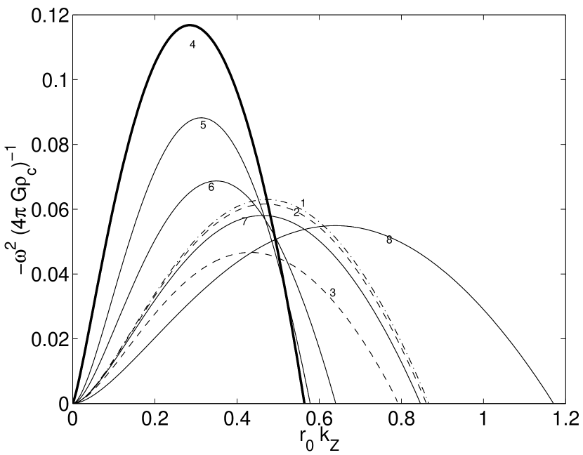
Figure 1: We have computed dispersion curves for truncated, unmagnetized, isothermal filaments. The external medium has finite density and a velocity dispersion of $\sigma_{e}=5\sigma$ for the solid curves. The curve shown as dot-dashed has an infinitely hot, zero density, external medium. The dashed curves have been computed using external media with velocity dispersions $\sigma_{e}=10\sigma$ for the upper curve, and $\sigma_{e}=2.5\sigma$ for the lower curve. Table 1 summarizes the results shown here.

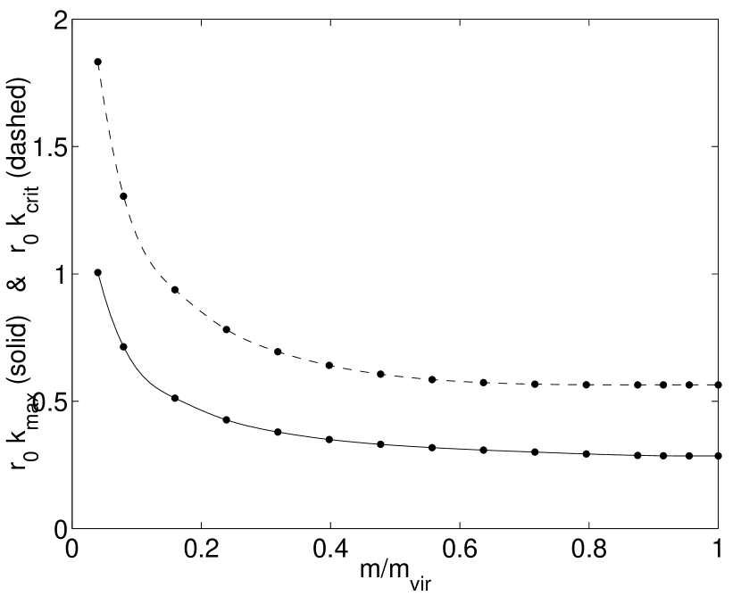
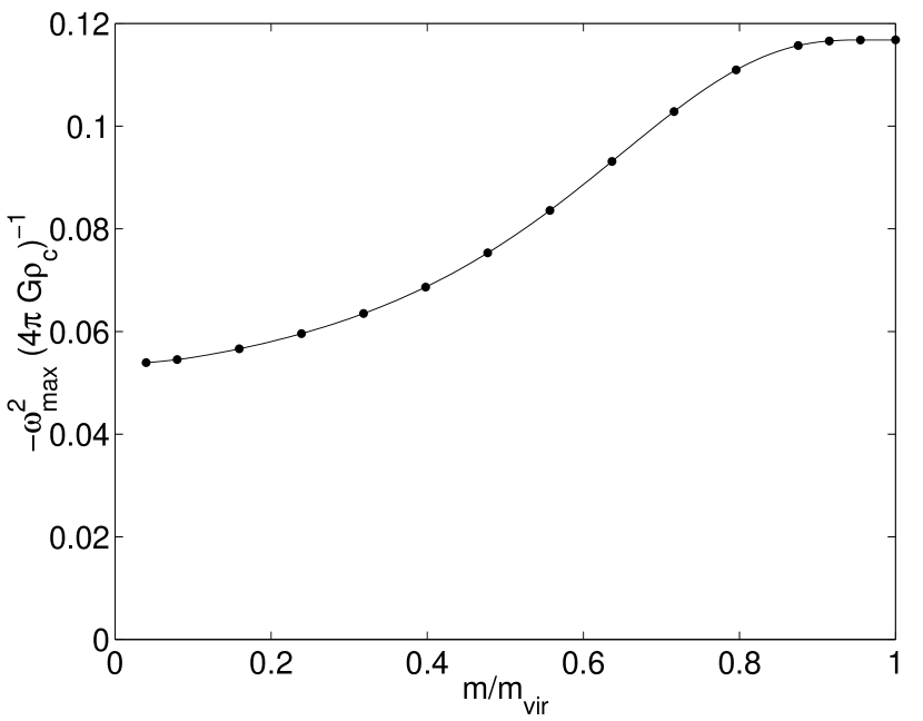
Figure 2: We plot the wave numbers $k_{z,max}$ and $k_{z,crit}$, as well as the squared growth rate $-\omega^{2}$ of the most unstable mode, as a function of the $m/m_{vir}$.

	$m/m_{vir}$	$P_{S}/\langle P\rangle$	C	$\tilde{k}_{z,max}$	$-\tilde{\omega}_{max}^{2}$	$\tilde{k}_{z,crit}$
1	0.199	0.801	0.472	0.149	0.063	0.866
2	0.199	0.801	0.47	0.149	0.0616	0.861
3	0.199	0.801	0.432	0.149	0.0467	0.791
4	1	0	$\infty$	0.285	0.117	0.564
5	0.597	0.403	0.537	0.313	0.0882	0.578
6	0.398	0.602	0.362	0.35	0.0687	0.64
7	0.199	0.801	0.149	0.462	0.0581	0.847
8	0.0995	0.901	-0.027	0.639	0.0549	1.17

Table 1: We give the the wave numbers and growth rates for the fastest growing modes of truncated, unmagnetized filaments (See Figure 1). We also give the critical growth rate, beyond which the filament is stable against axisymmetric perturbations. The tildes indicate dimensionless variables, as defined by equations 20. The external medium has finite density and a velocity dispersion of $\sigma_{e}=5\sigma$, except where otherwise indicated in the footnotes.

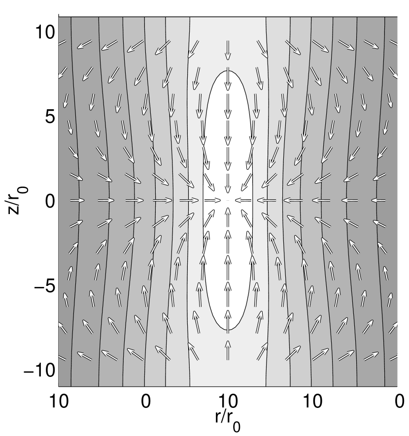
Figure 3: We show the eigenmode corresponding to the most unstable mode of the untruncated Ostriker solution ($r_{0}k_{z,max}=0.285$, $-\omega^{2}(4\pi G\rho_{c})^{-1}=0.117$). The contours show the density, while the arrows show the velocity field. We note that the segment shown is just one wavelength in the periodically fragmenting filament. The arrows are scaled logarithmically with the velocity, as discussed in the text.

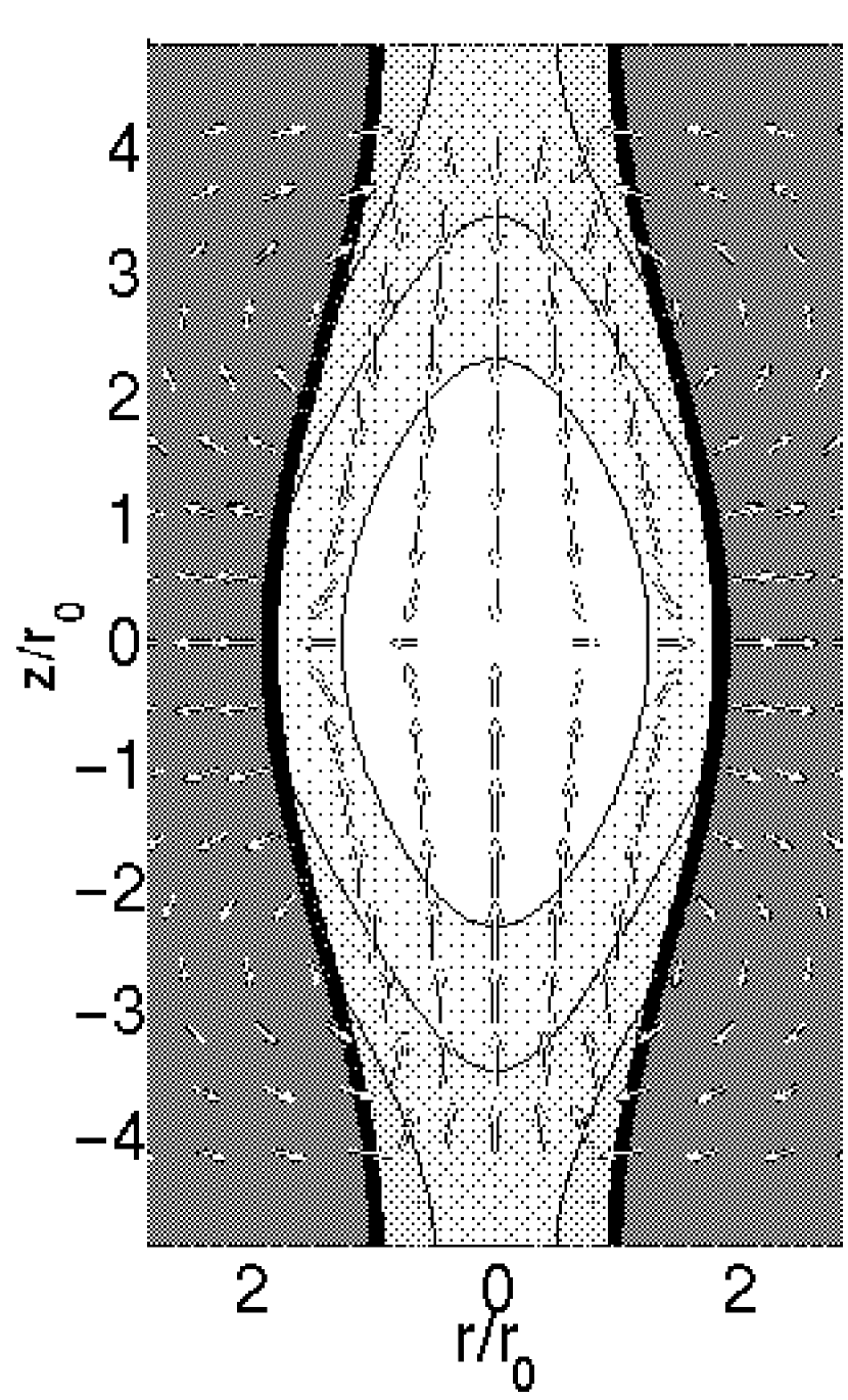
Figure 4: We show the eigenmode corresponding to the most unstable mode of a truncated Ostriker model with mass per unit length $m/m_{0}=5$ ($m/m_{vir}=0.199$). For this mode, $r_{0}k_{z,max}=0.462$ and $-\omega^{2}(4\pi G\rho_{c})^{-1}=0.449$.

Figure 2 shows how the mass per unit length affects the wave number $k_{z,max}$ and growth rate $-\omega_{max}^{2}$ of the most unstable mode, as well as the critical wave number $k_{z,crit}$. We find that the growth rate is significantly suppressed when $m/m_{vir}\stackrel{{\scriptstyle<}}{{\sim}}0.8$. The wave numbers remain essentially constant until $m/m_{vir}\approx 0.3$. For smaller masses per unit length, the wave number increases, corresponding to fragmentation on smaller length scales.

Two examples of eigenmodes are shown in figures 3 and 4 for unmagnetized filaments; the first shows the fragmentation of the untruncated Ostriker solution, while the second is significantly truncated ($m/m_{vir}=0.199$). These figures show a single wavelength in the periodic fragmentation of a filament. We note that the size of the perturbation is greatly exaggerated in these figures, where we typically add a perturbation of $\approx 33\%$ (in peak density) to the unperturbed solution.

The arrows in figures 3 and 4 show the velocity field, but the scaling is logarithmic due to the large range of velocities that must be shown. Specifically, $arrow~{}length\propto log_{10}(1+\alpha v/\sigma_{c})$, where we choose $\alpha\approx 50$. Both cases have purely poloidal velocity fields. The untruncated case shows an asymmetric infall onto the fragment, with almost purely radial infall near the fragments, and some radially outward motions between them. On the other hand, the truncated model shows infall along the axis, but the motions are actually radially outward in the vicinity of the fragment. This is due simply to the outward bulging of the fragment, which can occur because there is no infalling material approaching from the radial direction.

There are interesting motions in the gas outside of the truncated filament shown in Figure 4. We observe inward motions, that are driven by external pressure crushing the less dense parts of the filament between fragments. At the same time, the bulging of the filament near the fragments drives a radially outward flow in the surrounding gas. We emphasize that no mass is actually exchanged between the molecular filament and the surrounding atomic gas. Gas flows towards the fragments along the filament axis, which then bulge outwards slightly. This induces circulation motions in the surrounding envelope in which gas flows away from the fragments and towards the increasingly evacuated inter-fragment regions.

8 Stability of Truncated Filaments with Purely Poloidal and Purely Toroidal Fields

Following Paper I, we study the effects of poloidal and toroidal fields separately before considering the more general case of helical fields in Section 9. We note that none of the equilibrium models used in this Section fall within the range of observationally allowed models from Paper I. These models are useful, however, in that they provide insight into the roles played by the field components in more general helical field models.

8.1 Poloidal Field Results

Figure 5 shows a sequence of dispersion curves, in which we have varied the poloidal flux to mass ratio $\Gamma_{z}$ while holding the mass per unit length constant at $m=5~{}m_{0}$ ($m/m_{vir}=0.199$). We observe that the poloidal field has a stabilizing effect on the filament, but that the stabilization saturates for $\Gamma_{z}\stackrel{{\scriptstyle>}}{{\sim}}10$. The critical and most unstable wave numbers are decreased by the poloidal field, but this effect also saturates when $\Gamma_{z}\stackrel{{\scriptstyle>}}{{\sim}}10$. These results agree qualitatively with those obtained by Nagasawa (1987) for pressure truncated isothermal filaments threaded by purely poloidal fields, although the degree of stabilization is greater in our model. Chandrasekhar and Fermi (1953) also find that poloidal fields stabilize incompressible filaments, but they do not find any saturation of the stabilizing effect. This is especially apparent in Figure 6, where we have plotted $k_{z,max}$, $k_{z,crit}$, and $-\omega_{max}^{2}$ as a funtion of $\Gamma_{z}$.

Figures 7 and 8 show two eigenmodes corresponding, respectively, to a weak ($\Gamma_{z}=1$) and relatively strong ($\Gamma_{z}=5$) poloidal field. Naturally, as the poloidal flux to mass ratio increases, and the field strengthens, the gas becomes more tightly constrained to move only along the field lines. When $\Gamma_{z}\stackrel{{\scriptstyle>}}{{\sim}}10$, the motions are almost entirely poloidal; further increasing $\Gamma_{z}$ has no significant effect on the motions, and, hence, no significant effect on the dispersion curves.

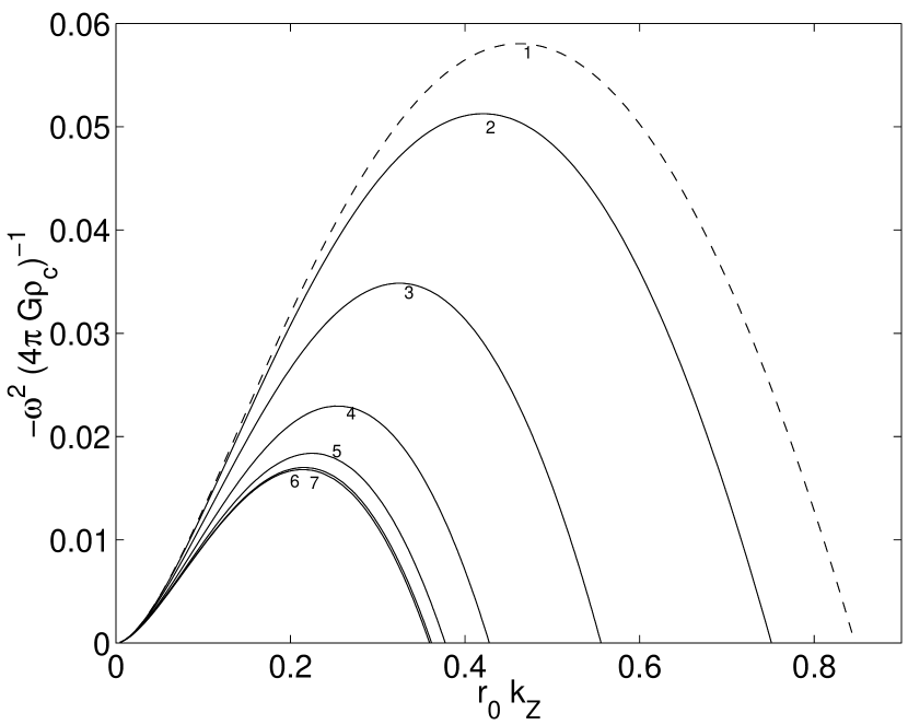
Figure 5: We have computed dispersion curves for truncated filaments with poloidal field only. In all cases, the mass per unit length is $5m_{0}$ ($m/m_{vir}=0.199$), which falls within the range of observationally allowed masses per unit length found in Paper I. We have also assumed an external medium which is perfectly conducting and of finite density, with $\sigma_{e}=5\sigma$. The labeling of the dispersion curves corresponds to the numbering in Table 2.

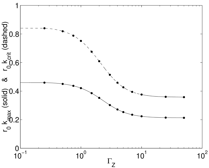
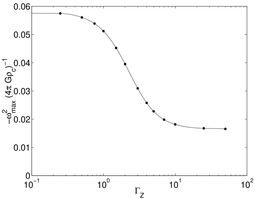
Figure 6: We plot the wave numbers $k_{z,max}$ and $k_{z,crit}$, as well as the squared growth rate $-\omega^{2}$ of the most unstable mode, as a function of the $\Gamma_{z}$.

	$\Gamma_{z}$	C	$P_{S}/\langle P\rangle$	$\tilde{k}_{z,max}$	$-\tilde{\omega}_{max}^{2}$	$\tilde{k}_{z,crit}$
1	0	0.149	0.801	0.462	0.0581	0.846
2	1	0.146	0.813	0.421	0.0513	0.751
3	2.5	0.133	0.859	0.325	0.0348	0.556
4	5	0.116	0.929	0.254	0.023	0.428
5	10	0.106	0.977	0.225	0.0184	0.377
6	25	0.102	0.996	0.216	0.017	0.362
7	50	0.101	0.999	0.214	0.0168	0.359

Table 2: We give the the wave numbers and growth rates for the fastest growing modes of truncated filaments with poloidal field only (See Figure 5). We also give the critical growth rate, beyond which the filament is stable against axisymmetric perturbations. In all cases, the mass per unit length is $5m_{0}$ ($m/m_{vir}=0.199$), which falls within the range of observationally allowed masses per unit length found in Paper I. We have also assumed an external medium which is perfectly conducting and of finite density, with $\sigma_{e}=5\sigma$.

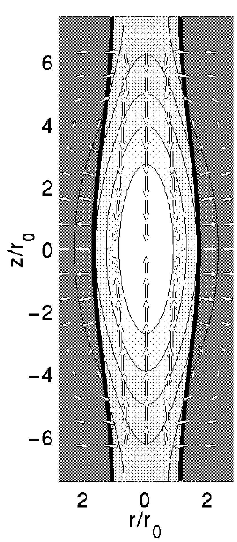
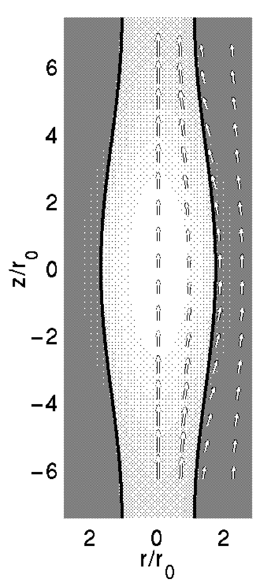
Figure 7: We show the eigenmode corresponding to the most unstable mode of a truncated magnetized model with a weak poloidal field ($\Gamma_{z}=1$), and mass per unit length $m/m_{0}=5$ ($m/m_{vir}=0.199$). For this mode, $r_{0}k_{z,max}=0.421$ and $-\omega^{2}(4\pi G\rho_{c})^{-1}=0.0512$. The figures represent a) (left panel) density contours with superimposed poloidal velocity vectors. We note that there is no toroidal velocity when the field is purely poloidal. and b) (right panel) The magnetic field. We always represent the magnetic field as a split-frame figure, with poloidal field vectors shown on the right, and contours to represent the toroidal field on the left. Since no toroidal field is generated in this case, the left side of the figure is left blank.

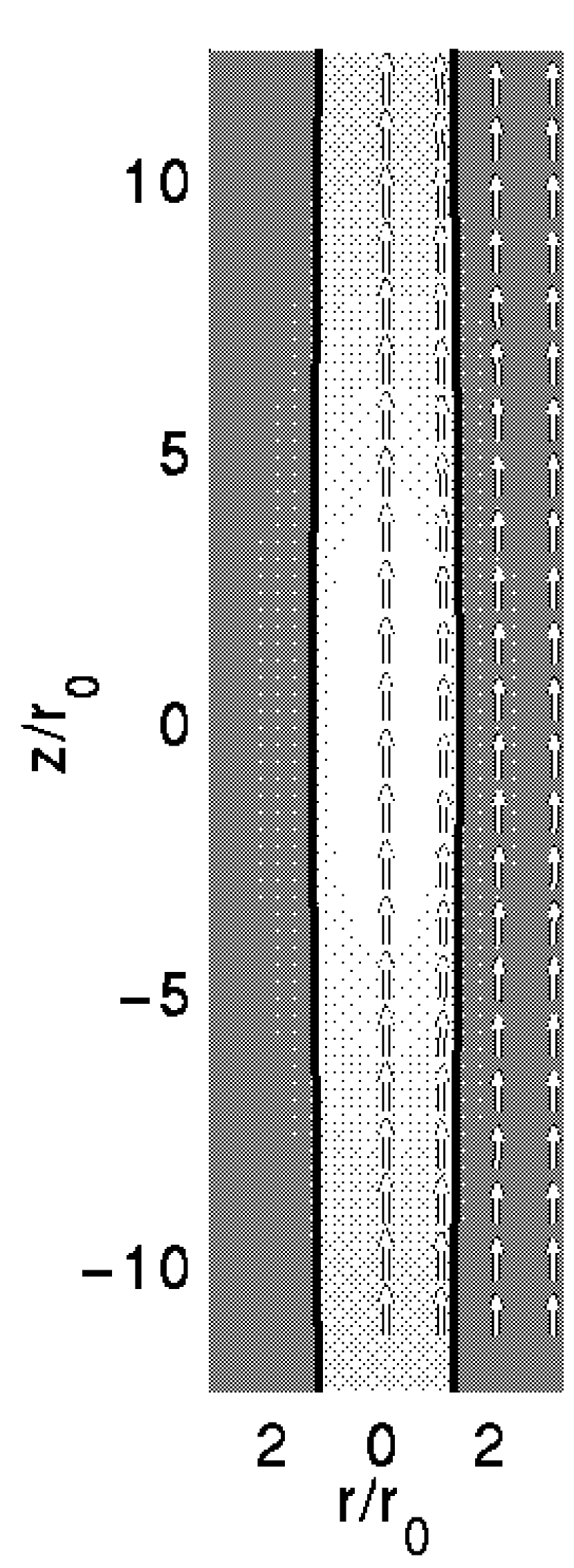
Figure 8: We show the eigenmode corresponding to the most unstable mode of a truncated magnetized model with a relatively strong poloidal field ($\Gamma_{z}=5$), and mass per unit length $m/m_{0}=5$ ($m/m_{vir}=0.199$). For this mode, $r_{0}k_{z,max}=0.225$ and $-\omega^{2}(4\pi G\rho_{c})^{-1}=0.0228$. The figures represent a) (left panel) density contours with superimposed poloidal velocity vectors. We note that there is no toroidal velocity when the field is purely poloidal. and b) (right panel) The magnetic field. We always represent the magnetic field as a split-frame figure, with poloidal field vectors shown on the right, and contours to represent the toroidal field on the left. Since no toroidal field is generated in this case, the left side of the figure is left blank.

8.2 Toroidal Field Results

Finally we consider models in which the magnetic field is purely toroidal. We stress that these models are illustrative only, and certainly do not represent realistic models of filamentary clouds. Figure 9 shows a sequence of dispersion curves, in which we have varied the toroidal flux to mass ratio $\Gamma_{\phi}$ while holding the mass per unit length constant at $m=5~{}m_{0}$ ($m/m_{vir}=0.199$). We observe that the toroidal field strongly stabilizes the cloud against fragmentation. Contrary to the effects of the poloidal field, the stabilization does not saturate; in fact, the models are completely stable against fragmentation when $\Gamma_{\phi}\stackrel{{\scriptstyle>}}{{\sim}}10$. Purely toroidal fields have a stabilizing effect because fragmentation requires a flow of material along the axis of the filament, which must result in substantial compression of the toroidal flux tubes. This results in a gradient in the magnetic pressure $1/8\pi~{}\partial B_{\phi}^{2}/\partial z$ which resists this motion. When the toroidal flux to mass ratio $\Gamma_{\phi}$ is sufficiently high, the toroidal flux tubes can resist compression and arrest fragmentation altogether. The effects of the varying $\Gamma_{\phi}$ are most readily apparent in Figure 10, where we have plotted $k_{z,max}$, $k_{z,crit}$, and $-\omega_{max}^{2}$ as a function of of $\Gamma_{\phi}$. We have shown an example of an eigenmode in figures 11, where $\Gamma_{\phi}=5$. In both cases, the toroidal field becomes strongest near the fragments. The gas motions are purely poloidal in both cases, with a “reverse flow” just outside of the filament. As in the purely hydrodynamic case, the gas is pushed radially outward near the fragment, and flows toward the empty regions between them. However, the pinch of the toroidal field restricts the motions to a narrow band just outside the filament.

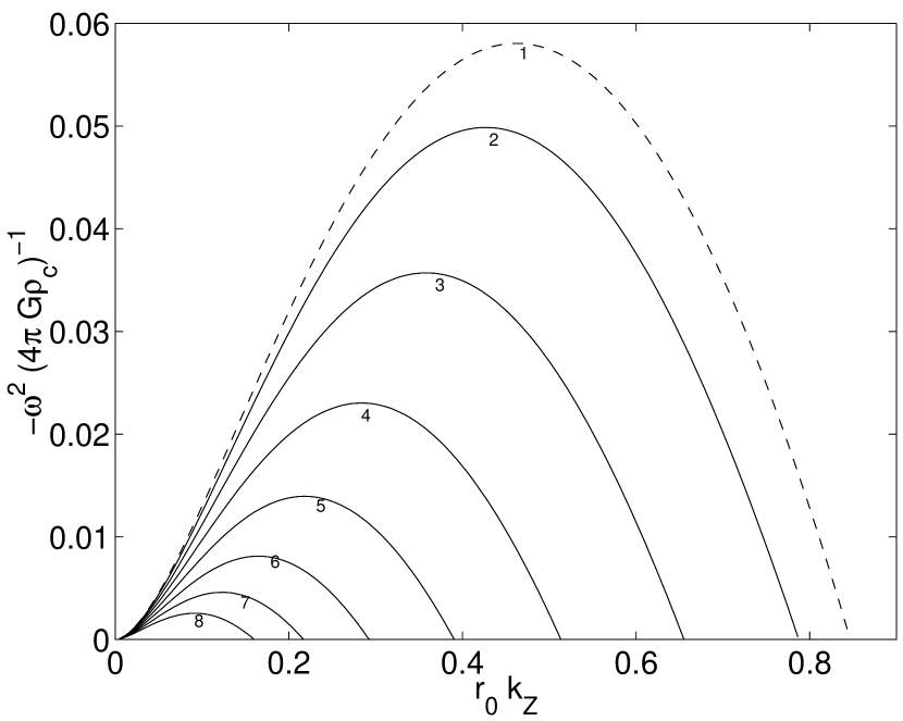
Figure 9: We have computed dispersion curves for truncated filaments with toroidal field only. In all cases, the mass per unit length is $5m_{0}$ ($m/m_{vir}=0.199$), which falls within the range of observationally allowed masses per unit length found in Paper I. We have also assumed an external medium which is perfectly conducting and of finite density, with $\sigma_{e}=5\sigma$. The labeling of the dispersion curves corresponds to the numbering in Table 3.

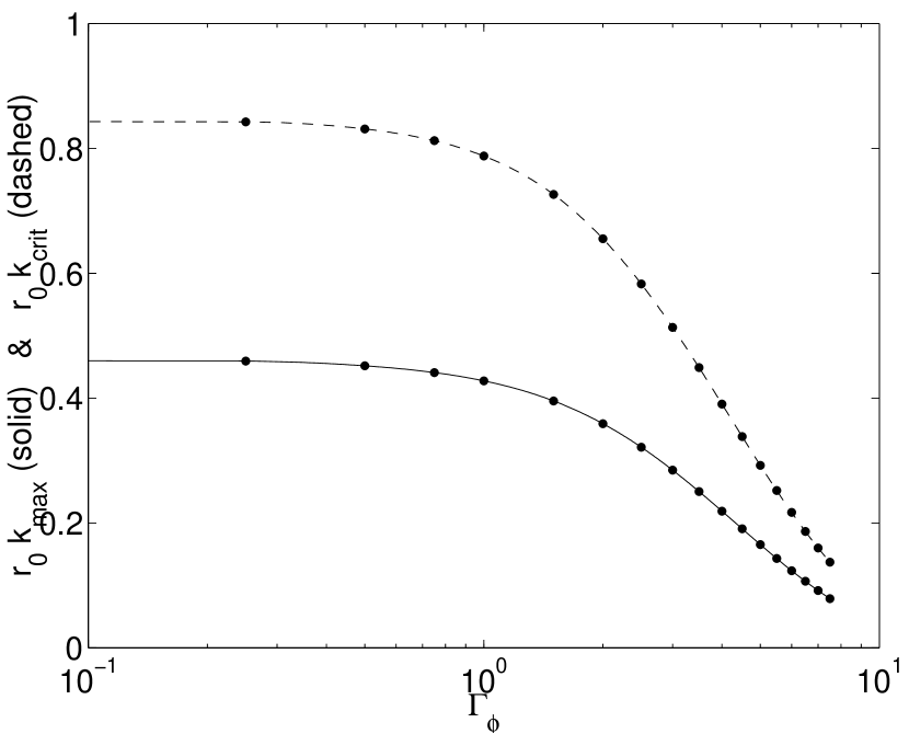
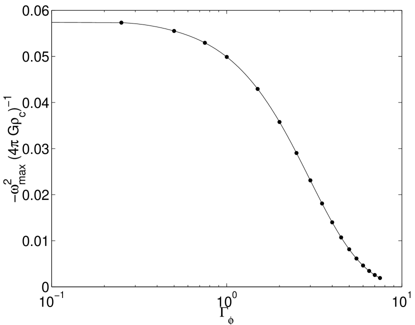
Figure 10: We plot the wave numbers $k_{z,max}$ and $k_{z,crit}$, as well as the squared growth rate $-\omega^{2}$ of the most unstable mode, as a function of the $\Gamma_{\phi}$.

	$\Gamma_{\phi}$	C	$P_{S}/\langle P\rangle$	$\tilde{k}_{z,max}$	$-\tilde{\omega}_{max}^{2}$	$\tilde{k}_{z,crit}$
1	0	0.149	0.801	0.462	0.0581	0.846
2	1	0.162	0.764	0.427	0.0499	0.787
3	2	0.199	0.683	0.358	0.0357	0.655
4	3	0.253	0.598	0.284	0.023	0.513
5	4	0.318	0.523	0.218	0.0139	0.39
6	5	0.392	0.462	0.165	0.00811	0.293
7	6	0.471	0.413	0.123	0.0046	0.217
8	7	0.555	0.372	0.0914	0.00256	0.16

Table 3: We give the the wave numbers and growth rates for the fastest growing modes of truncated filaments with toroidal field only (See Figure 9). We also give the critical growth rate, beyond which the filament is stable against axisymmetric perturbations. In all cases, the mass per unit length is $5m_{0}$ ($m/m_{vir}=0.199$), which falls within the range of observationally allowed masses per unit length found in Paper I. We have also assumed an external medium which is perfectly conducting and of finite density, with $\sigma_{e}=5\sigma$.

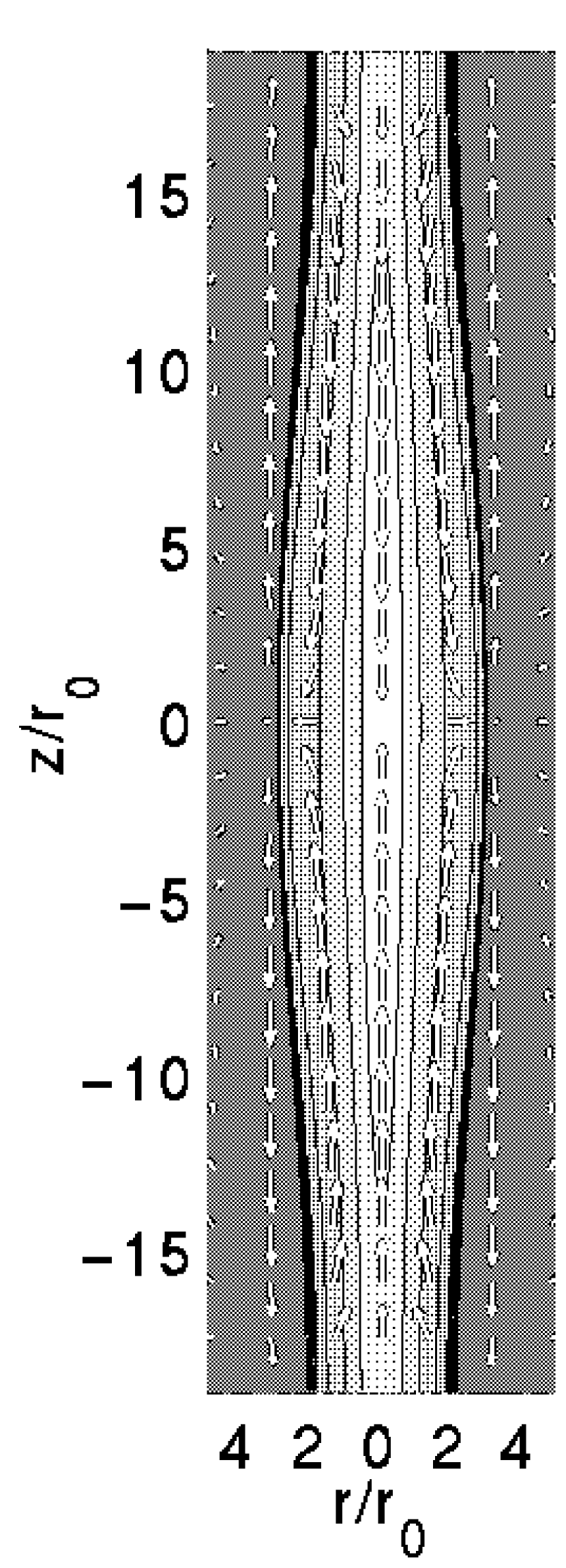
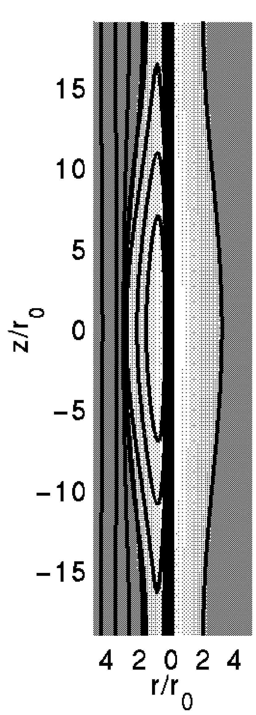
Figure 11: We show the eigenmode corresponding to the most unstable mode of a truncated magnetized model with a toroidal field ($\Gamma_{\phi}=5$), and mass per unit length $m/m_{0}=5$ ($m/m_{vir}=0.199$). For this mode, $k_{z,max}=0.165$ and $-\omega^{2}(4\pi G\rho_{c})^{-1}=0.0081$. The figures represent a) (left panel) density contours with superimposed poloidal velocity vectors. We note that there is no toroidal velocity when the field is purely toroidal. and b) (right panel) The magnetic field. We always represent the magnetic field as a split-frame figure, with poloidal field vectors shown on the right, and contours to represent the toroidal field on the left. Since no poloidal field is generated in this case, the right side of the figure is left blank.

9 Stability of Filamentary Clouds With Helical Magnetic Fields

In this Section, we consider the stability of models that best agree with the observational constraints found in Paper I:

$$0.11\leq\frac{m}{m_{vir}}\leq 0.43$$

$$0.012\leq\frac{P_{S}}{\langle P\rangle}\leq 0.75.$$

$$0.2\leq X\leq 5,$$ (23)

(24)

where the reader is refered to Paper I for a description of the various quantities. We used a Monte Carlo exploration of our three dimensional ($\Gamma_{z}$, $\Gamma_{\phi}$, and $C$) parameter space to find a set of models that agree with these constraints. We use the same set of models here to determine the stability properties of filamentary clouds threaded by helical fields. It is not necessary to show full dispersion curves for all models, since most of the useful information is contained in the dispersion parameters $k_{z,max}$, $k_{z,crit}$, and $-\omega_{max}^{2}$. Thus, we try to determine which combination of model parameters $\Gamma_{z}$, $\Gamma_{\phi}$, and $C$   controls the stability properties.

We find that the dispersion parameters $k_{z,max}$, $k_{z,crit}$, and $-\omega_{max}^{2}$ are best correlated with the ratio $\Gamma_{\phi}/\Gamma_{z}$. Figures 12 to 14 show scatter plots of these dispersion parameters as functions of $\Gamma_{\phi}/\Gamma_{z}$. It is obvious from these figures that we have found two types of unstable mode in our calculation; the two types of unstable mode are mostly well separated in Figures 12 to 14, but join together when $\Gamma_{\phi}/\Gamma_{z}\approx 2$. The first, which occurs when $\Gamma_{\phi}/\Gamma_{z}$ is small, is a gravity-driven instability, which is analogous to the modes found for purely hydrodynamic models (Section 7), and MHD models in which the field is purely poloidal or toroidal (Section 8). We note that increasing $\Gamma_{\phi}/\Gamma_{z}$ substantially decreases the growth rate of the instability. This is in accord with the findings of Section 8, where we found that increasing $\Gamma_{\phi}$ and $\Gamma_{z}$ both stabilize gravity driven modes, but $\Gamma_{\phi}$ is much more effective. In fact, virtually all of the gravity-driven modes in Figure 13 have growth rates that are significantly lower than the growth rates of unmagnetized filaments, as well as filaments with purely poloidal fields (shown in figures 1 and 5 respectively). Typically, we find

$$0.0005 \stackrel{{\scriptstyle<}}{{\sim}} -{\tilde{\omega}}_{max}^{2}\stackrel{{\scriptstyle<}}{{\sim}}0.03$$

$$0.1 \stackrel{{\scriptstyle<}}{{\sim}} \tilde{k}_{z,max}\stackrel{{\scriptstyle<}}{{\sim}}0.3$$

$$0.2 \stackrel{{\scriptstyle<}}{{\sim}} \tilde{k}_{z,crit}\stackrel{{\scriptstyle<}}{{\sim}}0.6,$$ (25)

where the tildes refers to the dimensionless growth rates and wave numbers, as defined in equation 20.

By taking the inverse of $\sqrt{-\omega^{2}}$, we find a growth timescale of

$$\tau_{frag}=1.8\left(\frac{-\tilde{\omega}_{max}^{2}}{0.01}\right)^{-1/2}\left(\frac{n_{c}}{10^{4}~{}cm^{-3}}\right)^{-1/2}~{}Myr.$$ (26)

where $n_{c}$ is the central number density of the filament. We have chosen a fiducial central density of $10^{4}~{}cm^{-3}$ because radially extended ($0.5~{}pc$ diameter) filamentary structure is clearly visible in $C^{18}O$ maps of Taurus (Onishi et al. 1998). $C^{18}O$ molecules require a density of at least $\sim 2\times 10^{3}~{}cm^{-3}$ for excitation, and our models predict that the central density should be several times higher than the bulk of the filament. Nevertheless, the central densities of filaments have not yet been accurately measured, so this fiducial central density should be treated with caution. The radial signal crossing time is approximately given by

$$\tau_{x}\approx\frac{Rs}{\sigma}=0.49\left(\frac{R_{S}}{0.25~{}pc}\right)\left(\frac{0.5~{}km~{}s^{-1}}{\sigma}\right)~{}Myr.$$ (27)

Since the signal crossing time is comparable to, and probably slightly longer than the fragmentation timescale, we expect filamentary clouds to achieve radial quasi-equilibrium before fragmentation destroys the filament in a few times $\tau_{frag}$; thus, our analysis is consistent with the assumption of quasi-equilibrium used in Paper I.

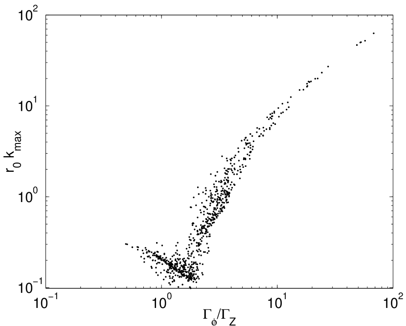
Figure 12: The most unstable wave numbers for a random sample of models that agree with our constraints.

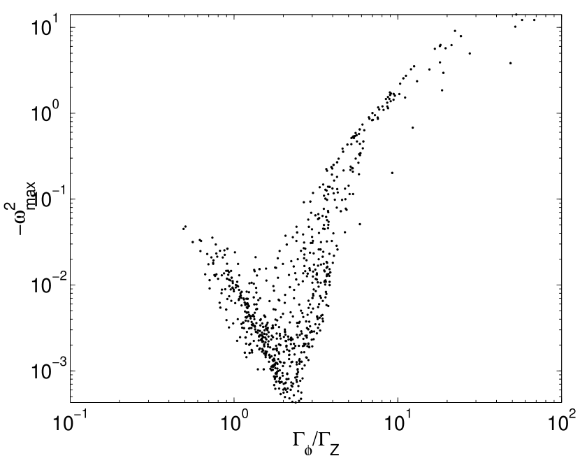
Figure 13: The growth rates for a random sample of models that agree with our constraints.

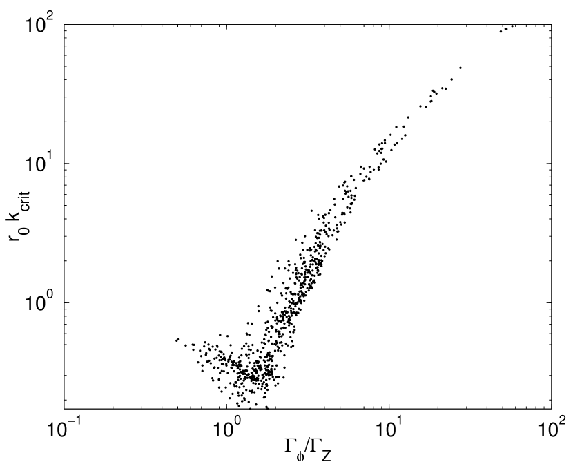
Figure 14: The critical wave numbers for a random sample of models that agree with our constraints.

The second type of unstable mode is driven by the magnetic field. These MHD-driven instabilities are triggered when $\Gamma_{\phi}/\Gamma_{z}\stackrel{{\scriptstyle>}}{{\sim}}2$. Figures 12 to 14 show that this mode joins onto the gravity-driven modes, but extends to very high growth rates and very large wave numbers. Since large wave numbers correspond to small wavelengths, gravity cannot be important, as a driving force, for these modes. They are, however, most unstable when the toroidal flux wrapping the filament is large, compared to the poloidal flux. This suggests that the mode is an MHD instability. In fact the criterion that we have found is analogous to the famous stability criterion for MHD “sausage” modes:

$$B_{\phi S}>\sqrt{2}B_{z}$$ (28)

(cf. Jackson 1975). The analogy is far from perfect because equation 28 applies to the case of a uniform plasma cylinder threaded by a constant poloidal magnetic field, and surrounded by a toroidal field driven by a thin axial current sheet along the surface of the plasma. However, the axial current distribution in our case is distributed throughout the filament. Nevertheless, the similarity between equation 28 and our own instability criterion is very suggestive.

We do not find MHD-driven instabilities for models with purely toroidal fields. We note that the stability criterion for a non-self-gravitating plasma column pinched by a purely toroidal field can be expressed analytically as

$$-\frac{d\ln P}{d\ln r}<\frac{4}{2+\beta}$$ (29)

for an isothermal perturbation, where $\beta$ is the usual plasma $\beta$, defined by $\beta=8\pi P/B_{\phi}^{2}$ (cf. Sitenko & Malnev 1995). We have checked, numerically, that our equilibria obey equation 29, and, therefore, should be stable against “sausage” modes. It may appear that equation 28 is violated for any model with a purely toroidal field, but we remind the reader that equation 28 strictly applies to situations in which the toroidal field is generated by a current sheet at the plasma surface, and thus resides entirely outside of the plasma column. Equation 29 is, however, appropriate for the more distributed fields in our models.

It seems paradoxical that models with purely toroidal fields are stable against “sausage” modes, while those with a poloidal field component may be unstable. However, we note that helical fields are topologically different from purely toroidal fields. Flux tubes in purely toroidal models form closed loops, while the loops of toroidal flux are all linked in the case of a helical field. When the field is helical, twisting motions in the filament may enhance the toroidal field, while no amount of twisting can amplify a purely toroidal field. Thus, we argue that it is at least possible for modes to exist that simultaneously generate twisting motions and toroidal field, which could destabilize the filament.

We note that the gravity-driven modes join continuously with the MHD-driven modes in Figures 12 to 14; the intersection of the two branches, when $\Gamma_{\phi}/\Gamma_{z}\approx 2$, represents a transition between gravity and the toroidally dominated magnetic field as the main driving force of the instabilty. Some of the modes that we have labeled as magnetic have growth rates that are similar to gravity modes, except that the wavelength is somewhat shorter. These may represent reasonable modes of fragmentation for filamentary clouds. However, the more unstable modes of the MHD branch probably cannot, since they grow too rapidly and would probably disrupt the filament on timescales that are much shorter than the timescale on which equilibrium can be established (See equations 26 and 27). Therefore, a subset of the models allowed by the observational constraints of FP1 are actually highly unstable.

In Figure 15, we show an example of an unstable gravity-driven mode. As in the previously considered cases of hydrodynamic filaments (Section 7) and filaments with only one field component (Section 8), gravity drives a purely poloidal flow of gas towards the fragments. However, a helical field results in a toroidal component of the velocity field which alternates in sign from one side of the fragment to the other. The reason is that the helical field exerts oppositely directed torques on the gas flowing towards the fragment from opposite directions. The mode shown in Figure 16 is driven by the MHD “sausage” instability. The dominant wavelength of the instability is much shorter than either the filament radius or the dominant wavelength of the gravity-driven modes; therefore gravity is relatively unimportant compared to the magnetic stresses. The actual structure of the mode is quite similar to that of the gravity-driven modes except that the mode is confined to the most central parts of the filament, where the $B_{\phi}$ gradient is steepest. This is consistent with our claim that this mode is a “sausage” instability, because “sausage” modes are driven by outwardly increasing toroidal fields with strong gradients. The filament is crushed where the toroidal field is strongest, which forces gas out along the axis and towards the fragments. As in the case of the gravity-driven modes, toroidal motions are generated as the helical field exerts torques on the gas.

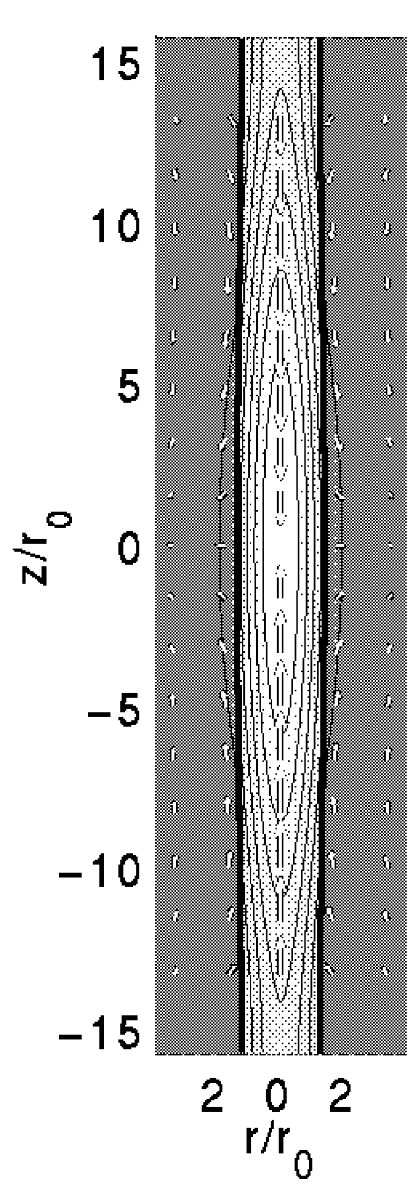
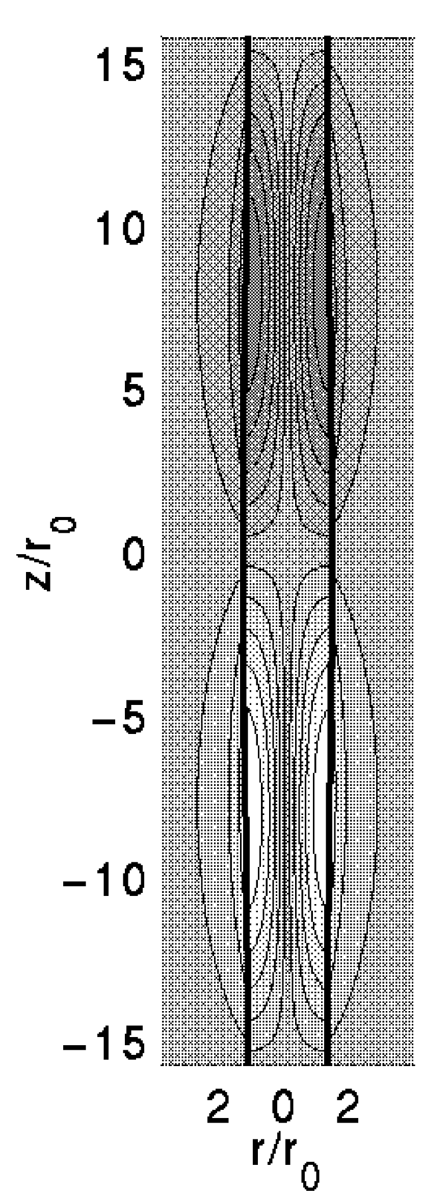
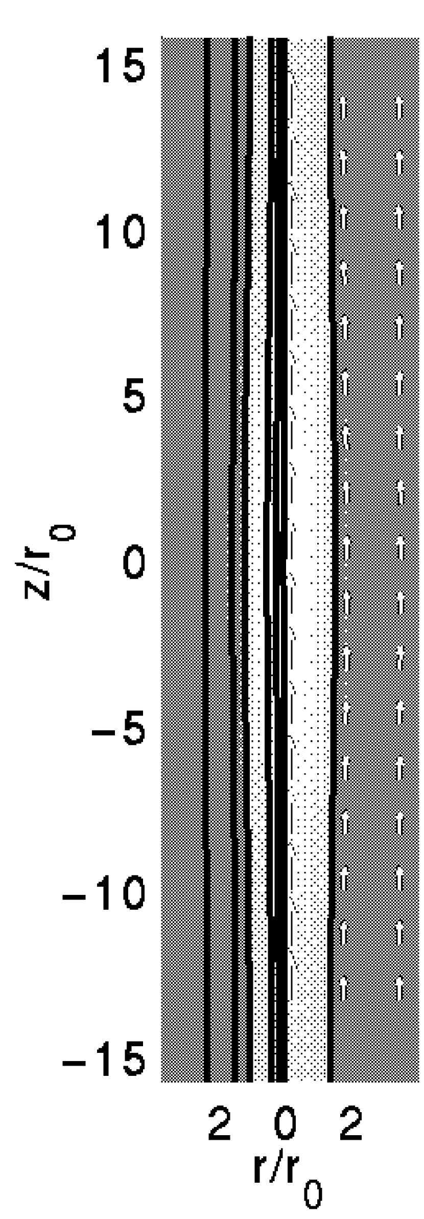
Figure 15: An example of a gravity-driven mode for a model with a helical magnetic field. For this mode, $k_{z,max}=0.199$ and $-\omega^{2}(4\pi G\rho_{c})^{-1}=0.0081$. The figures represent a) (left panel) density contours with superimposed poloidal velocity vectors. b) (middle panel) Contours of toroidal velocity. Light coloured contours represent positive $v_{\phi}$, while dark coloured contours represent negative $v_{\phi}$. and c) (right panel) The magnetic field. We always represent the magnetic field as a split-frame figure, with poloidal field vectors shown on the right, and contours to represent the toroidal field on the left.

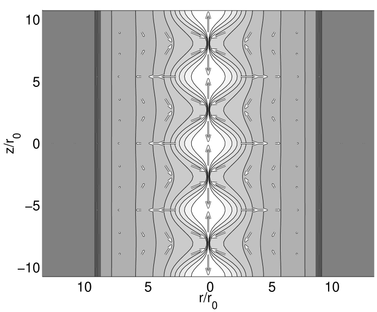
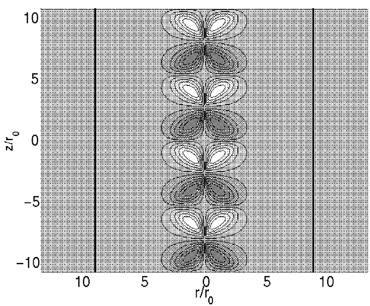
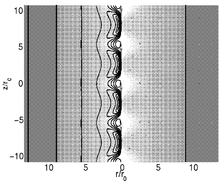
Figure 16: An example of an MHD-driven mode for a model with a helical magnetic field. For this mode, $k_{z,max}=1.17$ and $-\omega^{2}(4\pi G\rho_{c})^{-1}=0.0390$. The figures represent a) (top panel) density contours with superimposed poloidal velocity vectors. b) (middle panel) Contours of toroidal velocity. Light coloured contours represent positive $v_{\phi}$, while dark coloured contours represent negative $v_{\phi}$. and c) (bottom panel) The magnetic field. We always represent the magnetic field as a split-frame figure, with poloidal field vectors shown on the right, and contours to represent the toroidal field on the left.

Figure 17 shows the effect of $\Gamma_{\phi}/\Gamma_{z}$ on the ratio of the fragmentation wavelength $\lambda_{max}$ to the filament diameter $D$, which we define as twice the filament radius $R_{S}$; we note that gravity-driven and MHD-driven modes cannot be easily separated on this diagram. In all cases, we find that more toroidally dominated modes have smaller $\lambda_{max}/D$. The Schneider and Elmegreen (1979) Catalogue of Dark Globular Filaments shows that $\lambda_{max}/D\approx 3.0$ for most filaments in their sample. Interestingly, this value is consistent with $\Gamma_{\phi}/\Gamma_{z}\approx 2$, which is near the transition from gravity to MHD-driven modes, and is near the lowest possible growth rate. We postulate that most filamentary clouds may be observed to reside near this maximally stable configuration because such objects would survive the longest. Although suggestive, this conclusion will also depend on the non-axisymmetric stability of filamentary clouds, to be discussed in a forthcoming paper.

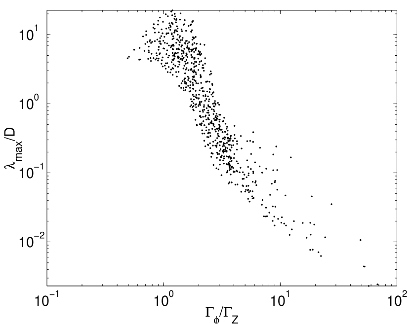
Figure 17: The ratio of fragment separation $\lambda_{max}=2\pi/k_{max}$ to filament diameter $D=2R_{S}$ for a random sample of models that agree with our constraints.

Finally, in Figure 18, we show the masses of fragments that might form from filamentary clouds. We note that we have computed the fragment masses simply by multiplying the equilibrium mass per unit length by the wavelength of the most unstable mode. This procedure implicitly assumes that there is no sub-fragmentation as fragments evolve. Thus, these masses should be regarded with caution. We find that fragment masses, computed in this way, fall in a rather large range; in dimensionless units we find

$$100\stackrel{{\scriptstyle<}}{{\sim}}M_{frag}(4\pi G)^{3/2}\rho_{c}^{1/2}\sigma^{-3}\stackrel{{\scriptstyle<}}{{\sim}}400$$ (30)

for gravity-driven modes, which have $\Gamma_{\phi}/\Gamma_{z}\stackrel{{\scriptstyle<}}{{\sim}}2$. Thus, we obtain masses of

$$M_{frag}=41.5\left(\frac{\tilde{M}_{frag}}{100}\right)\left(\frac{\sigma}{0.5km~{}s^{-1}}\right)^{3}\left(\frac{n_{c}}{10^{4}~{}cm^{-3}}\right)^{-1/2}M_{\odot}.$$ (31)

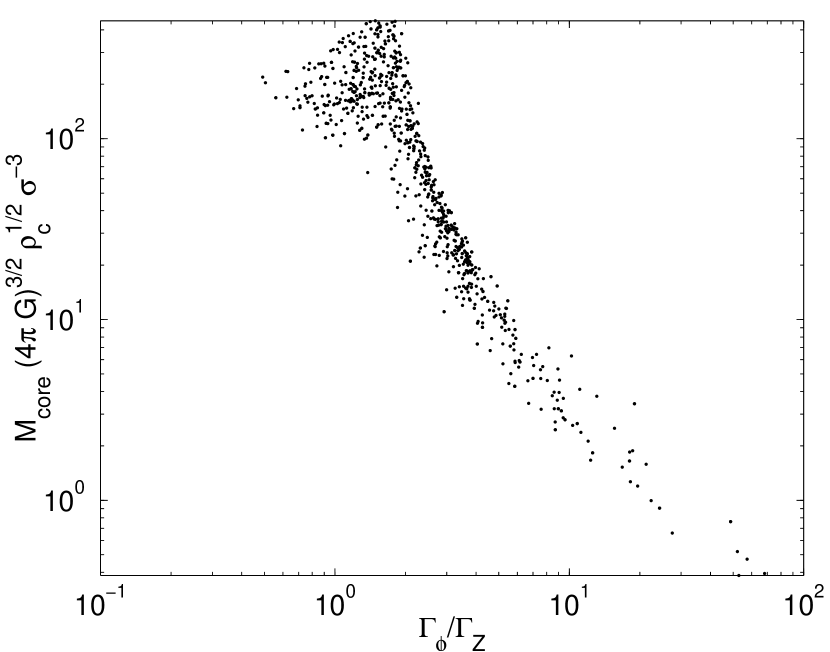
Figure 18: The expected mass of fragments for a random sample of models that agree with our constraints. Here we assume that $M_{frag}=m\lambda_{max}$.

10 Discussion and Summary

We have determined how pressure truncation and helical fields affect the stability of our models against axisymmetric modes of fragmentation, which are ultimately responsible for the formation of cores. Our analysis differs from previous work on filaments in a number of respects. Firstly, and most importantly, we have made at least a first attempt to obervationally constrain our models; thus, our modes of fragmentation pertain to equilibria that are truncated by realistic external pressures and have magnetic fields that are consistent with the observations. Moreover, our models have density gradients of $r^{-1.8}$ to $r^{-2}$, in good agreement with observational data (Alves et al 1998, Lada et al. 1998). Secondly, we have treated the external medium self-consistently by considering it to be a perfectly conducting gas of finite density.

We found, in Paper I, that filaments that are highly truncated by the external pressure have lower masses per unit length than untruncated filaments. We have shown, in Section 7, that such pressure dominated equilibria are more stable than their less truncated gravitationally dominated counterparts. We also found that the finite density of the external medium, in our calculation, slightly stabilizes filaments due to inertial effects. This effect vanishes when the external medium is “hot”, with a velocity dispersion $\stackrel{{\scriptstyle>}}{{\sim}}10~{}\sigma$.

Both the poloidal and toroidal fields were shown to stabilize filaments against gravity-driven fragmentation in Section 8. The poloidal field stabilizes the filament by resisting motions perpendicular to the poloidal field lines. This stabilization eventually saturates, when the field is strong enough ($\Gamma_{z}\stackrel{{\scriptstyle>}}{{\sim}}10$) to disallow radial motions altogether. Surprisingly, the toroidal field is much more effective at stabilizing filaments against gravitational fragmentation. As the filaments begins to fragment, the toroidal flux tubes are pushed together near the fragments; this results in a gradient in the magnetic pressure ($1/8\pi~{}\partial B_{phi}^{2}/\partial z$) that opposes fragmentation. In the unrealistic limit of purely toroidal fields, the filament is stable to fragmentation when $\Gamma_{\phi}\stackrel{{\scriptstyle>}}{{\sim}}7$. One might expect that these models would be highly unstable against MHD “sausage” modes. However, we have verified that our equilibria satisfy the stability condition given in equation 29.

In Section 9, we demonstrated that our models with helical fields are subject to both gravity-driven and MHD-driven instabilities. The two types of modes blend together in Figures 12 to 14, with the transition from gravity-driven to MHD-driven largely determined by the ratio $\Gamma_{\phi}/\Gamma_{z}$; when $\Gamma_{\phi}/\Gamma_{z}\stackrel{{\scriptstyle<}}{{\sim}}2$, the instability is driven by gravity, with MHD-driven modes triggered only for more tightly wrapped helical fields. We provided evidence, in Section 9, that the MHD-driven mode is probably is an MHD “sausage” mode. These instabilities can have extremely high growth rates compared to gravity driven modes; therefore, we may interpret our stability condition as an additional theoretical constraint on our models. We note that the most stable of all equilibria are near the transition from grivity-driven to MHD-driven modes. Thus, we find that there is a regime in which filamentary clouds fragment very slowly. For gravity-driven modes, we find that $-\omega_{max}^{2}$, $k_{z,max}$, and $k_{z,crit}$ fall within the ranges

$$0.0005 \stackrel{{\scriptstyle<}}{{\sim}} -\omega_{max}^{2}(4\pi G\rho_{c})^{-1}\stackrel{{\scriptstyle<}}{{\sim}}0.03$$

$$0.1 \stackrel{{\scriptstyle<}}{{\sim}} r_{0}k_{z,max}\stackrel{{\scriptstyle<}}{{\sim}}0.3$$

$$0.2 \stackrel{{\scriptstyle<}}{{\sim}} r_{0}k_{z,crit}\stackrel{{\scriptstyle<}}{{\sim}}0.6,$$ (32)

where $r_{0}$ is the core radius for filamentary clouds (see Paper I), and $\rho_{c}$ is the central density. We may also write the expected wavelength for the separation of fragments and the growth timesacale as

$$\lambda_{max} = 2.8\left(\frac{\tilde{k}_{max}}{0.2}\right)^{-1}\left(\frac{\sigma_{c}}{0.5~{}km~{}s^{-1}}\right)\left(\frac{n_{c}}{10^{4}~{}cm^{-3}}\right)^{-1/2}~{}pc$$

$$\tau_{frag} = 1.8\left(\frac{-\tilde{\omega}_{max}^{2}}{0.01}\right)^{-1/2}\left(\frac{n_{c}}{10^{4}~{}cm^{-3}}\right)^{-1/2}~{}Myr.$$ (33)

We note that the growth time for gravity-driven modes is much longer than the radial signal crossing time (equation 27), on which radial equilibrium is established. Therefore, our stability analysis is consistent with the assumption of radial quasi-equilibrium used in Paper I.

We find that the fragmentation of filamentary clouds with helical fields leads to a toroidal component of the velocity field, whose direction alternates with every half wavelength of the perturbation. These motions are comparable to, and in some cases exceed the poloidal velocities, at least in linear theory. These motions could, in principal, be detected, which would provide considerable evidence for helical fields.

We find that the fiducial growth time for gravity-driven modes is on the order of 1.8 Myr, which is longer than the signal crossing time, on which radial equilibrium is established. Therefore, our stability analysis is consistent with the assumption of radial quasi-equilibrium used in Paper I.

Throughout this analysis, we have focussed on axisymmetric modes that lead to fragmentation, ignoring any non-axisymmetric modes that might be present. Some of our models may be unstable to at least the $m=1$ “kink” instability. However, we do not expect gross instability for most models. While they do contain significant toroidal fields, the poloidal field is actually much stronger throughout most of the filament, particularly in the central regions, where $B_{z}$ is maximal and $B_{\phi}$ vanishes. This “backbone” of poloidal field should largely stabilize our models against kink modes. In any case, the non-axisymmetric modes of fragmentation will be addressed in a forthcoming paper.

11 Acknowledgements

J.D.F. acknowledges the financial support of McMaster University and an Ontario Graduate Scholarship. The research grant of R.E.P. is supported by a grant from the Natural Sciences and Engineering Research Council of Canada.

Appendix A The Equations of Linearized MHD

The equations of linearized, self-gravitating, perfect MHD that we solve are as follows:
Momentum Equation:

$$i\omega\rho_{0}{\bf v_{1}} + \nabla P_{1}+\rho_{0}\nabla\Phi_{1}+\rho_{1}\nabla\Phi_{0}$$

$$- \frac{1}{4\pi}\left[(\nabla{\bf\times}{\bf B_{0}})\times{\bf B_{1}}+(\nabla{\bf\times}{\bf B_{1}})\times{\bf B_{0}}\right]=0$$

Mass conservation:

$$i\omega\rho_{1}+\nabla\cdot(\rho_{0}{\bf v_{1}})=0$$ (35)

Induction equation:

$$i\omega{\bf B_{1}}=\nabla{\bf\times}({\bf v_{1}}{\bf\times}{\bf B_{0}}).$$ (36)

Poisson’s equation:

$$\nabla^{2}\Phi_{1}=\rho_{1}.$$ (37)

Equation of state:

$$P_{1}=\gamma\sigma_{0}^{2}\rho_{1},$$ (38)

where $\gamma$ is the adiabatic index of the gas ($\gamma=1$ within the filament.) and $\sigma_{0}^{2}=P_{0}/\rho_{0}$ is the one-dimensional velocity dispersion.

By introducing a “modified” gravitational potential $\varphi_{1}=i\omega\Phi_{1}$, it is straightforward to combine equations LABEL:eq:dyn to 38 to form the eigensysem given by equations 8 and 9. Equations 8 and 9 represent the eigensystem, written entirely in terms of $\varphi_{1}$ and the components of $\rho v_{1}$. We now define differential operators ${\hat{A}}$, ${\hat{B}}$, ${\hat{C}}$, and ${\hat{D}}$ in a way that is obvious from equations 8 and 9 to write our eigensystem in closed symbolic form:

$$-\omega^{2}\rho_{0}{\bf v_{1}} = {\hat{A}}(\rho_{0}{\bf v_{1}})+{\hat{B}}\varphi_{1}$$

$$0 = {\hat{C}}(\rho_{0}{\bf v_{1}})+{\hat{D}}\varphi_{1}.$$ (39)

We obtain an approximate matrix representation of operators ${\hat{A}}$, ${\hat{B}}$, ${\hat{C}}$, and ${\hat{D}}$ by finite differencing over a one-dimensional grid of $N$ cells ($N\approx 500$ usually). From this point forward, we shall assume that all operators have been finite differenced, and shall make no distinction between matrix and operator forms. We note that equation LABEL:eq:eig3 applies to both the HI envelope and the molecular filament; thus, of the $N$ cells, some portion (usually $\sim 2/3$) are within the filament, while the remainder are in the HI envelope. Since the density is discontinuous at the interface, care must be taken not to difference any equations across the boundary. Section 4 describes the boundary conditions that link the perturbation in the filament to the external medium. Matrices ${\hat{C}}$ and ${\hat{D}}$ are sparse tridiagonal $N\times N$ matrices, while ${\hat{A}}$ and ${\hat{B}}$ each take the form of $3\times 3$ blocks of $N\times N$ sparse tridiagonal sub-matrices (The $3\times 3$ block structure occurs because these matrices operate on $\rho_{0}{\bf v_{1}}$, which has 3 vector components.). If we consider “eigenvector” ${\bf\Psi}$ given by equation 13, then equation LABEL:eq:eig3 takes the form of the standard eigenvalue problem given by equation 12, where

$${\hat{L}}=\left[\begin{array}[]{cc}{\hat{A}}&{\hat{B}}\\ {\hat{C}}&{\hat{D}}\\ \end{array}\right].$$ (41)

Appendix B The Boundary Conditions at the Molecular Filament/HI Envelope Interface

Equations 15 to 18 give the boundary conditions at the interface between the molecular and atomic gas. We note that these jump conditions apply in a Lagrangian frame that is co-moving with the deformed surface. Equations 15 and 16 demand that the gravitational potential and its first derivative (the gravitational field) must be continuous aross the interface. Equation 17 is the usual condition on the normal magnetic field component from electromagnetic theory. It is easily derived from the divergence-free condition of the magnetic field. The final condition, equation 18 states that the normal component of the total stress is continuous across the boundary.

We must now transform the boundary conditions (equations 15), into an Eulerian frame appropriate to our fixed grid. We assume that the deformed surface is defined by the equation

$$r=R_{S}+\epsilon e^{i(\omega t+m\phi+k_{z}z)},$$ (42)

where $\epsilon<<R_{S}$ for a small perturbation. We note that $m=0$ for the axisymmetric modes considered in this paper. However, we retain $m$ in our equations, since we will examine non-axisymmetric modes in a forthcoming paper. To first order, the unit normal vector to this surface is given by

$${\hat{n}}={\bf\hat{r}}-\epsilon\left[\frac{im}{R_{S}}{\bf\hat{\phi}}+ik{\bf\hat{z}}\right]e^{i(\omega t+m\phi+k_{z}z)}.$$ (43)

Since this is a contact discontinuity, and not a shock, the velocity field must be consistent with the motion of this surface; thus,

$$v_{r1}=\frac{\partial r}{\partial t}=i\omega\epsilon e^{i(\omega t+m\phi+k_{z}z)},$$ (44)

which implies that

$$[v_{r1}]=0$$ (45)

in the Eulerian frame. Solving equation 44 for $\epsilon$ and substituting into equation 43, we obtain an expression for ${\hat{n}}$ that involves only the radial velocity:

$${\hat{n}}={\bf\hat{r}}-v_{r1}\left[\frac{m}{\omega R_{S}}{\bf\hat{\phi}}+\frac{k_{z}}{\omega}{\bf\hat{z}}\right].$$ (46)

We insert the expression for the normal vector ${\hat{n}}$ (equation 46) into equations 15 to 18, and evaluate all zeroth order quantities, at the position of the deformed surface, by a first order Taylor expansion. We also make use of equations LABEL:eq:dyn to 38 in order to express all quantities in terms of the momentum density $\varphi$ and the potential $\varphi$. After some algebra, we obtain the explicit form of the boundary conditions that apply at the surface of the filament:

$$~{}[\varphi_{1}] = 0$$ (47)

$$~{}\left[\frac{\partial\varphi_{1}}{\partial r}+\rho_{0}v_{r}\right] = 0.$$ (48)

$$\left[\frac{1}{\rho_{0}}(\rho_{0}v_{r})\right]=0.$$ (49)

$$\left[-\gamma\sigma_{0}^{2}\nabla\cdot(\rho_{0}{\bf v_{1}})\rule{0.0pt}{14.22636pt}\right. - \frac{{\bf B_{0}}}{4\pi}\cdot\nabla{\bf\times}\left(\frac{{\bf B_{0}}}{\rho_{0}}{\bf\times}\rho_{0}{\bf v_{1}}\right)$$ (50)

$$+ \left.\frac{1}{\rho_{0}}\frac{dP_{tot}}{dr}(\rho_{0}{\bf v_{1}})\right]=0.$$

For completeness, we also study the stability of untruncated filaments, for which there is no external pressure. When untruncated filaments extend radially to infinity, we simply do not include an internal boundary. We also consider the limit of an infinitely hot, zero density external medium. In these cases, we assume that the external medium is a non-conducting vacuum and use the boundary conditions prescribed by Nagasawa (1987).

Appendix C Matrix Representation of the Boundary Conditions

The four boundary conditions given by equation 47 to 50 must now be inserted into the eigensystem given by equation 12. Assuming that there are $N$ elements in our computational grid, with the interface between the molecular and atomic gas between elements $I^{\star}$ and $I^{\star}+1$, we may write a matrix representation of our boundary conditions in the form

$${\hat{a}}\Psi^{\star}+{\hat{b}}\Psi=0,$$ (52)

where

$$\Psi^{\star}=\left[\begin{array}[]{l}\Psi_{1}\\ \Psi_{I^{\star}}\\ \Psi_{I^{\star}+1}\\ \Psi_{N}\end{array}\right]$$ (53)

contains all of the boundary cells, and $\Psi$ now contains the remaining $4(N-1)$ elements. We likewise separate our eigensystem (equation 12) into regular and boundary grid cells:

$$-\omega^{2}={\hat{L}}_{1}\Psi^{\star}+{\hat{L}}_{2}\Psi.$$ (54)

We may solve equation 52 for the boundary values by elementary matrix algebra:

$$\Psi^{\star}=-{\hat{a}}^{-1}{\hat{b}}\Psi.$$ (55)

Substituting into equation 54, we eliminate 4 equations to obtain our eigensystem (of size $4(N-1)\times 4(N-1)$), which takes into account all boundary conditions:

$$-\omega^{2}\Psi=({\hat{L}}_{2}-{\hat{L}}_{1}{\hat{a}}^{-1}{\hat{b}})\Psi.$$ (56)

This is the final form of our eigensystem, which we solve in Section 5.

References

- [1] Alves J., Lada C.J., Lada E.A., Kenyon S.J., Phelps R., 1998, Ap.J., 506, 292
- [2] Bally J., 1987, Ap.J., 312, L45
- [3] Bally J., 1989, in Proceedings of the ESO Workshop on Low Mass Star Formation and Pre-main Sequence Objects, ed. Bo Reipurth; Publisher, European Southern Observatory, Garching bei Munchen
- [4] Bateman G., 1978, “MHD Instabilities”, The MIT Press, Cambridge, Massachusetts
- [5] Bertoldi F., McKee C.F., 1992, Ap.J., 395, 140
- [6] Bonnor W.B., 1956, MNRAS, 116, 351
- [7] Carlqvist P., 1998, Ap.&S.S., 144, 73
- [8] Carlqvist P., Gahm G., 1992, IEEE Trans. on Plasma Science, vol. 20, no. 6, 867
- [9] Caselli P., Myers P.C., 1995, Ap.J., 446, 665
- [10] Castets A., Duvert G., Dutrey A., Bally J., Langer W.D., Wilson R.W., 1990, A&A, 234, 469
- [11] Chandrasekhar S., 1961, “Hydrodynamic and Hydromagnetic Stability”, Oxford University Press, London
- [12] Chandrasekhar S., Fermi E., 1953, Ap.J. 118, 116
- [13] Dutrey A., Langer W.D., Bally J., Duvert G., Castets A., Wilson R.W., 1991, A&A, 247, L9
- [14] Ebert R., 1955, Z.Astrophys., 37, 217
- [15] Elmegreen B.G., 1989, Ap.J., 338, 178
- [16] Fiege & Pudritz, 1999, MNRAS, submitted, astro-ph/9901096
- [17] Goodman A.A., Bastien P., Myers P.C., Ménard F., 1990, Ap.J., 359, 363
- [18] Goodman A.A., Jones T.J., Lada E.A., Myers P.C., 1995, Ap.J., 448, 748
- [19] Hanawa T., et al., 1993, Ap.J., 404, L83
- [20] Heiles C., 1987, Ap.J., 315, 555
- [21] Heiles C., 1990, Ap.J., 354, 483
- [22] Heiles C., 1997, Ap.J.Supp., 111, 245
- [23] Jackson J.D., 1975, “Classical Electrodynamics”, John Wiley & Sons, New York
- [24] Lada C.J., Alves J., Lada E.A., 1998, Ap.J. in Press
- [25] McCrea W.H., 1957, MNRAS, 117, 562
- [26] McKee C.F., Zweibel E.G., Goodman A.A., Heiles C., 1993, in Protostars and Planets III, ed. Levy E.H., Lunine J.I., University of Arizona Press, Tucson, Arizona
- [27] McLaughlin D.E., Pudritz R.E., 1996, Ap.J., 469, 194
- [28] Myers P.C., Goodman A.A., 1988a, Ap.J., 326, L27
- [29] Myers P.C., Goodman A.A., 1988b, Ap.J., 329, 392
- [30] Nagasawa M., 1987, Prog. Theor. Phys., 77, 635
- [31] Nakamura F., Hanawa T., Nakano T., 1993, PASJ, 45, 551
- [32] Nakamura F., Hanawa T., Nakano T., 1995, Ap.J., 444, 770
- [33] Nakamura S., 1991, “Applied Numerical Methods With Software”, Prentice Hall, New Jersey
- [34] Onishi T., Mizuno A., Kawamura A., Ogawa H., Fukui Y., 1998, Ap.J., 502, 296
- [35] Ostriker J., 1964, Ap.J., 140, 1056
- [36] Ouyed R., Pudritz R.E., 1997, Ap.J., 482, 712
- [37] Schneider S., Elmegreen B.G., 1979, Ap.J., 41, 87
- [38] Sitenko A., & Malnev V., 1995, “Plasma Physics Theory”, Chapman & Hall, London