Signatures of the efficiency of solar nuclear reactions in the neutrino experiments

Abstract

In the framework of the neutrino oscillation scenario, we discuss the influence of the uncertainty on the efficiency of the neutrino emitting reactions ${}^{1}{\rm H}(p,{e}^{+}\nu_{e})^{2}{\rm H}$ and ${}^{7}{\rm Be}({\rm p},\gamma)^{8}{\rm B}$ for the neutrino oscillation parameters. We consider solar models with zero-energy astrophysical S-factors $S_{11}$ and $S_{17}$ varied within nuclear physics uncertainties, and we test them by means of helioseismic data. We then analyse the neutrino mixing parameters and recoil electron spectra for the presently operating neutrino experiments and we predict the results which can be obtained from the recoil electron spectra in SNO and Borexino experiments. We suggest that it should be possible to determine tight bounds on $S_{\rm 17}$ from the results of the future neutrino experiment, in the case of matter-enhanced oscillations of active neutrinos.

]

I Introduction

The solar neutrino experiments - Homestake (HM), Kamiokande (K), GALLEX, SAGE, and Super-Kamiokande (SK) - have shown the existence of robust quantitative differences between the experiments and the combined predictions of minimal standard electroweak theory and stellar evolution theory. On the other hand, the latter is nowadays in significant agreement with the constraints posed by helioseismology and thus we can consider the possibility that the neutrinos have properties other than those included in the standard electroweak model. The Mikheyev-Smirnov-Wolfenstein [1] (MSW) matter-enhanced oscillation and vacuum (“just-so”) oscillation [2] (VO) provide an explanation of the neutrino deficit, although it is not yet clear which mechanism produces the required suppression. Due to the increasing accuracy of the results of the present and future neutrino experiments, it is interesting to investigate the effects of the uncertainty in solar physics parameters on the solar neutrino oscillation scenarios.

We study how the allowed regions in the parameter space of the two-flavour oscillations are modified when $S_{11}$ and $S_{17}$, the astrophysical zero energy S-factors of the reactions ${}^{1}{\rm H}(p,e^{+}\nu_{\rm e})^{2}{\rm H}$ and ${}^{7}{\rm Be}(p,\gamma)^{8}{\rm B}$, are changed within the ranges derived from the nuclear physics calculations and experiments, using up-to-date solar models.

The efficiency of the first reaction determines, through $S_{11}$, the evolution of the chemical composition in the Sun and its hydrostatic structure. Since the meteoritic age of the Sun is fairly well known [3], any modification of $S_{11}$ changes the present central abundance of hydrogen and hence the behaviour of the adiabatic sound speed which can also be determined by helioseismic p-mode data inversion. Most of the astrophysical S-factors of the relevant nuclear reactions in the Sun are determined from measurements in the laboratory at higher energies, extrapolated down to zero energy. However, due to the very rare event rate of ${}^{1}{\rm H}(p,e^{+}\nu_{\rm e})^{2}{\rm H}$ at high energies (1 reaction in $\sim 10^{6}$ years at 1 MeV for a proton beam of 1 mA [4]) this procedure is not applicable to $S_{11}$ and its estimation must be obtained from standard weak-interaction theory [5]. The latest suggested value [6] is $S_{11}=4.00\;10^{22}~{}{\rm keV\,barn}$ with an uncertainty of $\simeq\pm\,2.5\,\%$ at $1\,\sigma$. This is of the same order as the uncertainty of the free neutron decay time, which is linked to the ratio of the axial-vector to the Fermi weak-coupling constants.

The reaction ${}^{7}{\rm Be}(p,\gamma)^{8}{\rm B}$ produces the dominant signal in the HM, SK and Sudbury Neutrino Observatory (SNO) neutrino experiments. Unfortunately $S_{\rm 17}$ is one of the most poorly known quantity of the entire nucleosynthesis chain which leads to the ${\rm{}^{8}B}$ formation. The reaction cross-section is measured down to $134~{}{\rm keV}$ with large statistical and systematic errors which dominate the uncertainty in the determination of the astrophysical factor at low energies [7]. [6] recently quoted $S_{17}=19^{+4}_{-2}~{}{\rm eV\,barn}$ at $1\sigma$, suggesting a conservative value of $S_{17}$ in the range $15~{}{\rm eV\,barn}$ to $27~{}{\rm eV\,barn}$ with an error of $\simeq\pm 30\%$ at $3\sigma$. Any change in $S_{\rm 17}$ affects only the ${}^{8}{\rm B}$ neutrino flux, $\phi_{\nu}(^{8}{\rm B})$, and leaves all the other relevant quantities of the solar model, such as the sound speed profile and the neutrino fluxes produced in the other reactions, unaltered [8].

The value of $S_{11}$ influences indirectly the total $\phi_{\nu}(^{8}{\rm B})$ which is quite sensitive to the central temperature of the Sun $T_{\rm c}$ ($\phi_{\nu}(^{8}{\rm B})\propto S_{17}{T}_{\rm c}^{24}$ [9].). In fact, a change in $S_{11}$ determines a change in both the total $pp$-neutrino flux, $\phi_{\nu}(pp)$, and $T_{\rm c}$, being $\Delta T_{\rm c}/T_{\rm c}\simeq-0.15\,\Delta S_{11}/S_{11}$ and $\phi_{\nu}(pp)\propto T^{-1}_{\rm c}$. We therefore constrain $S_{11}$ with the help of helioseismology, in order to reduce its influence on the total $\phi_{\nu}(^{8}{\rm B})$ uncertainty. Nonetheless, the greatest uncertainty in this flux still remains the measurement of $S_{17}$.

Since the efficiency of ${}^{1}{\rm H}(p,e^{+}\nu_{\rm e})^{2}{\rm H}$ influences mainly the structure of the solar model and the neutrino rates, whereas the situation is opposite for the strength of ${}^{7}{\rm Be}(p,\gamma)^{8}{\rm B}$, we have considered the following cases: 1) $S_{17}$ standard and $S_{11}$ varied; 2) $S_{11}$ standard and $S_{17}$ varied. Here by standard we denote the most favoured values for $S_{17}$ and $S_{11}$ suggested by [6] and by varied we mean a conservative range of variations allowed at $\sim 99\%$ confidence level. All the other reaction rates, such as $S_{33}$ and $S_{34}$, are left unaltered to their standard values as given in [6]. In Section II we investigate case 1) by using helioseismic data in order to obtain more stringent limits on the “unsuppressed” total $\phi_{\nu}(pp)$.

TABLE I.: Solar neutrino event rates with $1\sigma$ errors. In the theoretical errors the $S_{\rm 17}$-uncertainty is removed.

Experiment	Data $\pm$ (stat)$\pm$(syst.)a	theor. err.b
HM	$2.56\pm 0.16\pm 0.15~{}{\rm SNU}$	13.1%
SAGE	$69.9^{+8.0\,+3.9}_{-7.7\,-4.1}~{}{\rm SNU}$	5.8%
GALLEX	$76.4\pm 6.3^{+4.5}_{-4.9}~{}{\rm SNU}$	5.8%
SK	$2.44\pm 0.05^{+0.09}_{-0.07}~{}{\rm 10^{6}cm^{-2}s^{-1}}$	14%
GALLEX+SAGE	$72.4\pm 6.6~{}{\rm SNU}$	5.8%

^aH. Minakata and H. Nunokawa, hep-ph/9810387 (1998)
^bDerived from [22]

The behaviour of the neutrino mixing parameters $\Delta m^{2}$ and $\sin^{2}2\theta$ as a function of $S_{17}$ is presented in Section III. The mixing parameters are obtained through $\chi^{2}$-fits by using the recent results of HM, GALLEX, SAGE and SK experiments as shown in Table I. We consider MSW and VO transitions into active (non-sterile) and sterile neutrinos as well. Previous analyses in this direction have been carried out by other authors which used different approaches and considered an arbitrary $\phi_{\nu}(^{8}{\rm B})$  [10] as an additional free parameter. In our calculations the Earth regeneration effect is included and the exact evolution equation for the neutrino mixing is solved numerically without resorting to analytical approximations.

In Section IV, the first and second moments of the recoil electron spectra in SK are calculated for the best-fit values of ${\sin}^{2}2\theta$ and $\Delta{\rm m}^{2}$ obtained in the previous section, and we discuss the possibility of considering $S_{17}$ as a free parameter in the analysis of the forthcoming data from both SNO and Borexino experiments. It is shown that a determination of the lower and upper limits on the $S_{17}$ values can be derived from the measurement of the charged current to neutral current relative ratio (CC/NC) in SNO. Section V is devoted to the conclusions.

II solar models

The solar models were computed by using the latest version of the GArching SOlar MOdel (GARSOM) code, which originates from the Kippenhahn stellar evolution program [11]. Its numerical and physical features are described in more details in [12]. In particular, it uses the latest OPAL-opacities [13] and equation of state [14] and it takes into account microscopic diffusion of hydrogen, helium and heavier elements (e.g. C, N, O). The diffusion constants are calculated by solving Burgers’ equation for a multicomponent fluid via the routine described in  [15]. The standard values of the reaction rates are taken from [6]. In the present version the equations for nuclear network and diffusion are solved simultaneously. We follow the evolution of the models from ZAMS to an age of 4.6 Gyr. The metal abundances are taken from [16]. The convection is described by the mixing length theory [17]. Unlike previous work [12] where models of solar atmosphere were used, here we consider an Eddington atmosphere for the outer boundary conditions since we focus our attention on processes occurring in the deep interior, where the exact stratification of the atmosphere has almost no influence.

A comparison of the present model with other up-to-date standard solar models is given in [18]. In Fig. 1 we show the behavior of sound speed in our standard solar model as compared with the seismic model derived by S. Basu and J. Christensen-Dalsgaard by inverting the GOLF+MDI data  [19]. The values of some basic quantities of our models are summarized in Table II. These values refer to the computation of different solar models with $S_{11}$ varied within the extreme cases of $3.89\;10^{-22}~{}{\rm keV\,barn}$ and $4.20\;10^{-22}~{}{\rm keV\,barn}$, and $S_{17}$ kept at the standard value (case 1). Each model with a given value of $S_{11}$ has been obtained by following the whole evolution and adjusting the mixing length, initial helium abundance, and chemical composition to fit solar luminosity, effective temperature and the surface value of $Z/X=0.0245$ [16]. All other input physics, like opacity or the equation of state, is the same for all the models. In particular, the luminosity and effective temperatures of the models differ from solar luminosity and effective temperature less than $10^{-4}$ for all the models considered.

FIG. 1.: Difference in sound-speed profiles of various solar models. The solid line is our standard solar model, the dash-dotted line is obtained for $S_{11}=3.89\;10^{-22}~{}{\rm keV\,barn}$, and the dashed one for $S_{11}=4.20\;10^{-22}~{}\rm{keV\,barn}$.

TABLE II.: Solar models with different values of $s_{11}$= $S_{11}/(10^{-22}~{}{\rm keV\,barn})$, the standard model has $s_{11}$=4.00.

$s_{11}$	${\rm T_{c}}$	${\mu_{c}}$	$R_{cz}/R_{\odot}$	$\phi(^{8}{\rm B})$	GALLEX	HM
	$(10^{7}{\rm K})$			$({\rm cm}^{-2}{\rm s}^{-1})$	(SNU)	(SNU)
3.89	1.578	0.860	0.715	5.54 $10^{6}$	131.8	8.2
4.00	1.574	0.859	0.713	5.16 $10^{6}$	129.5	7.7
4.10	1.567	0.858	0.712	4.85 $10^{6}$	127.5	7.3
4.20	1.563	0.857	0.711	4.56 $10^{6}$	125.6	6.9

The production region of the $pp$ neutrinos extends up to $r<0.3\,R_{\odot}$. This region is within the reach of the low order $p$-modes. It can be of interest to verify to which extent the uncertainty in the theoretical calculations of $S_{11}$ can be constrained by helioseismic data. In order to investigate this possibility we have compared the sound speed profile of solar models with different $S_{11}$ with the sound speed profile derived from helioseismic data inversion in  [19]. The result is shown in  Fig. 1 where it appears that a model with the highest $S_{11}$ better reproduces the internal stratification.

A different method is the forward approach where small differences in frequencies of low order modes are compared. The small spacing differences $\delta\nu_{n,l}=\nu_{n,l}-\nu_{n-1,l+2}$, for $l=0$ and $l=1$, are in fact highly sensitive to the sound speed gradient in the very central region of the Sun. For this purpose we have then used a weighted average of the first 144 days of MDI and of 8 months GOLF data [20] for $l=0,1,2,3$ and $n$ from $10$ up to $26$. We have thus calculated $\delta\nu_{n,l}$ for $l=0$ and $l=1$ relative to solar models with different $S_{11}$.

FIG. 2.: Differences in small spacing frequency differences for various solar models. The solid line is obtained for $S_{11}=4.20\;10^{-22}~{}{\rm keV\,barn}$, the dash-dotted line for $S_{11}=3.89\;10^{-22}~{}{\rm keV\,barn}$, and the dashed line for the standard case $S_{11}=4.00\;10^{-22}~{}{\rm keV\,barn}$.

From an ispection of Fig. 2 it appears that, for $l=1$, the model with the highest $S_{11}$ seems to approach more closely the real Sun (a similar conclusion is obtained for $l=0$). This is consistent with the results of secondary inversions for the temperature profile where it has been estimated that $S_{11}=(4.15\pm 0.25)\;10^{-22}~{}{\rm keV\,barn}$  [21]. Since both the inverse and forward helioseismic approach indicate that higher values of $S_{11}$ seem more favoured, we are allowed to conclude that the total $\phi_{\nu}(pp)\propto S_{11}^{0.14}S_{33}^{0.03}S_{34}^{-0.06}$ can be considered as bounded from below at the value

$\displaystyle 5.93\;10^{10}{\rm cm^{-2}s^{-1}}\leq\phi(pp)$

from helioseismic data.

The greatest uncertainty in the neutrino flux predicted by solar models comes from the poorly known ${}^{8}{\rm B}$-neutrinos, whose flux is mainly determined by the reaction rate of ${}^{7}{\rm Be}(p,\gamma)^{8}{\rm B}$, the first reaction of the $pp$III-subcycle. This subcycle contributes by only 0.01% to the total energy production of the $pp$-cycle though it is responsible for the emission of the most energetic neutrinos produced in this subcycle. Its contribution has practically no influence on the solar structure, thus excluding any possibility of producing signatures in the helioseismic frequencies. For the computations that follow we keep $S_{11}$ fixed at its standard value, and we vary $S_{17}$ within the allowed “conservative” range.

III results for neutrino oscillation parameters

In this section we present the results obtained from the total rates in the GALLEX/SAGE, HM and SK detectors (Table I) for our modified solar model introduced in the previous section. We have calculated the allowed parameter space ($\Delta m^{2},{\sin^{2}2\theta}$) for neutrino oscillations in the two-flavour case, taking the theoretical errors from [22]. As we study the influence of $S_{17}$ on the oscillation parameters we remove its contribution from the total theoretical uncertainty.

FIG. 3.: Allowed regions (95% C.L.) of neutrino mixing parameters in a two flavour case for solar models with different cross sections of ${}^{7}{\rm Be}(p,\gamma)^{8}{\rm B}$ ($S_{\rm 17}=17$ dashed, 19 solid and 23 dash-dotted, in units of ${\rm eV\,barn}$).

For the calculation of the MSW-effect we piecewise linearize the density profile of the respective solar models, and the evolution equations for neutrino oscillations are then integrated by using the exact solution on each linear part. We also include the average earth-regeneration effect [23]. Since the models with different values of $S_{17}$ predict a different ⁸B-neutrino flux, the expected event rate changes for SK and also for GALLEX/SAGE and HM. Thus, different conversion probabilities are needed for each value of $S_{17}$ in order to explain the measured rates in these experiments. This leads to different confidence regions in the $\sin^{2}2\theta-\Delta m^{2}$-plane (see Fig. 3).

FIG. 4.: Allowed region (95%) for VO as $S_{\rm 17}$ is varied ($S_{17}=16$ solid, $S_{17}=23$ dashed)

The general trend in the small mixing angle (SMA) solution shows that an increase of $S_{17}$ shifts the mixing towards larger angles, while keeping the mass difference almost constant. Similar trend can also be noted for the VO case (Fig. 4). In the large mixing angle (LMA) solution both the mass difference and the mixing angle decrease with increasing $S_{17}$.

The results shown in Fig. 3 and Fig. 4 indicate that if on one hand there are always three possible well separated solutions of VO, SMA and LMA, on the other hand it is difficult to disentangle additional effects in each of the solutions for the present experimental status, since $\chi^{2}$ has rather shallow minima (Fig. 5).

TABLE III.: Best-fit solutions for the total event rates in Table I. The first two column refers to SMA solution, the second to LMA and the last ones to VO. $S_{17}$ is given in ${\rm eV\,barn}$

$S_{17}$	$\Delta m^{2}$	$\sin^{2}(2\theta)$	$\Delta m^{2}$	$\sin^{2}(2\theta)$	$\Delta m^{2}$	$\sin^{2}(2\theta)$
15	$5.2\;10^{-6}$	$4.2\;10^{-3}$	$2.7\;10^{-4}$	0.88	$1.1\;10^{-10}$	0.88
17	$5.2\;10^{-6}$	$6.1\;10^{-3}$	$8.5\;10^{-5}$	0.88	$1.1\;10^{-10}$	0.93
19	$5.3\;10^{-6}$	$6.5\;10^{-3}$	$7.4\;10^{-5}$	0.82	$9.1\;10^{-11}$	0.78
23	$5.2\;10^{-6}$	$8.8\;10^{-3}$	$2.1\;10^{-5}$	0.69	$6.6\;10^{-11}$	0.85
27	$5.3\;10^{-6}$	$1.0\;10^{-2}$	$1.6\;10^{-5}$	0.57	$8.7\;10^{-11}$	0.95

A constraint on $S_{17}$ at $1\sigma$ ($\chi^{2}$$-$$\chi^{2}_{\rm min}$=1 in Fig. 5) can be obtained from the $\chi^{2}$ analysis of the total neutrino rate in the case of SMA solution which gives $9\leq S_{17}\leq 25$ and it leads to the following constraint on the $\phi_{\nu}(^{8}{\rm B})$

$\displaystyle 0.6\leq f_{\nu_{n}}(^{8}{\rm B})\leq 1.8~{}~{}~{}~{}~{}(2\sigma),$

where $f_{\nu_{n}}(^{8}{\rm B})$ is the normalized neutrino flux $\phi_{\nu}(^{8}{\rm B})/\phi_{\nu}(^{8}{\rm B})|_{standard}$.

FIG. 5.: The minimal $\chi^{2}$-values with varying strength of ${}^{7}{\rm Be}(p,\gamma)^{8}{\rm B}$ for the LMA (solid), SMA (dashed) and VO-solution (dash-dotted line).

We have also analysed the case of a non-standard $S_{11}$ concluding that, if the range of variation is limited by both helioseismology and nuclear physics uncertainties, the differences in the best-fit solutions are not very significant. Unfortunately, at the present time it is not clear which kind of oscillation mechanism is responsible for the neutrino suppression. Additional information should be available from the future data of SK, Borexino and SNO experiments.

IV Future data and experiments

In the following sections the expected forthcoming data for SK, Borexino and SNO are summarized. We focus (i) on the ability of these experiments to identify the oscillation mechanism (LMA, SMA or VO)) and (ii) on what is expected to be measured in these detectors using solar models with different values of $S_{17}$ and taking into account the present data of GALLEX/SAGE, HM and SK.

A Super-Kamiokande

Recently, the SK-collaboration published first data about the zenith angle dependence [24] of neutrino flux and electron recoil energy spectrum [25] which seem to disfavour any of the above investigated solutions. However the present statistics and detector threshold at 6.5 MeV is not yet sufficient to exclude them. More precise conclusions can be reached in the future with the improvement of statistic and lowering of the threshold to 5 MeV.

We determined the values of $\Delta m^{2}$ and $\sin^{2}2\theta$ needed in order to reproduce the present event rates in HM, GALLEX/SAGE and SK by using models with different values of $S_{17}$ (c.f. Fig 3). For the best fit LMA, SMA and VO-solutions (depending on $S_{17}$) we calculated the electron recoil spectrum by convolving the neutrino spectrum with the calculated survival probability, the neutrino-electron scattering cross section and the energy resolution function. Apparently, the spectrum in SK does not allow us to discriminate among different values of $S_{17}$ (ii), but it can provide important information to distinguish the different types of solutions (i). We thus calculated the first and second electron moments of the recoil electron energy distribution assuming a threshold of $5~{}\rm{MeV}$ and a energy scale uncertainty $\delta=\pm 100$ keV as in [26]. Further information can in fact be extracted from the relative deviations of the above two moments from the corresponding moments in the case of non-oscillating neutrinos $(\langle E\rangle-\langle E\rangle_{0})/\langle E\rangle_{0}$ and $(\langle\sigma^{2}\rangle-\langle\sigma^{2}\rangle_{0})/\langle\sigma^{2}\rangle_{0}$  (the subscript “0” refers to the no-oscillation case.). As it is shown in Table IV, different solutions lead to different relative deviations of the first two spectral moments.

We note in particular that in the SMA case an increase of $S_{17}$ leads to an increase of the relative deviation of both first and second moments, while in the LMA case, one finds the opposite behavior with a weaker relative variation. A trend that is qualitatively very similar to this one can also be observed for the sterile case.

TABLE IV.: Fractional deviation from the no-oscillation case of the first and second moment of the energy distribution of the recoil electron in SK and SNO for active neutrinos. The first two columns refers to the SMA solution, the second ones to LMA, and the last ones to VO.

Super-Kamiokande
$S_{17}$	$\Delta E\;[\%]$	$\Delta\sigma^{2}\;[\%]$	$\Delta E\;[\%]$	$\Delta\sigma^{2}\;[\%]$	$\Delta E\;[\%]$	$\Delta\sigma^{2}\;[\%]$
14	0.98	3.38	-0.37	-1.51	5.90	6.88
19	1.41	4.98	-0.49	-1.58	3.32	-1.64
23	1.56	5.61	-0.12	-0.32	0.77	-9.80
SNO
$S_{17}$	$\Delta E\;[\%]$	$\Delta\sigma^{2}\;[\%]$	$\Delta E\;[\%]$	$\Delta\sigma^{2}\;[\%]$	$\Delta E\;[\%]$	$\Delta\sigma^{2}\;[\%]$
14	1.31	2.04	-0.15	-0.36	3.06	-19.7
19	2.17	2.91	-0.55	-0.72	-0.21	-21.3
23	2.62	3.53	0.02	0.31	-3.10	-24.2

B Borexino

The Borexino-experiment will measure mainly the ${\rm{}^{7}Be}$-neutrinos via neutrino-electron-scattering, therefore no significant information can be obtained from this experiment about the value of $S_{17}$ (ii), as the expected counting rate is independent of $S_{17}$ (Fig. 6a).

However, it is interesting to note that although the 1$\sigma$-regions of the SMA and LMA solution are well separated, at 2$\sigma$ level there is some overlap. In this case it may also be possible that the measurement of the event rate will not be sufficient to discriminate these solutions unless the value of $S_{17}$ is quite low.

The expected recoil electron spectra are shown in Fig. 6b for the different types of solution. The SMA solution shows a rise in the signal at low energies, thus it is crucial to have good statistical data just above the detector threshold of ${\rm 0.25~{}MeV}$. The

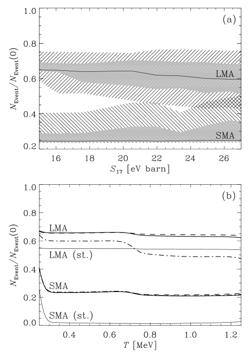
FIG. 6.: (a) Event rates in Borexino normalized to the expected rates from our standard solar model without oscillations for different values of $S_{\rm 17}$. The shaded regions show the 1$\sigma$, the hatched the 2$\sigma$ areas. (b) Recoil electron spectrum for the best fit SMA and LMA solutions in sterile (st.) and non-sterile case. For the latter $S_{\rm 17}=15$ (dashed), 19 (solid) and 27 (dash-dotted) in units of ${\rm eV\,barn}$.

behaviour of the SMA solution is described by the typical shape of the survival probability of electron neutrinos with varying energy (“valley” at intermediate energies). This leads to an almost full conversion of the ${}^{7}\rm{Be}$-neutrinos into $\nu_{\tau},\nu_{\mu}$ or $\nu_{\rm s}$, partial conversion of the ${\rm{}^{8}B}$-neutrino and almost no change of the $pp$-neutrinos. In the case of the LMA-solution the survival probability of $\nu_{\rm e}$ is almost constant for all the energies. In the light of the present solar neutrino experiments results (total rates) the MSW-SMA solution seems to be the most viable one for explaining the lack of ${}^{7}{\rm Be}$ and a reduction by a factor 2 of the ${}^{8}{\rm B}$ neutrinos.

In the VO case ($10^{-11}$$\leq$$\Delta m^{2}$$\leq$$10^{-9}$) the eccentric orbit of the earth leads to seasonal variations in the neutrino flux due to the long oscillation length $l_{\rm V}\approx 2.48E/\Delta m^{2}$ ($l_{\rm V}$ in m, $E$ in MeV, $\Delta m^{2}$ in $eV^{2}$). Since 90% of the ${}^{7}{\rm Be}$-neutrinos are emitted in a monoenergetic line, this effect is more pronounced for these neutrinos than for $pp$ and ${}^{8}{\rm B}$-neutrinos, which are emitted in a continuous range of energies. In the SMA and LMA solutions no seasonal variation appears, thus Borexino should be able to discriminate between these cases and the VO solution (i).

C SNO

The SNO experiment will measures the recoil electron spectrum of the reaction

$\displaystyle\nu_{e}+d\rightarrow p+p+e^{-}$

and the ratio of the charged to neutral current events (CC/NC). Using the neutrino fluxes of a solar model with a fixed value of $S_{17}$, the expected (CC/NC)-ratio is determined by letting $\Delta m^{2}$ and $\sin^{2}2\theta$ vary within the 68.4% and 95.4% C.L.-region of the LMA, SMA or VAC-solution. As shown in Fig. 3, varying $S_{17}$ change the oscillation parameters which are able to reproduce the present results of GALLEX/SAGE, SK and HM. These changes alter the expected (CC/NC)-ratio, and thus provide an indirect dependence of the (CC/NC)-ratio on $S_{17}$ (ii). The found relations are shown in Fig. 7. For the calulation of the (CC/NC)-ratio in SNO we have used the energy resolution corresponding to a typical statistics of 5000 CC events.

FIG. 7.: (CC/NC)-ratio in SNO for solar models with varying values of $S_{\rm 17}$. The dashed line shows the $1\sigma$, the dash-dotted line the $2\sigma$-range.

In the case of VO solution the $1\sigma$ level of uncertainty is significantly larger than in the MSW solution case (Fig. 7). In the SMA scenario it is possible to determine an effective constraint on $S_{17}$ from the $1\sigma$-level strip of the (CC/NC) ratio. For instance, from Fig. 7 it can be inferred that a measurement of (CC/NC) of $\simeq 0.8$ would imply

$\displaystyle S_{17}=19.0^{+2.0}_{-3.0}~{}{\rm keV\,barn},$

if SMA turns out to be the solution of the solar neutrino puzzle. In the VO case the limits are not very stringent but they nevertheless provide independent constraints on the allowed value of $S_{17}$. However, this procedure is not very useful for sterile neutrinos, because no sensible variation of the (CC/NC) ratio occurs when $S_{17}$ is varied.

The recoil electron spectrum provides additional information about the type of the solution (i). In particular we have employed a Gaussian energy resolution function of width $\sigma_{10}=1~{}{\rm MeV}$ at the electron energy $E_{\rm e}=10~{}{\rm MeV}$ as adopted in  [26]. For the best fit SMA and LMA solutions obtained from solar models with different values of $S_{17}$, the expected electron energy spectrum in SNO is shown in Fig. 8 for the case of active neutrinos.

FIG. 8.: Normalized electron energy spectra in SNO for active neutrinos. The SMA solutions correspond to the solid and dashed lines for $S_{17}=14~{}{\rm eV\,barn}$ and $S_{17}=23~{}{\rm eV\,barn}$ respectively. The dash-double-dotted ($S_{17}=23~{}{\rm eV\,barn}$) and dash-dotted lines ($S_{17}=14~{}{\rm eV\,barn}$) are for the LMA solution.

The separation in the recoil electron spectra of both solutions is not very pronounced, therefore these data alone may not be sufficient to discriminate between LMA and SMA solution. We remark that the overall behaviour of the SMA and LMA solutions in SNO is very similar to the one in SK, namely that the average energy of the recoil electrons is higher in the SMA than in the LMA case for every value of $S_{17}$ (see also Table IV).

In the sterile case the differences among various cases with altered $S_{17}$ are much smaller (ii), and it is even more unlikely that any significant variation in the spectra will be visible, neither in SNO nor in SK.

V Conclusions

We have investigated the influence of $S_{11}$ on the sound speed and the small spacing frequency differences by comparing the model predictions with helioseismic data using up-to-date solar models. Moreover we discussed the change in the allowed parameter space for SMA, LMA and VO solutions with varying $S_{17}$. As shown in Section II the latest results from helioseismology suggest that the value of $S_{11}$ is slightly greater than the theoretically calculated one. However, since the statistical significance is weak, we conclude that the limits inferred from helioseismology and those derived from the theory are consistent. The influence of the value of $S_{11}$ on the solar neutrino flux is too small to alter the resulting neutrino mixing parameters significantly. However, the proposed LENS detector [27] can observe in principle a suppression of the $pp$-neutrino flux and therefore it is reasonable to expect relevant differences in the signal as function of the $S_{11}$ value.

The present experiments GALLEX/SAGE, HM and SK favour neutrino oscillations as the solution to the solar neutrino deficit. Improved statistics in SK and future experiments like Borexino and SNO will provide powerful tools to support this solution. We have calculated the expected rates, electron moments, electron spectra or (CC/NC)-ratios of the above experiments for the SMA, LMA and VO solution provided by the present data. We expect that the combined data of the recoil electron spectra in SK, SNO and Borexino enable us to discriminate among these solutions.

Since the ${}^{7}{\rm Be}(p,\gamma)^{8}{\rm B}$ reaction has no influence on the solar structure, it is impossible to get information about its strength from helioseismology. Moreover the exact value for $S_{17}$ is crucial to calculate the flux of the most energetic solar neutrinos, which are measured in the SK and SNO experiments. The (CC/NC)-ratio expected in SNO is sensitive to the $\phi_{\nu}(^{8}{\rm B})$ which is directly related to the strength of $S_{17}$.

We conclude that the combination of SK, SNO and Borexino will be useful to test the consistency of the value of $S_{17}$ found by direct nuclear physics measurements with the combined analysis of theoretical models and neutrino experiments as described in Sections III and IV. Of course, the whole analysis was done under the assumption of neutrino-oscillations (either MSW or “just so”) as solution to the solar neutrino puzzle. In the case of oscillations into sterile neutrinos the strength of ${}^{7}{\rm Be}({\rm p},\gamma)^{8}{\rm B}$ does not leave any signature in the future experiments. However, this solution can be at least discriminated from the oscillations into active neutrinos by means of the behaviour of the (CC/NC) ratio.

REFERENCES

- [1] S. P. Mikheyev and A. Y. Smirnov, Sov. J. Nucl. Phys. 42, 913 (1985); L. Wolfenstein, Phys. Rev. D 17, 2369, (1978).
- [2] B. Pontecorvo, Sov. Phys. JETP 26, 984 (1968); J. N. Bahcall and S. C. Frautschi, Phys. Lett. 29B, 623 (1969); S. M. Bilenky and B. M. Pontecorvo, Phys. Rep. 41, 225 (1978).
- [3] J. N. Bahcall, M. H. Pinsonneault and G. J. Wasserburg, Rev. Mod. Phys. 67, 885, (1995).
- [4] P. D. Parker and C. Rolfs, in Solar Interior and Atmosphere, edited by A. N. Cox, W. C. Livingston, and M. S. Matthews (The University of Arizona Press, 1991), p. 31.
- [5] M. Kamionkowski and J. N. Bahcall, Astrophys. J. 420, 884 (1994).
- [6] E. G. Adelberger et al., Rev. Mod. Phys. 70, 1265 (1998).
- [7] S. Turck-Chièze et al., Phys. Rep. 230, 57 (1993).
- [8] L. Paternò, in Fouth International Neutrino Confernce, edited by W. Hampel (Max-Planck-Institut für Kernphysik, Heidelberg, 1997), p. 54.
- [9] J. N. Bahcall and A. Ulmer, Phys. Rev. D 53 4202, (1996);
- [10] N. Hata and P. Langaker, Phys. Rev. D 52, 420, (1995); P. Krastev and A. Smirnov, Phys. Lett. B338, 282 (1994); P. I. Krastev and S. T. Petcov, Phys. Lett. B395, 69, (1997).
- [11] R. Kippenhahn, A. Weigert, and E. Hofmeister, in Methods for Calculating Stellar Evolution, Vol. 7 of Methods in Computational Physics (New York: Academic Press, 1967), p. 129.
- [12] H. Schlattl, A. Weiss, and H.-G. Ludwig, Astron. Astrophys. 322, 64 (1997).
- [13] C. A. Iglesias and F. J. Rogers, Astrophys. J. 464, 943 (1996).
- [14] F. J. Rogers, F. J. Swenson, and C. A. Iglesias, Astrophys. J. 456, 902 (1996).
- [15] A. A. Thoul, J. N. Bahcall, and A. Loeb, Astrophys. J. 421, 828 (1994).
- [16] N. Grevesse and A. Noels, Phys. Scripta T47, 133 (1993).
- [17] E. Vitense, Z. Astrophys. 32, 135 (1953).
- [18] H. Schlattl and A. Weiss, submitted to Astron. Astrophys. (1999).
- [19] S. Turck-Chièze et al., Sensitivity of the Sound Speed to the Physical Processes Included in the Standard Solar Model, 1998, ed. by S. Korzennik and A. Wilson, ESA-SP 418, 555, (ESA Publication Division, Noordwijk , Netherlands).
- [20] M. Lazrek et al., Sol. Phys. 175, 227 (1997).
- [21] H. M. Antia and S. M. Chitre, Astron. Astrophys. 339, 239 (1998).
- [22] J. N. Bahcall, S. Basu, and M. H. Pinsonneault, Phys. Lett. B 433, 1 (1998).
- [23] J. Bouchez et al., Z. Phys. C 32, 499 (1986). M. Cribier, W. Hampel, J. Rich and D. Vignaud, Phys. Lett. B 182, 89 (1986). A. J. Baltz and J. Wesener, Phys. Rev. D 35, 528 (1987); ibid. 37, 3364 (1988). A. Dar, A. Mann, Y. Melina and D. Zajfman, Phys. Rev. D 35, 3607 (1987). A. Dar and A. Mann, Nature (London) 325, 790 (1987). S. P. Mikeyev and A. Yu. Smirnov, in Moriond ’87, Proceedings of the 7th Moriond Workshop on New and Exotic Phenomena, Les Arcs, 1987, edited by O. Fackler and J. Trân Thanh Vân (Frontières, Paris, 1987), p. 405. M. L. Cherry and K. Lande, Phys. Rev. D 36, 3571 (1987). S. Hiroi, H. Sakuma, T. Yanagida and M. Yoshimura, Phys. Lett. B 198, 403 (1987); Prog. Theor. Phys. 78, 1428 (1987). M. Spiro and D. Vignaud, Phys. Lett. B 242, 279 (1990).
- [24] The Super-Kamiokande Collaboration, Y. Fukuda et al., hep-ex/9812009 (1998).
- [25] The Super-Kamiokande Collaboration, Y. Fukuda et al., hep-ex/9812011 (1998).
- [26] J. N. Bahcall, P. I. Krastev and E. Lisi, Phys. Rev. C 55, 494, (1997).
- [27] R. S. Raghavan, Phys. Rev. Lett. 19, 3618, (1997).