Measuring and Modelling the Redshift Evolution of Clustering: the Hubble Deep Field North

Abstract

The evolution of galaxy clustering from $z=0$ to $z\simeq 4.5$ is analyzed using the angular correlation function and the photometric redshift distribution of galaxies brighter than $I_{AB}\leq 28.5$ in the Hubble Deep Field North. The reliability of the photometric redshift estimates is discussed on the basis of the available spectroscopic redshifts, comparing different codes and investigating the effects of photometric errors. The redshift bins in which the clustering properties are measured are then optimized to take into account the uncertainties of the photometric redshifts. The results show that the comoving correlation length $r_{0}$ has a small decrease in the range $0\raise-2.0pt\hbox{\hbox to0.0pt{\hbox{$\sim$}\hss}\raise 5.0pt\hbox{$<$}\ }z\raise-2.0pt\hbox{\hbox to0.0pt{\hbox{$\sim$}\hss}\raise 5.0pt\hbox{$<$}\ }1$ followed by an increase at higher $z$. We compare these results with the theoretical predictions of a variety of cosmological models belonging to the general class of Cold Dark Matter scenarios, including Einstein-de Sitter models, an open model and a flat model with non-zero cosmological constant. The comparison with the expected mass clustering evolution indicates that the observed high-redshift galaxies are biased tracers of the dark matter with an effective bias $b$ strongly increasing with redshift. Assuming an Einstein-de Sitter universe, we obtain $b\simeq 2.5$ at $z\simeq 2$ and $b\simeq 5$ at $z\simeq 4$. These results support theoretical scenarios of biased galaxy formation in which the galaxies observed at high redshift are preferentially located in more massive halos. Moreover, they suggest that the usual parameterization of the clustering evolution as $\xi(r,z)=\xi(r,0)\ (1+z)^{-(3+\epsilon)}$ is not a good description for any value of $\epsilon$. A comparison of the clustering amplitudes that we measured at $z\simeq 3$ with those reported by Adelberger et al. (1998) and Giavalisco et al. (1998), based on a different selection, suggests that the clustering depends on the abundance of the objects: more abundant objects are less clustered, as expected in the paradigm of hierarchical galaxy formation. The strong clustering and high bias measured at $z\simeq 3$ are consistent with the expected density of massive haloes predicted in the frame of the various cosmologies considered here. At $z\simeq 4$, the strong clustering observed in the Hubble Deep Field requires a significant fraction of massive haloes to be already formed by that epoch. This feature could be a discriminant test for the cosmological parameters if confirmed by future observations.

1 Introduction

Clustering properties represent a fundamental clue about the formation and evolution of galaxies. Several large spectroscopic surveys have measured the correlation function of galaxies in the local universe, studying its dependence on morphological type or absolute magnitude (Santiago & da Costa 1990; Park et al. 1994; Loveday et al. 1995; Benoist et al. 1996; Tucker et al. 1997). Higher values of the correlation length $r_{0}$ are observed for elliptical galaxies (or galaxies with brighter absolute magnitude), while lower values are obtained for late type galaxies (or galaxies with fainter absolute magnitude). This difference in the clustering strength suggests that the various galaxy populations are not related in a straightforward way to the distribution of the matter. To account for these observations, one has to consider as a first approach that galaxies are biased tracers of the matter distribution as $\xi_{\rm gal}(r)=b^{2}({\cal M})\xi_{\rm m}(r)$ (Kaiser 1984), where $\xi_{\rm gal}(r)$ refers to the spatial correlation function of the galaxies, $\xi_{\rm m}(r)$ refers to the spatial correlation function of the mass and $b({\cal M})$ represents the bias associated with different galaxy populations. Here ${\cal M}$ describes the intrinsic properties of the objects (like mass, luminosity, etc).

Deep spectroscopic surveys have made it possible to reach higher redshifts and study the evolution of galaxy clustering. For example the Canada-France Redshift Survey (CFRS; Le Fèvre et al. 1996) samples the universe up to $z\simeq 1$ while the K-selected galaxy catalogue by Carlberg et al. (1997) reaches $z\simeq 1.5$. From these data it has been possible to find a clear signal for evolution in the clustering strength: the correlation length is three times smaller at high redshifts ($z\simeq 1$) than its local value. In addition, Carlberg et al. (1997) have found segregation effects between the red and blue samples similar to those observed locally. A common approach is to assume that the galaxy sample traces the underlying mass density fluctuation [$b({\cal M},z)=1$, or at least $b({\cal M},z)=constant$], and fit the clustering evolution of the mass with a parametric form: $\xi(r,z)=\xi(r,0)(1+z)^{-(3+\epsilon)}$ (Peebles 1980), where $\epsilon$ describes the evolution of the mass distribution due to the gravitational instability. Such an assumption makes it straightforward to discriminate between different cosmological models. From N-body simulations, Colín, Carlberg & Couchman (1997) found faster evolution in the Einstein-de Sitter (hereafter EdS) universe than in an open universe with matter density parameter $\Omega_{\rm 0m}=0.2$ ($\epsilon\simeq 0.8$ and $\epsilon=0.2$, respectively). Carlberg et al. (1997) obtained from their data a small value of $\epsilon$ which would be quite difficult to reconcile with an EdS universe, while Le Fèvre et al. (1996) found a value $0\leq\epsilon\leq 2$, still consistent with any fashionable cosmological model. However, using directly the galaxy clustering evolution to derive the relevant properties of the mass is a questionable practice, due to the bias acting as a complicating factor. Different samples select a mixture of galaxy masses and the effective bias, which is expected in current hierarchical galaxy formation theories to depend on redshift and mass [i.e. $b({\cal M},z)$], plays a key role in the observed evolution of clustering. Exciting progress in this field has been achieved with the recent discovery of a large number of galaxies at $z\simeq 3$ (Lyman-Break Galaxies, hereafter LBGs) using the U-dropout technique (Steidel et al. 1996). For the first time, the high-$z$ universe is probed via a population of quite “normal” galaxies in contrast with the previous surveys dominated by QSOs or radio galaxies. The LBG samples offer the opportunity to estimate in a narrow time-scale ($2.6\leq z\leq 3.4$) number densities, luminosities, colours, sizes, morphologies, star formation rates (SFR), chemical abundances, dynamics and clustering of these primordial galaxies. By using different catalogues and statistical techniques, Giavalisco et al. (1998, hereafter G98) and Adelberger et al. (1998, hereafter A98) have measured the correlation length $r_{0}$ of this population. The values they found are at least comparable to that of present-day spiral galaxies ($r_{0}=2-4\ h^{-1}$ Mpc when an EdS universe is assumed). Such a strong clustering at $z\simeq 3$ is inconsistent with clustering evolution modeled in terms of the $\epsilon$ parameter for any value of $\epsilon$ (G98). By comparing the correlation amplitudes with the predictions for the mass correlation, G98 and A98 obtained (for an EdS universe) a linear bias $b\simeq 4.5$ and $b\simeq 6$, respectively. These results suggest that the LBGs formed preferentially in massive dark matter haloes.

An alternative way to extend the present information over a larger range of redshifts is to use the photometric measurements of redshifts in deep multicolor surveys. This technique, based on the comparison between theoretical (and/or observed) spectra and the observed colours in various bands, makes it possible to derive a redshift estimate for galaxies which are one or two magnitudes fainter than the deepest limit for spectroscopic surveys (even with 10 m-class telescopes).

An optimal combination of deep observations and the photometric redshift technique has been attained with the Hubble Deep Field (HDF) North. Photometric redshifts have been used to search for high-redshift galaxies (Lanzetta, Yahil & Fernández-Soto 1996) and investigate the evolution of their luminosity function and SFR (Sawicki, Lin & Yee 1996; Madau et al. 1996; Gwyn & Hartwick 1996; Franceschini et al. 1998), their morphology (Abraham et al. 1996; van den Bergh et al. 1996; Fasano et al. 1998) and clustering properties (Connolly, Szalay & Brunner 1998; Miralles & Pelló 1998; Magliocchetti & Maddox 1999; Roukema et al. 1999). A critical issue is the statistical uncertainty of the photometric redshifts which strongly depends on the number of bands following at the various redshifts the main features of a galaxy spectral energy distribution (hereafter SED), in particular the 4000 Å break and the 912 Å Lyman break.

The aim of this paper is to measure the galaxy clustering evolution in the full redshift range $0\leq z\leq 4.5$, using the photometric redshifts of a galaxy sample with $I_{AB}\leq 28.5$ in the HDF North (including infrared data, i.e. Fernández-Soto, Lanzetta & Yahil 1999, hereafter FLY99) and carry out an extended comparison of the results with the theoretical predictions of different current galaxy formation scenarios based on variants of the Cold Dark Matter model. This comparison will be performed using the techniques introduced by Matarrese et al. (1997) and Moscardini et al. (1998), which allow a detailed modelling of the evolution of galaxy clustering, accounting both for the non-linear dynamics of the dark matter distribution and for the redshift evolution of the galaxy-to-mass bias factor.

Our sample probes a population fainter than the spectroscopic LBGs and an inter-comparison of their clustering properties will be useful to address the differences in the nature of the two populations. However, the photometric redshift approach should be used with some caution when reaching such faint limits. In fact, uncertainties and systematic errors are expected to be larger than those estimated in the comparison of photometric and spectroscopic redshifts, which is typically limited to $I_{AB}\leq 26$. This problem is particularly relevant for the analysis of the angular correlation function since in this statistic all galaxies at a given redshift contribute with the same weight. This is different, for example, to what happens when these objects are used to estimate the star formation rate history, where brighter objects, with smaller uncertainties in the redshift determination, have more weight. For these reasons we try to provide a rough estimate of the errors in the redshift estimates at faint magnitudes, by comparing the results of different photometric redshift techniques and by using Monte Carlo simulations. This in turn provides the necessary information to define optimal redshift bin sizes (i.e. minimizing the effects of the redshift uncertainties) for the clustering analysis.

The plan of the paper is as follows. In Section 2, we present the photometric database and we describe the photometric redshift technique. In Section 3, we investigate the reliability of the photometric redshift estimates. In Section 4, we present the results for the angular correlation function computed in different redshift ranges. Section 5 is devoted to a comparison of these results with the theoretical predictions of different cosmological models belonging to the general class of the Cold Dark Matter scenario. Finally, discussion and conclusions are presented in Section 6.

2 The photometric redshift measurement

2.1 The photometric database

As a basis for the present work, we have used the photometric catalogue produced by FLY99 on the HDF-North using the source extraction code SExtractor (Bertin & Arnouts 1996). In addition to the four optical WFPC2 bands (Williams et al. 1996), infrared observations in J, H and Ks bands (Dickinson et al. 1999) are incorporated.

A particularly valuable feature of the FLY99 catalogue is that the optical images are used to model spatial profiles that are fitted to the infrared images in order to measure optimal infrared fluxes and uncertainties. In this way, for the large majority of the objects, an estimate of the infrared flux is available down to the fainter magnitudes. This is a definite advantage for the derivation of photometric redshifts.

The analysis described below has been applied to the F300W, F450W, F606W, F814W, J, H, Ks magnitudes of 1023 objects down to $I_{AB}\simeq 28.5$ (here we note that the magnitude $I_{AB}$ refers directly to the photometric catalogue given by FLY99 and not to their best fit $I_{AB}$ reported in their photometric redshift catalogue).

2.2 The photometric redshift technique

Various authors have explored a number of different approaches to estimate redshifts of galaxies from deep broad-band photometric databases. Empirical relations between magnitudes and/or colours and redshifts have been calibrated using spectroscopic samples (Connolly et al. 1995; Wang, Bahcall & Turner 1998). Other techniques are based on the comparison of the observed colours of galaxies with those expected from template SEDs, either observed (Lanzetta et al. 1996; FLY99) or theoretical (Giallongo et al. 1998) or a combination of the two (Sawicki, Lin & Yee 1997; hereafter SLY97). Bayesian estimation has also been used (Benítez 1998).

2.2.1 The synthetic spectral libraries

The type of approach followed in the present work is based on the comparison of observed colours with theoretical SEDs and has been described by Giallongo et al. (1998). Here we summarize its main ingredients:

1. The SEDs are derived from the GISSEL library (Bruzual & Charlot 1999). The spectral synthesis models are governed by a number of free parameters listed in Table 1. The star formation rate for a galaxy with a given age is governed by the assumed e-folding star formation time-scale $\tau$. Several values of $\tau$ and galaxy ages are necessary to reproduce the different observed spectral types. We also have to assume a shape for the initial mass function (IMF). As shown by Giallongo et al. (1998), the photometric redshift estimate is not significantly changed by using different IMFs. Here we restricted our analysis to a Salpeter IMF.

2. In addition to the GISSEL parameters, we have added the internal reddening for each galaxy by applying the observed attenuation law of local starburst galaxies derived by Calzetti, Kinney & Storchi-Bregmann (1994) and Calzetti (1997). The different values of the reddening excess are listed in Table 1. We have also included the Lyman absorption produced by the intergalactic medium as a function of redshift in the range $0\leq z\leq 5$, following Madau (1995).

As a result we obtained a library of $2.5\times 10^{5}$ spectra, which can be used to derive the colours as a function of redshift for all the model galaxies with an age smaller than the Hubble time at the given redshift (which is cosmology-dependent; the adopted cosmological parameters are also given in Table 1).

Table 1: Parameters used for the library of templates

IMF	Salpeter
Exponential SFR
Timescales $\tau$ (Gyr)	1,2,3,5,9,$\infty$,2 bursts
Ages (Gyr)	.01,.05,.1,.25,.5,.75,1.,1.5,2.,
	3.,4.,5.,6.,7.,8.,9.,10.,11.,12.,14.
Metallicities	$Z_{\odot}$, 0.2$Z_{\odot}$, 0.02$Z_{\odot}$
$E_{B-V}$	0,0.05,0.1,0.2,0.3,0.4
Extinction Law	Calzetti
Cosmology ($H_{0}$, $q_{0}$)	50, 0.5

2.2.2 Estimating redshifts

To measure the photometric redshifts we used a standard $\chi^{2}$ fitting procedure comparing the observed fluxes $F_{\rm obs}$ (and corresponding uncertainties) with the GISSEL templates $F_{\rm tem}$:

$$\chi^{2}=\sum_{i}\left[{F_{{\rm obs},i}-s\cdot F_{{\rm tem},i}\over\sigma_{i}}\right]^{2}\ ,$$ (1)

where $F_{{\rm obs},i}$ and $\sigma_{i}$ are the fluxes observed in a given filter $i$ and their uncertainties, respectively; $F_{{\rm tem},i}$ are the fluxes of the template in the same filter; the sum runs over the seven filters. The template fluxes have been normalized to the observed ones by choosing the factor $s$ which minimizes the $\chi^{2}$ value ($\partial\chi^{2}/\partial s=0$):

$$s=\sum_{i}\left[{F_{{\rm obs},i}\cdot F_{{\rm tem},i}\over\sigma_{i}^{2}}\right]\Big{/}\sum_{i}\left[{F_{{\rm tem},i}^{2}\over\sigma_{i}^{2}}\right]\ .$$ (2)

In the GISSEL library the models provide fluxes emitted per unit mass (in $M_{\odot}$) and the normalization parameter $s$, which rescales the template fluxes to the observed ones, provides a rough estimation of the observed galaxy mass. We have limited the range of models accepted in the $\chi^{2}$ comparison to the interval $10^{7}$–$10^{14}\ M_{\odot}$. We derived the $\chi^{2}$ probability function (CPF) as a function of $z$ using the lowest $\chi^{2}$ values at any redshift. To have an idea of the redshift uncertainties we have derived the interval corresponding to the standard increment $\Delta\chi^{2}=1$. At the same time the CPF is analyzed to detect the presence, if any, of secondary peaks with a multi-thresholding algorithm (typically we decompose the normalized CPF into ten levels).
We notice that our estimates of the photometric redshifts are changed by less than 2% if we adopt a different cosmology [($\Omega_{\rm 0m}=0.3$, $\Omega_{\rm 0\Lambda}=0$) or ($\Omega_{\rm 0m}=0.3$, $\Omega_{\rm 0\Lambda}=0.7$)] and our mass estimates are nearly unchanged.

3 Comparison with previous works and simulations

3.1 Spectroscopic vs. photometric redshifts

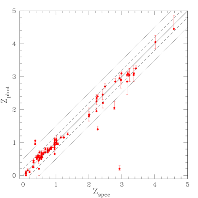
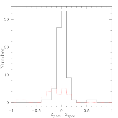
In Figure 1 we show the comparison of our estimates of the photometric redshifts $z_{\rm phot}$ with the 106 spectroscopic redshifts $z_{\rm spec}$ up to $z\simeq 5$ listed in the FLY99 catalogue (see references therein). Our values are generally consistent with the observed spectroscopic redshifts within the estimated uncertainties over the full redshift range. The r.m.s. dispersion $\sigma_{z}$ for different redshift intervals is reported in Table 2. At redshifts lower than 1.5, two galaxies have photometric redshifts which appear clearly discrepant: galaxy # 191 (the number refers to the FLY99 number) with $z_{\rm phot}\simeq 1.05$ vs. $z_{\rm spec}\simeq 0.37$ and galaxy # 619 with $z_{\rm phot}\simeq 0.95$ vs. $z_{\rm spec}\simeq 0.37$. Also FLY99 and SLY97 found for these two objects $z_{\rm phot}\geq 0.88$. As discussed in the next section, the techniques used in SLY97, in FLY99 and in the present work are significantly different; therefore, if the spectroscopic redshifts are correct, both objects are expected to have a really peculiar SED. For example, various SEDs used in these works do not include spectra with strong emission lines (starbursts, AGN, …). Yet, based on the observed spectra, the two spectroscopic redshifts are very uncertain (see http://astro.berkeley.edu/davisgrp/HDF/). Disregarding these two objects, the photometric accuracy at $z<1.5$ decreases from $\sigma_{z}\simeq 0.13$ to $\sigma_{z}\simeq 0.09$. These values are consistent with the photometric redshift estimates obtained in previous works and compiled by Hogg et al. (1998).

At redshifts $z\geq 1.5$ the dispersion is $\sigma_{z}=0.24$, if the galaxy # 687, which shows catastrophic disagreement (it is found at low redshift also by FLY99, while there is no clear association in the SLY97 catalogue) is discarded. Direct inspection of the original frames shows that in this case the photometry can be incorrect due to the complex morphology of this object, which was assumed to be a single unit.

Figure 1: The left panel shows the comparison of our photometric redshifts $z_{\rm phot}$ with the spectroscopic ones $z_{\rm spec}$. Error bars represent the region where $\Delta\chi^{2}\leq 1$. The dotted and long-dashed lines represent $\Delta z=0.5$ and $\Delta z=0.2$, respectively. The right panel shows the histograms with $z_{\rm phot}-z_{\rm spec}$ for galaxies with $z_{\rm spec}\leq 1.5$ (solid line) and $z_{\rm spec}>1.5$ (dotted line).

Table 2: Comparison of our photometric redshifts with 106 spectroscopic redshifts up to $z=5$ for different redshift intervals (Column 1). Here we consider only objects either with $|\Delta z|\equiv|z_{\rm spec}-z_{\rm phot}|\leq 1$ or with $|\Delta z|\leq 0.5$ (Column 2). The corresponding number of objects in each redshift interval is given in Column 3 and the associated dispersion $\sigma_{z}$ in Column 4.

$z$ range	$|\Delta z|$	$N_{\rm phot}$/$N_{\rm spec}$	$\sigma_{z}$
0.0 - 5.0	$\leq$ 1.0	105/106	0.20
0.0 - 1.5	$\leq$ 1.0	79/79	0.13
1.5 - 5.0	$\leq$ 1.0	28/29	0.24
0.0 - 5.0	$\leq$ 0.5	101/106	0.12
0.0 - 1.5	$\leq$ 0.5	77/79	0.09
1.5 - 5.0	$\leq$ 0.5	26/29	0.15

3.2 Comparison with other photometric redshifts

The relatively good agreement of the photometric redshifts with the spectroscopic ones shows the reliability of our method at bright magnitudes. Obviously, the same accuracy cannot be expected also at fainter magnitudes, below the spectroscopic limit $I_{AB}\geq 26$. The uncertainty in the identification of the characteristic features (4000 Å and Lyman break) in the observed SEDs necessarily increases when the errors in the photometry become larger. In order to obtain a rough idea of the uncertainty also in the domain inaccessible to spectroscopy we have compared the results of our code with those obtained with other photometric methods.

FLY99 and SLY97 have used the four spectra provided by Coleman, Wu & Weedman (1980) which reproduce different star formation histories or different galaxy types (E/S0, Sbc, Scd and Irr). The wavelength coverage of these template spectra is however too small (1400 - 10000 Å) to allow a direct comparison with the full range of photometric data (3000 - 25000 Å). To bypass this problem, both authors have extrapolated the infrared SEDs by using the theoretical SEDs of the GISSEL library, corresponding to the four spectral types. In the UV SLY97 have used again an extrapolation based on GISSEL while FLY99 have used the observations of Kinney et al. (1993). SLY97 have enlarged the SED library with two spectra of young galaxies with a constant star formation (from the GISSEL library) and interpolated between the six spectra to reduce the aliasing effect due to the SED sparse sampling.

The comparison of the two approaches with spectroscopic redshifts has been carried out by the authors: the uncertainties are typically $\sigma_{z}\simeq 0.10-0.15$ at $z\leq 1.5$ and reach $\sigma_{z}\simeq 0.20-0.25$ at higher redshifts.

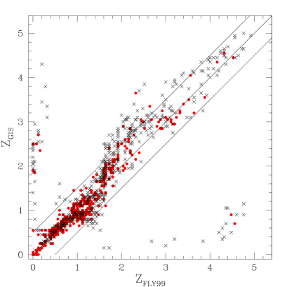
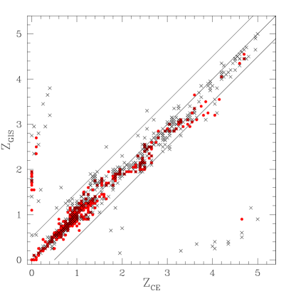
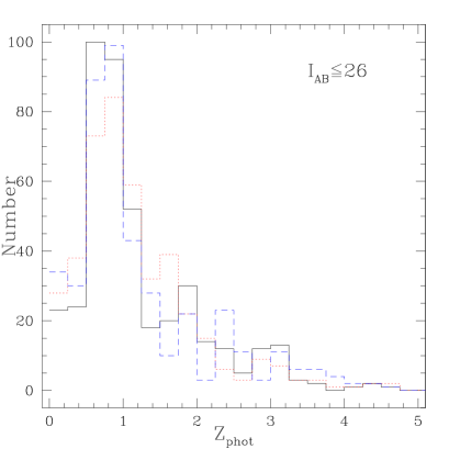
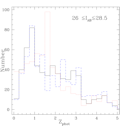
In the SLY97 analysis, only the four optical bands have been used to estimate the photometric redshifts. To carry out a fair comparison, we have set up a code based on a library similar to that used by SLY97 and we recomputed the photometric redshifts with the FLY99 catalogue (hereafter called Coleman Extended model: CE). The comparison between the three methods is shown in Figure 2 (upper panels). The three redshift distributions are shown in the lower panels of the the same figure. From these plots, we observe that:

1. For $I_{AB}\leq 26$ the three methods are compatible within $\Delta z\simeq 0.5$. A small number ($\sim$ 2%) of catastrophic discrepancies ($\Delta z\geq 1$) is observed. Excluding these objects, we find r.m.s. dispersions $\sigma_{z}\simeq 0.12$ and $\sigma_{z}\simeq 0.23$ between the GISSEL and CE models at $z\leq 1.5$ and $1.5<z\leq 5$, respectively. In the high-redshift range a systematic shift is observed with $\langle z_{\rm GIS}-z_{\rm CE}\rangle\simeq-0.15$. Between the GISSEL and FLY99 models, the dispersions are $\sigma_{z}\simeq 0.16$ and $\sigma_{z}\simeq 0.26$ at $z\leq 1.5$ and $1.5<z\leq 5$, respectively, with a systematic shift in the high-redshift range $\langle z_{\rm GIS}-z_{\rm FLY99}\rangle\simeq+0.18$. These results are compatible with the uncertainties based on the spectroscopic sample. Finally the three resulting redshift distributions are in good agreement.

2. For $I_{AB}\leq 28.5$ the number of objects with $\Delta z\geq 1$ increases and represents the 6% of the full sample in both cases. Excluding these objects, we find dispersions $\sigma_{z}\simeq 0.18$ and $\sigma_{z}\simeq 0.26$ between the GISSEL and CE models at $z\leq 1.5$ and $1.5<z\leq 5$, respectively. For the high-redshift range a systematic shift is still observed with $\langle z_{\rm GIS}-z_{\rm CE}\rangle\simeq-0.11$. Comparing the GISSEL and FLY99 models, the dispersions are $\sigma_{z}\simeq 0.22$ and $\sigma_{z}\simeq 0.32$ at $z\leq 1.5$ and $1.5<z\leq 5$, respectively, with a larger systematic shift in the high-redshift range $\langle z_{\rm GIS}-z_{\rm FLY99}\rangle\simeq+0.31$.

3. The large shift for $z\geq 1.5$ observed with FLY99 is due to a feature appearing in their redshift distribution with a large number of sources between $1.2\leq z\leq 2$, not observed in the two other models (Figure 2, lower right panel). The interval $1.2\leq z\leq 2$ is critical for the photometric determination of the redshifts, due to the lack of strong features. In fact the Lyman-alpha break is not yet observed in the $F300W$ band and the break at $4000$ Å is located between the $F814W$ and $J$ bands. Therefore the estimates rest basically on the continuum shape of the templates. As shown by FLY99 in their Figure 6, their photometric redshifts suffer from a systematic underestimate with respect to the spectroscopic ones around $z\simeq 2$. This may be due to an inadequacy of the UV extrapolation used by FLY99 in reproducing the UV shape of the high-$z$ objects. This effect disappears at higher redshifts because of the U-dropout effect. As a check, we have added to the four templates of FLY99 a spectrum of an irregular galaxy with constant star formation rate (with higher UV flux). In this case the excess of galaxies with $1.2\leq z\leq 2$ disappears and the objects are re-distributed in better agreement with the two other methods.

4. Our GISSEL model produces a smaller number of objects at $z\geq 3.5$ with respect to the two other approaches. The discrepant objects (found at lower redshift by the GISSEL code) are generally fitted by using a significant fraction of reddening excess ($\langle{\rm E(B-V)}\rangle\simeq 0.3$). Note that in general objects found at $z\geq 3.5$ by the GISSEL code are also at high redshift with the other techniques.

Figure 2: Comparison of our photometric redshifts $z_{\rm GIS}$ (computed using the GISSEL library) with the photometric redshifts obtained by FLY99 ($z_{\rm FLY99}$; upper left panel) and with our Coleman Extended (CE) libraries similar to the SLY97 method ($z_{\rm CE}$; upper right panel). Filled circles represent objects with $I_{AB}\leq 26$ and crosses refer to objects with $26\leq I_{AB}\leq 28.5$. Solid lines correspond to $\Delta z=0.5$. In the two lower panels, we show the comparison of the three redshift histograms for $I_{AB}\leq 26$ (left panel) and $26<I_{AB}\leq 28.5$ (right panel). Our GISSEL model, the CE model and the FLY99 model are shown by solid, dashed and dotted lines, respectively.

3.3 Comparison with the NICMOS F110W and F160W observations

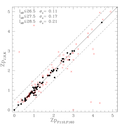
Recently, deep NICMOS images have been obtained in the area corresponding to chip 4 of the WFPC2 camera in the HDF-North (Thompson et al. 1999). The observations have been carried out in the two filters $F110W$ and $F160W$ and reach $F160W_{AB}\simeq 28.8$ (at 3$\sigma$). We have associated each NICMOS detection (from the published catalogue) with the FLY99 catalogue. We consider in our analysis the 164 objects detected in both NICMOS filters. These data provide a crucial check thanks to their depth and high spatial resolution and also to the spectral coverage of the $F110W$ band. This filter fills the gap between the $F814W$ filter and the standard $J$ filter and makes it possible to detect the 4000 Å break at $z\geq 1.2$. We have recomputed the photometric redshifts with our GISSEL models using the four optical bands and replacing the J, H, Ks filters with the $F110W$ and $F160W$ filters. The results are shown in Figure 3. This subsample shows a good agreement between NICMOS and J, H, Ks photometry and corroborates the reliability of the infrared measurements performed by FLY99. The redshift agreement in the range $0\leq z\leq 5$ is better than $|\Delta z|=0.5$ up to magnitudes $I_{AB}\leq 28.5$ and only 5/164 objects present discrepancies with $|\Delta z|\geq 1$.

Figure 3: Comparison of the photometric redshifts obtained by using our GISSEL model and those obtained by replacing the J, H, Ks filters with the $F110W$ and $F160W$ filters for 164 objects. Filled circles represent galaxies with $I_{AB}\leq 26.5$, open circles represent galaxies with $26.5\leq I_{AB}\leq 27.5$ and crosses refer to galaxies with $27.5\leq I_{AB}\leq 28.5$. The dashed lines represent $\Delta z=0.5$. The redshift dispersions $\sigma_{z}$ for different magnitude limits are given inside the figure.

3.4 Comparison with Monte Carlo simulations

As final check we performed Monte Carlo simulations to study the effect of photometric errors on our redshift estimates. To do so we have added to the original fluxes of the 1067 galaxies of the FLY99 catalogue a gaussian random noise with r.m.s. equal to the flux uncertainties in each band. This operation has been repeated 20 times to produce a catalogue of approximately 21,000 simulated galaxies for which we have re-estimated the photometric redshifts with our code. In Figure 4, we show the distribution of the differences $\Delta z$ between the simulated redshifts $z_{\rm sim}$ and the original ones $z$ ($\Delta z=z_{\rm sim}-z$) for different magnitude and redshift ranges. Several comments can be made from this figure.

1. The median value of the redshift difference is very close to zero ($\leq 0.05$) for any magnitude and redshift range. The dispersion around the peak, $\sigma_{z}$, is larger for larger magnitudes and redshifts. In Table 3 we report $\sigma_{z}$ for galaxies with $I_{AB}\leq 28.5$ for different redshift ranges. These dispersions are compatible with the observed ones based on the comparison made above between different codes.

2. Table 3 also reports the number of simulated galaxies put in a redshift bin different from their original one because of the photometric errors (Column 3). These results show that the number of lost original galaxies varies between 15% to 25% at any redshift for $I_{AB}\leq 28.5$. In the redshift range $0\leq z\leq 0.5$, the discrepant objects are distributed in a high redshift tail between $1\leq z\leq 4$. For the three bins with $z\geq 1.5$, the discordant objects are preferentially located in a secondary peak at low $z$ ($0\leq z_{\rm sim}\leq 1$).

3. The galaxies lost from an original bin are a contaminating factor for the others. We can estimate for each bin this contamination which is also reported in Table 3 (Column 4). In the same table the contaminating fraction due only to the adjacent bins is reported (Column 5). We can see that the contamination plays a different role at different redshifts. For $0\leq z\leq 0.5$, the contamination is quite large ($\simeq 30\%$) and it is not due to the adjacent bin (representing only one third of the total). In this case the main source of contamination are high-redshift galaxies put at low redshifts. For the other bins the contamination is close to 20% and is essentially due to the adjacent bins.

Figure 4: Effect of the photometric errors in the redshift estimates. We have built a catalogue of approximately 21,000 simulated galaxies by adding to the fluxes of each original object a gaussian random noise with r.m.s. equal to the flux uncertainties in each band. The histograms of the differences ($\Delta z=z_{\rm sim}-z$) between the simulated redshift $z_{\rm sim}$ and the original one $z$ is shown for different magnitude and redshift ranges.

Table 3: Contamination effects for different redshift intervals computed from Monte Carlo simulations. Column 1 indicates the redshift range. Column 2 reports the dispersions $\sigma_{z}$ around the higher peak in the distribution of the redshift differences $\Delta z$ for simulated galaxies up to $I_{AB}=28.5$. Column 3 shows the fractions of objects which are outside the original redshift bin (Lost). Column 4 reports the contamination by objects belonging to another original redshift bin (Cont.). Finally Column 5 reports the contamination by objects belonging to the original adjacent redshift bins (Adj. Cont.).

$z$ range		Simulations	$I_{AB}<28.5$
	$\sigma_{z}$	Lost	Cont.	Adj. Cont.
		(%)	(%)	(%)
0.0 - 0.5	0.20	19.3	30.2	9.4
0.5 - 1.0	0.20	12.2	11.5	9.3
1.0 - 1.5	0.25	25.0	15.5	12.5
1.5 - 2.5	0.35	22.7	27.0	22.7
2.5 - 3.5	0.32	22.1	19.2	16.9
3.5 - 4.5	0.26	26.3	21.8	15.1

4 The angular correlation function

4.1 Definition of the redshift bin sizes and subsamples

We have limited our analysis to the region of the HDF with the highest signal-to-noise, excluding the area of the PC, the outer part of the three WFPC and the inner regions corresponding to the junction between each chip. In this area we included in our sample all galaxies brighter than $I_{AB}\simeq 28.5$. This procedure leads to a slight reduction of the overall number of galaxies: our final sample contains 959 out of the 1023 original ones.

To correctly compute the angular correlation function (ACF) the following details have to be taken into account:

1. the relatively small field of view of the HDF (the angular distance corresponds to $\simeq 1h^{-1}$ Mpc at $z\geq 1$, with $q_{0}=0.5$);

2. the accuracy of the photometric redshifts;

3. the number of objects in each redshift bin, in order to reduce the shot noise and achieve sufficient sensitivity to the clustering signal.

As a consequence, relatively large redshift bins are required: according to Figure 2 and Table 3, a minimum redshift bin size of $\Delta z=0.5$ (corresponding to $\Delta z\sim 2\times\sigma_{z}$) is required for $z\leq 1.5$. At higher redshifts, due to the uncertainties in the redshifts and the relatively low surface densities, a more appropriate bin size is $\Delta z=1$. Moreover, these large bin sizes can reduce the effects of redshift distortion and, most important, attenuate the sample variance effect caused by the small area covered by the HDF North (approximately 4 arcmin²). A refined approach to treat the sample variance has been recently proposed by Colombi, Szapudi & Szalay (1998).

Finally, we note that the contamination discussed in the previous section can introduce a dilution of the clustering signal. In the worst case, assuming that the contaminating population is uncorrelated, it introduces a dilution of about $(1-f)^{2}$ (where $f$ corresponds to the contaminating fraction reported in Table 3). This correction factor has been used to define upper-limits to the clustering estimates which are shown in the following figures.

4.2 The computation of the Angular Correlation Function

The angular correlation function $\omega(\theta)$ is related to the excess of galaxy pairs in two solid angles separated by the angle $\theta$ with respect to a random Poisson distribution. The angular separation used for the computation of $\omega(\theta)$ covers the range from 5 arcsec up to 80 arcsec. We use logarithmic bins with steps of $\Delta\log\theta=0.3$. The lower limit makes it possible to avoid a spurious signal at small scales due to the multi-deblending of resolved bright spirals and irregulars, the upper cut-off is almost half the size of the HDF and corresponds to the maximum separation where the ACF provides a reliable signal.

To derive the ACF in each redshift interval, we used the estimator defined by Landy & Szalay (1993):

$$\omega_{\rm est}(\theta)\ =\frac{DD(\theta)-2\ DR(\theta)+RR(\theta)}{RR(\theta)}\ ,$$ (3)

where DD is the number of distinct galaxy-galaxy pairs, DR is the number of galaxy-random pairs and RR refers to random-random pairs with separation between $\theta$ and $\theta+\Delta\theta$. The random catalogue contains 20,000 sources covering the same area of our sample. In Figure 5 we show the measured ACF for each redshift bin. The uncertainties are Poisson errors as shown by Landy & Szalay (1993) for this estimator.

Adopting a power-law form for the ACF as $\omega(\theta)=A_{\omega}\theta^{-\delta}$, we derive the amplitude $A_{\omega}$ assuming $\delta=\gamma-1=0.8$. Here $\gamma$ is the slope of the spatial correlation function, which is also assumed to follow a power-law relation. Formally, we can use both $A_{\omega}$ and $\delta$ as free parameters to be obtained from the least-square fitting, but due to the limited sample, we prefer to fix $\delta$ and leave as free parameter only $A_{\omega}$. The value of the slope we assume is larger than the estimates obtained by Le Fèvre et al. (1996) in the analysis of the CFRS catalogue (which covers the interval $0\leq z\leq 1$), and is smaller than the estimates obtained for LBGs by G98 at $z\simeq 3$. Nevertheless, the adopted value is still consistent with the respective uncertainties. The value of the slope could also depend on the magnitude, as discussed by Postman et al. (1998).

To estimate the amplitude of the ACF, due to the small size of the field, we introduce the integral constraint IC in our fitting procedure as $\omega_{\rm est}\simeq\omega_{\rm true}-IC=A_{\omega}\times(\theta^{-0.8}-B)$. The quantity $IC=A_{\omega}\times B$ has been computed by a Monte Carlo method using the same geometry of the HDF and masking the excluded regions. In this computation, we adopt the same value for the slope ($\delta=0.8$) and we derive $B=0.044$ (for $\theta$ measured in arcsec). The best fits for the ACF in each redshift bin are shown as solid lines in Figure 5. The amplitudes $A_{\omega}$ obtained by the best fits are listed in Table 5 with the adopted magnitude limits and the number of galaxies used. We give also the measured amplitude for the galaxies with $I_{AB}\leq 28.5$ and with $0\leq z\leq 6$. All these values are not corrected for the contamination factor.

Figure 5: The angular correlation functions $\omega(\theta)$, computed with the estimator of Landy & Szalay (1993), for galaxies with $I_{AB}\leq 28.5$ measured for different redshift ranges (as specified in each panel). The uncertainties are Poisson errors. The solid lines show the best fits obtained by assuming $\omega(\theta)=A_{\omega}\ \theta^{-\delta}$, with a fixed slope $\delta=0.8$.

Figure 6: The amplitude of $\omega(\theta)$ at 10 arcsec ($A_{\omega}$) as a function of redshift. The values are rescaled to the same $\Delta z$ by applying $A_{\omega}\times\Delta z$ for a direct comparison (see text). Filled circles represent our results for $I_{AB}\leq 28.5$. The arrows show our measurements corrected for the contamination factor and should be considered as upper-limits. The filled triangles show the values obtained by Connolly et al. (1998). The open triangle is the value for the LBG sample (Giavalisco et al. 1998) and open squares refer to the values obtained by Magliocchetti & Maddox (1999).

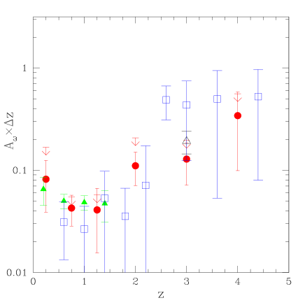
In Figure 6 we compare our values of $A_{\omega}$ (at 10 arcsec) to other published data (Connolly et al. 1998; G98; Magliocchetti & Maddox 1999). The values of $A_{\omega}$ take into account the adopted redshift bin sizes. At a given redshift, a larger $\Delta z$ implies smaller $A_{\omega}$ due to the increasing number of foreground and background galaxies with respect to the unchanged number of physically correlated pairs ($A_{\omega}\propto\Delta z^{-1}$; see e.g. Connolly et al. 1998). Then, if we assume that $A_{\omega}$ does not strongly evolve inside the redshift bin, we can correct the original amplitudes by using $A_{\omega}\times\Delta z$, which allows a more direct comparison. From this figure we note that our results are in good agreement with those of Connolly et al. (1998) and slightly smaller than those for LBGs obtained by G98. The agreement with Magliocchetti & Maddox (1999) is worse but still consistent with both error bars. In this figure we show the possible effect of the contamination factor discussed in the previous section. This correction increases all the values which should be regarded as upper-limits due to the basic assumption that the contaminating population is uncorrelated. Moreover we notice that our estimate in the redshift bin $0\leq z\leq 0.5$ can be affected by the lack of nearby bright galaxies in the HDF. For this reason, this point will be not considered in the following comparison between observational results and model predictions

5 Comparison with theoretical models

5.1 The formalism

We can now predict the behaviour of the angular correlation function $\omega(\theta)$ for our galaxy sample in various cosmological structure formation models. The angular two-point function for a sample extended in the redshift direction over an interval ${\cal Z}$ can be written in terms of the spatial correlation function using the relativistic Limber equation (Peebles 1980). We adopt here the Limber formula as given in Matarrese et al. (1997), namely

$$\omega_{\rm obs}(\theta)=N^{-2}\int_{\cal Z}dz\biggl{(}{dr\over dz}\biggr{)}^{-1}~{}{\cal N}^{2}(z)\int_{-\infty}^{\infty}du~{}\xi_{\rm gal}[r(u,\theta,z),z]\;$$ (4)

where $r(u,\theta,z)=\sqrt{u^{2}+r^{2}(z)\theta^{2}}$, in the small-angle approximation (e.g. Peebles 1980).

The relation between the comoving radial coordinate $r$ and the redshift $z$ is given with whole generality by

$$r(z)={c\over H_{0}\sqrt{|\Omega_{0\cal R}|}}{\cal S}\left(\sqrt{|\Omega_{0\cal R}|}\int_{0}^{z}\left[\left(1+z^{\prime}\right)^{2}\left(1+\Omega_{\rm 0m}z^{\prime}\right)-z^{\prime}\left(2+z^{\prime}\right)\Omega_{0\Lambda}\right]^{-1/2}dz^{\prime}\right)\;,$$ (5)

where $\Omega_{0\cal R}\equiv 1-\Omega_{\rm 0m}-\Omega_{0\Lambda}$, with $\Omega_{\rm 0m}$ and $\Omega_{0\Lambda}$ the density parameters for the non-relativistic matter and cosmological constant components, respectively. In this formula, for an open universe model, $\Omega_{0\cal R}>0$, $S(x)\equiv\sinh(x)$, for a closed universe, $\Omega_{0\cal R}<0$, $S(x)\equiv\sin(x)$, while in the EdS case, $\Omega_{0\cal R}=0$, $S(x)\equiv x$.

In the Limber equation above, ${\cal N}(z)$ is the redshift distribution of the catalogue (whose integral over the entire redshift interval is $N$), which is given by ${\cal N}(z)=\int_{\cal M}d\ln M{\cal N}(z,M)$, with ${\cal N}(z,M)=4\pi g_{c}(z)\phi(z,M)\bar{n}_{c}(z,M)$ and $\bar{n}_{c}(z,M)$ is the expected number of galaxies per comoving volume at redshift $z$; $\phi(z,M)$ is the isotropic catalogue selection function. The quantity ${\cal N}(z,M)$ represents the number of objects actually present in the catalogue, with redshift in the range $z,~{}z+dz$ and intrinsic properties (like mass, luminosity, …) in the range $M,~{}M+dM$ (${\cal M}$ representing the overall interval of variation of $M$). In the latter integral we also defined the comoving Jacobian

$$g_{c}(z)\equiv r^{2}(z)\biggl{[}1+{H_{0}^{2}\over c^{2}}~{}\Omega_{0\cal R}~{}r^{2}(z)\biggr{]}^{-1/2}{dr\over dz}\;.$$ (6)

In what follows we will assume a simple model for our galaxy distribution, where galaxies are associated in a one-to-one correspondence to their hosting dark matter haloes. The advantage of this model is that haloes can be simply characterized by their mass $M$ and formation redshift $z_{f}$. Since haloes merge continuously into larger mass ones one can safely assume that their formation redshift coincides with the observation one, namely $z_{f}=z$. This simple model of galaxy clustering was named ‘transient’ model in Matarrese et al. (1997) and Moscardini et al. (1998); Coles et al. (1998) adopted it to describe the clustering of LBGs. The application of this model is more appropriate at high redshifts where merging dominates while at low redshifts it can only be a rough approximation. Recently Baugh et al. (1999) showed that this simple model under-predicts the clustering properties at low redshift because it does not take into account the possibility that a single halo can host more than one galaxy. Indeed, as discussed in Moscardini et al. (1998), a ‘galaxy conserving’ bias model is likely to provide a better description of the galaxy clustering evolution at low redshift.

In practice, in our modelling we select a minimum mass $M_{\rm min}$ for the haloes hosting our galaxies, i.e. we take $\phi(z,M)=\theta(M-M_{\rm min})$, with $\theta$ the Heaviside step function, and we compute the corresponding value of the effective bias $b_{\rm eff}$ (see equation below) at each redshift. In what follows we will consider two possibilities: i) $M_{\rm min}$ fixed to a sensible value (we will show results obtained by using $10^{10}$, $10^{11}$ and $10^{12}$ $h^{-1}M_{\odot}$), ii) $M_{\rm min}=M_{\rm min}(z)$ chosen to reproduce a relevant set of observational data. For the latter case we will adopt two different strategies: in the first case we assume $M_{\rm min}(z)$ so that the theoretical ${\cal N}(z)$ fits the observed one in each redshift bin (e.g. Mo & Fukugita 1996; Moscardini et al. 1998; A98; Mo, Mao & White 1999); in the second case we adopt at any redshift the median of the mass distribution estimated by our GISSEL model. Actually this model gives a rough estimate of the baryonic mass. To convert it to the mass of the hosting dark matter halo we multiply by a factor 10. This value corresponds to a baryonic fraction close to that predicted by the standard theory of primordial nucleosynthesis. Variations in the range from 5 to 20 produce only small changes in the following results.

As a first, though accurate, approximation the galaxy spatial two-point function can be taken as being linearly proportional to that of the mass, namely $\xi_{\rm gal}(r,z)\simeq b_{\rm eff}^{2}(z)\xi_{\rm m}(r,z)$, where

$$b_{\rm eff}(z)\equiv{\cal N}(z)^{-1}\int_{\cal M}d\ln M^{\prime}~{}{\cal N}(z,M^{\prime})~{}b(M^{\prime},z)$$ (7)

is the effective bias of our galaxy sample and $\xi_{\rm m}$ the matter covariance function.

The bias parameter $b(M,z)$ for haloes of mass $M$ at redshift $z$ in a given cosmological model can be modeled as (Mo & White 1996)

$$b(M,z)=1+{1\over\delta_{c}}\biggl{(}{\delta_{c}^{2}\over\sigma_{M}^{2}D_{+}^{2}(z)}-1\biggr{)}\;,$$ (8)

where $\sigma^{2}_{M}$ is the linear mass-variance averaged over the scale $M$, extrapolated to the present time ($z=0$), $\delta_{c}$ the critical linear overdensity for spherical collapse ($\delta_{c}={\rm const}=1.686$ in the EdS case, while it depends slightly on $z$ for more general cosmologies) and $D_{+}(z)$ is the linear growth factor of density fluctuations (e.g. $D_{+}(z)=(1+z)^{-1}$ in the EdS case). In comparing our theoretical predictions on clustering with the data, we will always adopt for the galaxy redshift distribution ${\cal N}(z)$ the observed one. Nevertheless, consistency requires that the predicted halo redshift distribution for a given minimum halo mass always exceeds (because of the effects of the selection function) the observed galaxy one. For the calculation of the effective bias, where we need ${\cal N}(z,M)$, one might adopt the Press & Schechter (1974) recipe to compute the comoving halo number density (per unit logarithmic interval of mass); it reads

$$\bar{n}_{c}(z,M)=\sqrt{2\over\pi}{{\bar{\varrho}_{0}}\delta_{c}\over MD_{+}(z)\sigma_{M}}\bigg{|}{d\ln\sigma_{M}\over d\ln M}\bigg{|}\exp\biggl{[}-{\delta_{c}^{2}\over 2D_{+}^{2}(z)\sigma^{2}_{M}}\biggr{]}\;$$ (9)

(with $\bar{\varrho}_{0}$ the mean mass density of the Universe at $z=0$).

However, a number of authors have recently shown that the Press-Schechter formula does not provide an accurate description of the halo abundance both in the large and small-mass tails (see e.g. the discussion in Sheth & Tormen 1999). Also, the simple Mo & White (1996) bias formula of Equation (7) has been shown not to correctly reproduce the correlation of low mass haloes in numerical simulations. Several alternative fits have been recently proposed (Jing 1998; Porciani, Catelan & Lacey 1999; Sheth & Tormen 1999; Jing 1999). An accurate description of the abundance and clustering properties of the dark matter haloes corresponding to our galaxy population will be obtained here by adopting the relations introduced by Sheth & Tormen (1999), which have been obtained by fitting to the distribution of the halo population of the GIF simulations (Kauffmann et al. 1999): this technique allows to simultaneously improve the performance of both the mass function and the bias factor. The relevant formulas, replacing Eqs.(8) and (9) above, read

$$b(M,z)=1+{1\over\delta_{c}}\biggl{(}{a\delta_{c}^{2}\over\sigma_{M}^{2}D_{+}^{2}(z)}-1\biggr{)}+{2p\over\delta_{c}}\biggl{(}{1\over{1+[\sqrt{a}\delta_{c}/(\sigma_{M}D_{+}(z))]^{2p}}}\biggr{)}\;$$ (10)

and

$$\bar{n}_{c}(z,M)=\sqrt{2aA^{2}\over\pi}{{\bar{\varrho}_{0}}\delta_{c}\over MD_{+}(z)\sigma_{M}}\biggl{[}1+\biggl{(}{{D_{+}(z)\sigma_{M}}\over{\sqrt{a}\delta_{c}}}\biggr{)}^{2p}\biggr{]}\bigg{|}{d\ln\sigma_{M}\over d\ln M}\bigg{|}\exp\biggl{[}-{a\delta_{c}^{2}\over 2D_{+}^{2}(z)\sigma^{2}_{M}}\biggr{]}\;,$$ (11)

respectively. In these formulas $a=0.707$, $p=0.3$ and $A\approx 0.3222$, while one would recover the standard (Mo & White and Press & Schechter) relations for $a=1$, $p=0$ and $A=1/2$.

The computation of the clustering properties of any class of objects is completed by the specification of the matter covariance function $\xi_{\rm m}(r,z)$ and its redshift evolution. To this purpose we follow Matarrese et al. (1997) and Moscardini et al. (1998) who used an accurate method, based on the Hamilton et al. (1991) original ansatz to evolve $\xi_{\rm m}(r,z)$ into the fully non-linear regime. Specifically, we use here the fitting formulas proposed by Peacock & Dodds (1996).

As recently pointed out by various authors (e.g. Villumsen 1996; Moessner, Jain & Villumsen 1998), when the redshift distribution of faint galaxies is estimated by applying an apparent magnitude limit criterion, magnification bias due to weak gravitational lensing would modify the relation between the intrinsic galaxy spatial correlation function and the observed angular one. Modelling this effect within the present scheme would be highly desirable, but is certainly beyond the scope of our work. Nevertheless, we note that this magnification bias would generally lead to an increase of the apparent clustering of high-$z$ objects above that produced by the intrinsic galaxy correlations, by an amount which depends on the amplitude of the fluctuations of the underlying matter distribution.

5.2 Structure formation models

We will consider here a set of cosmological models belonging to the general class of Cold Dark Matter (CDM) scenarios. The linear power-spectrum for these models can be represented by $P_{\rm lin}(k,0)\propto k^{n}T^{2}(k)$, where we use the fit for the CDM transfer function $T(k)$ given by Bardeen et al. (1986), with “shape parameter” $\Gamma$ defined as in Sugiyama (1995). To fix the amplitude of the power spectrum (generally parameterized in terms of $\sigma_{8}$, the r.m.s. fluctuation amplitude inside a sphere of $8h^{-1}$ Mpc) we either attempt to fit the local cluster abundance, following the Eke, Cole & Frenk (1996) analysis of the temperature distribution of X-ray clusters (Henry & Arnaud 1991), or the level of fluctuations observed by COBE (Bunn & White 1997). In particular, we consider the following models: A version of the standard CDM (SCDM) model with $\sigma_{8}=0.52$, which reproduces the local cluster abundance, but is inconsistent with COBE data. The so-called $\tau$CDM model (White, Gelmini & Silk 1995), with shape parameter $\Gamma=0.21$. A COBE normalized tilted model, hereafter called TCDM (Lucchin & Matarrese 1985), with $n=0.8$, $\sigma_{8}=0.52$ and high (10 per cent) baryonic content (e.g. White et al. 1996; Gheller, Pantano & Moscardini 1998); the normalization of the scalar perturbations, which takes into account the production of gravitational waves predicted by inflationary theories (e.g. Lucchin, Matarrese & Mollerach 1992; Lidsey & Coles 1992), allows to simultaneously fit the CMB fluctuations observed by COBE and the local cluster abundance. The three above models are all flat and without cosmological constant. We also consider here: A cluster normalized open CDM model (OCDM), with matter density parameter $\Omega_{\rm 0m}=0.3$, and $\sigma_{8}=0.87$, which is also consistent with COBE data. Finally, a cluster normalized low-density CDM model ($\Lambda$CDM), with $\Omega_{\rm 0m}=0.3$, but with a flat geometry provided by the cosmological constant, with $\sigma_{8}=0.93$, which is also consistent with COBE data. A summary of the parameters of the cosmological models used here is given in Table 4.

Table 4: The parameters of the cosmological models. Column 2: the present matter density parameter $\Omega_{\rm 0m}$; Column 3: the present cosmological constant contribution to the density $\Omega_{0\Lambda}$; Column 4: the primordial spectral index $n$; Column 5: the Hubble parameter $h$; Column 6: the shape parameter $\Gamma$; Column 7: the spectrum normalization $\sigma_{8}$.

Model	$\Omega_{\rm 0m}$	$\Omega_{0\Lambda}$	$n$	$h$	$\Gamma$	$\sigma_{8}$
SCDM	1.0	0.0	1.0	0.50	0.45	0.52
$\tau$CDM	1.0	0.0	1.0	0.50	0.21	0.52
TCDM	1.0	0.0	0.8	0.50	0.41	0.52
OCDM	0.3	0.0	1.0	0.65	0.21	0.87
$\Lambda$CDM	0.3	0.7	1.0	0.65	0.21	0.93

5.3 Results

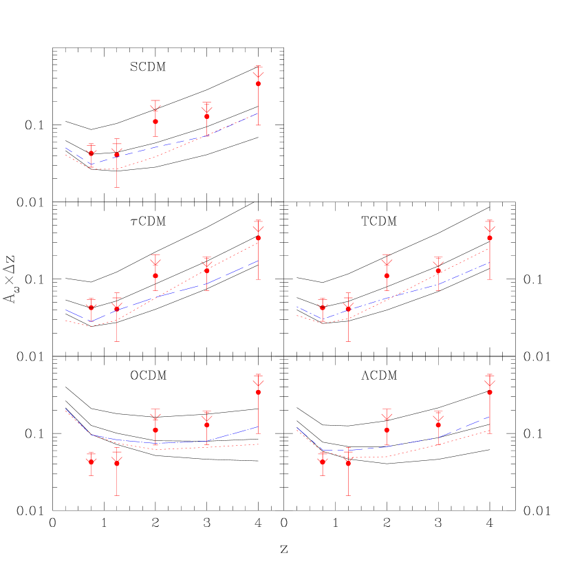
In Figure 7 we compare the observed amplitude of the ACF with the predictions of the various cosmological models. For consistency with the analysis performed on the observational data shown in the previous section, here the theoretical results have been obtained by fitting the data in the same range of angular separation and using the same stepping $\Delta\log\theta=0.3$. A fixed slope of $\delta=0.8$ is also used in the following analysis. Notice that this value is only a rough estimate of the best fit slopes: generally the resulting values are smaller ($\delta\simeq 0.6$) in all redshift intervals and for all the models. The discrepancy is higher for TCDM and $\tau$CDM ($\delta\simeq 0.3-0.4$) and can lead to some ambiguity in the interpretation of the results (see the discussion on the effective bias below).

In each panel the solid lines show the results obtained when we use different (but constant in redshift) values of $M_{\rm min}$ ($10^{10}$, $10^{11}$ and $10^{12}$ $h^{-1}M_{\odot}$ from bottom to top). These results can be regarded as a reference on what is the minimum mass of the galaxies necessary to reproduce the observed clustering strength. However, the assumption that the catalogue samples at any redshift the same class of objects, i.e. with the same typical minimum mass, cannot be realistic. In fact, we expect that at high redshifts the sample tends to select more luminous, and on average more massive, objects than at low redshifts. This is supported by the distribution of the galaxy masses inferred by the GISSEL model, shown in Figure 8. The solid line, which represents the median mass, is an increasing function of redshift: from $z\simeq 0$ to $z\simeq 4$ its value changes by at least a factor of 30. In Figure 8 we also show the masses necessary to reproduce at any redshift the observed galaxy density. In general, they are compatible with the GISSEL distribution but the redshift dependence is different for the various cosmological models considered here. For EdS universe models (left panel) the different curves are quite similar and almost constant with typical values of $10^{10.5}h^{-1}M_{\odot}$. On the contrary for OCDM and $\Lambda$CDM models (shown in the right panel) $M_{\rm min}(z)$ is an increasing function of redshift: at $z\simeq 0$ $M_{\rm min}\simeq 10^{10}h^{-1}M_{\odot}$, while at $z\simeq 4$ $M_{\rm min}\simeq 10^{11.5}h^{-1}M_{\odot}$. The amplitudes of the ACF obtained by adopting these $M_{\rm min}(z)$ values are also shown in Figure 7.

In general, all the models are able to reproduce the qualitative behaviour of the observed clustering amplitudes, i.e. a decrease from $z=0$ to $z\simeq 1-1.5$ and an increase at higher redshifts. The EdS models are in rough agreement with the observational results when a minimum mass of $10^{11}h^{-1}M_{\odot}$ is used at any redshift. As discussed above this mass is slightly larger than the one required to fit the observed ${\cal N}(z)$. The situation for OCDM and $\Lambda$CDM models is different. The amount of clustering measured would require that the involved objects have, at redshifts $z\leq 1-1.5$, minimum masses smaller than $10^{10}h^{-1}M_{\odot}$, at redshifts $1.5\raise-2.0pt\hbox{\hbox to0.0pt{\hbox{$\sim$}\hss}\raise 5.0pt\hbox{$<$}\ }z\raise-2.0pt\hbox{\hbox to0.0pt{\hbox{$\sim$}\hss}\raise 5.0pt\hbox{$<$}\ }3$, minimum masses of the order of $10^{11.5}h^{-1}M_{\odot}$, while, at $z\simeq 4$, $M_{\rm min}\geq 10^{12}h^{-1}M_{\odot}$ is needed to reproduce the clustering strength. These small values at low redshifts are probably due to the kind of biasing model adopted in an epoch when merging starts to be less important. This is particularly true for open models and flat models with a large cosmological constant, where the growth of perturbations is frozen by the rapid expansion of the universe. On the contrary, the need to explain the high amplitude of clustering at $z\simeq 4$ with very massive objects can be in conflict with the observed abundance of galaxies at this redshift, which requires smaller minimum masses.

Figure 7: Comparison of the observed $A_{\omega}$ (filled circles for $I_{AB}\leq 28.5$, arrows for the upper-limits estimates) with the prediction of the various theoretical models described in the text. The solid lines show the measurements expected when a minimum mass $M_{\rm min}=10^{10}$, $10^{11}$ and $10^{12}h^{-1}M_{\odot}$ is assumed; the lower curves refer to smaller masses. The dotted lines show the prediction obtained by using the median masses at any redshift estimated by our GISSEL model shown in Figure 8 (baryonic masses are translated into the masses of the hosting dark matter haloes by multiplying by a factor of 10; see text). The dashed curves correspond to models where the masses necessary to reproduce the observed density of objects in each redshift bin are used. The dashed curve types used for the different cosmological models are the same as those used in Figure 8.

Figure 8: In both panels, the solid line shows, as a function of the redshift, the median of the distribution of the galaxy masses estimated by our GISSEL model; the lower and upper quartiles are shown by dotted lines. The baryonic masses are translated into the masses of the hosting dark matter haloes multiplying by a factor 10. We show also the mass necessary to reproduce the observed density of objects at any $z$ for SCDM (short-dashed line), $\tau$CDM (long-dashed line) and TCDM (short-dashed – dotted line) models in the left panel and for OCDM (long-dashed – dotted line) and $\Lambda$CDM (long-dashed – short–dashed line) models in the right panel.

If the spatial correlation function can be written in the simple form $\xi_{\rm gal}(r,z)=[r/r_{0}(z)]^{-\gamma}$, it is possible to obtain the comoving correlation length $r_{0}(z)$ and the r.m.s. galaxy density fluctuation $\sigma^{\rm gal}_{8}(z)$, with the assumption that the clustering does not strongly evolve inside each redshift bin used for the amplitude measurements (see Magliocchetti & Maddox 1999 for the relevant formulas in the framework of different cosmological models).

The values for the comoving $r_{0}(z)$ obtained from our data are listed in Table 5 for three different cosmologies. In Figure 9, we compare our values of $r_{0}$ as a function of $z$ to a compilation of values taken from the literature. The results are given under the assumption of an EdS universe. From this figure, one can notice that $r_{0}$ shows a small decline from $z\simeq 0$ to $z\simeq 1-1.5$ followed by an increase at higher $z$. At $z\geq 2$ the clustering amplitude is comparable to or higher than that observed at $z\simeq 0.25$.

Table 5: The amplitude of $\omega(\theta)$ at 10 arcsec ($A_{\omega}$) for different redshift bins with $I_{AB}\leq 28.5$. Column 1: the redshift range. Column 2: the number of galaxies in the redshift bin. Column 3: the amplitude of the ACF at 10 arcsec. Columns 4, 5, 6: the comoving correlation length $r_{0}$ (in $h^{-1}$ Mpc) as derived from the Limber equation for three different cosmological models (EdS model, open model with $\Omega_{\rm 0m}=0.3$ and a flat model with $\Omega_{\rm 0m}=0.3$ and cosmological constant). All the listed values are not corrected for the contamination.

$z$ range	Number of	$A_{\omega}$	$r_{0}$	$r_{0}$	$r_{0}$
	galaxies	(at 10 arcsec)	$\Omega_{\rm 0m}=1,\Omega_{\rm 0\Lambda}=0$	$\Omega_{\rm 0m}=0.3,\Omega_{\rm 0\Lambda}=0$	$\Omega_{\rm 0m}=0.3,\Omega_{\rm 0\Lambda}=0.7$
0.0 - 0.5	96	0.17 $\pm$ 0.09	1.63 $\pm$ 0.47	1.77 $\pm$ 0.51	1.93 $\pm$ 0.56
0.5 - 1.0	294	0.09 $\pm$ 0.03	1.37 $\pm$ 0.25	1.69 $\pm$ 0.31	1.93 $\pm$ 0.36
1.0 - 1.5	157	0.09 $\pm$ 0.05	1.21 $\pm$ 0.41	1.64 $\pm$ 0.56	1.82 $\pm$ 0.63
1.5 - 2.5	202	0.12 $\pm$ 0.04	1.92 $\pm$ 0.38	3.06 $\pm$ 0.61	3.07 $\pm$ 0.61
2.5 - 3.5	142	0.13 $\pm$ 0.06	1.69 $\pm$ 0.41	3.06 $\pm$ 0.75	2.78 $\pm$ 0.68
3.5 - 4.5	35	0.35 $\pm$ 0.25	2.56 $\pm$ 1.01	5.29 $\pm$ 2.08	4.28 $\pm$ 1.69
0.0 - 6.0	959	0.03 $\pm$ 0.01

Figure 9: The measured comoving correlation length $r_{0}(z)$ (in $h^{-1}$ Mpc) as obtained from the values of $A_{\omega}$ by assuming an EdS universe (filled circles; the arrows refer to the upper-limits due to the contamination). Previous determinations are shown by the same symbols as in Figure 6. We add also the values obtained from the analysis of the CFRS (Le Fèvre et al. 1996; cross symbols), from the count-in-cell analysis of the LBG catalogue (Adelberger et al. 1998; filled triangle) and the local values obtained from the APM survey (Loveday et al. 1995; full sample, E/S0 and Sp/Irr sub-samples are shown by the filled square, and the high and low open squares, respectively). The curves show the evolution of the clustering using the $\epsilon$ model with three values of the parameter $\epsilon$: $\epsilon=0.8$ (linear growth of clustering, solid line); $\epsilon=2$ (growth more rapid than the linear prediction, dotted line), $\epsilon=-1.2$ (fixed clustering in comoving coordinates, dashed line). The curves have been arbitrarily scaled to our observed value at $z=0.75$.

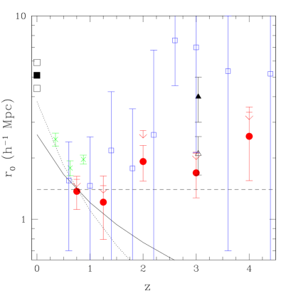
An implication of the results shown in this figure is that the evolution of galaxy clustering cannot be properly described by the standard parametric form: $\xi(r,z)=\xi(r,z=0)\ (1+z)^{-(3+\epsilon-\gamma)}$, where $\epsilon$ models the gravitational evolution of the structures. Due to the dependence of the bias on redshift and mass, the evolution of galaxy clustering is related to the clustering of the mass in a complex way. This has already been noticed by G98 from the study of LBGs at $z\simeq 3$ (see also Moscardini et al. 1998 for a theoretical discussion of the problem).

In the plot of the correlation length $r_{0}$ we present also the results for $z<1$ obtained by Le Fèvre et al. (1996) from the estimates of the projected correlation function of the CFRS. We do not show in the figure the correlation lengths obtained by Carlberg et al. (1997), who performed the same analysis using a K selected sample, because they adopted a different cosmological model. Their estimates with $q_{0}=0.1$ of $r_{0}$ are approximately a factor of 1.5 larger than the CFRS results in a comparable magnitude and redshift range. Our results are lower than these previous estimates and show that the objects selected by our catalogue at low redshifts tend to have different clustering properties. This effect suggests a dependence of the clustering properties on the selection of the sample which is even more evident at high redshift. In fact our value of $r_{0}$ at $z\simeq 3$ is smaller than that obtained by A98 and G98 for their LBG catalogues at the same redshift. To measure the clustering properties, A98 used a bright sample of 268 spectroscopically confirmed galaxies and derived $r_{0}\simeq 4\ h^{-1}$ Mpc; G98 used a larger sample of 871 galaxies and derived a value two times smaller ($r_{0}\simeq 2\ h^{-1}$ Mpc). Our value, referring to galaxies with $I_{AB}\leq 28.5$, is $r_{0}\simeq 1.7\ h^{-1}$ Mpc. Notice that this value is a lower limit since it does not take into account the effects of contamination. All these reported values of the correlation length are obtained by assuming an EdS universe. This decrease of $r_{0}$ suggests that at fainter magnitudes we observe less massive galaxies which are intrinsically less correlated. This is in qualitative agreement with the prediction of the hierarchical galaxy formation scenario (e.g. Mo, Mao & White 1999). On the contrary, such an interpretation is only marginally consistent with the reported higher value at $z\simeq 3$ of Magliocchetti & Maddox (1999), computed with the same FLY99 catalogue.

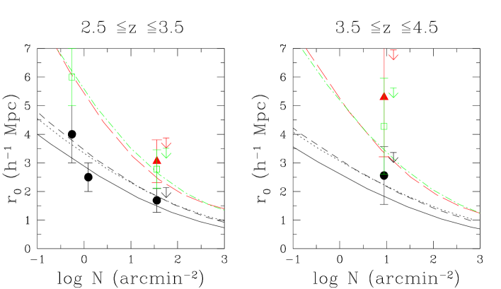
In order to better display the relation between the clustering strength and the abundance of a given class of objects (defined as haloes with mass larger than a given mass $M_{\rm min}$) in Figure 10 we show, for the different cosmological models, the relation between the predicted correlation length $r_{0}$ and the expected surface density, i.e. the number of objects per square arcminute. The quantity $r_{0}$ shown in this figure is defined as the comoving separation where the predicted spatial correlation is unity; the number density is computed by suitably integrating the modified Press-Schechter formula [Equation (11)] over the given redshift range. In the left panel, showing the results for the interval $2.5\leq z\leq 3.5$, we also plot the results obtained in this work (points at high density with their associated upper-limits due to contamination effects) and those coming from the LBG analysis of A98 and G98 and corresponding to a lower abundance. All the models are able to reproduce the observed scaling of the clustering length with the abundance and no discrimination can be made between them. Similar conclusions have been reached by Mo, Mao & White (1999). The right panel shows the same plot but at $z\simeq 4$, where the only observational estimates come from this work and from Magliocchetti & Maddox (1999). Here the situation seems to be more interesting. In fact the observed clustering is quite high and in the framework of the hierarchical models seems to require a low abundance for the relevant objects. This density starts to be in conflict with the observed one (which represents a lower limit due to the unknown effect of the selection function) for some of the models here considered, for example the OCDM model. Thus, if our results will be confirmed by future observations, the combination of the clustering strength and galaxy abundance at redshift $z\simeq 4$ could be a discriminant test for the cosmological parameters.

Figure 10: The comoving correlation length $r_{0}$ (in $h^{-1}$ Mpc) as a function of surface density (defined as the expected number of objects per square arcminute) in two different redshift intervals: $2.5\leq z\leq 3.5$ (left panel) and $3.5\leq z\leq 4.5$ (right panel). Different lines refer to the predictions of various cosmological models: SCDM (solid lines), $\tau$CDM model (short-dashed lines), TCDM (dotted lines), OCDM(long-dashed lines) and $\Lambda$CDM (dotted-dashed lines). For comparison we show (at $\log N\simeq 1.55$ in the left panel and at $\log N\simeq 0.95$ in the right panel) the results obtained in this work for three cosmologies: filled circle, filled triangle and open square refer to EdS models, open and flat universe with cosmological constant, respectively. The arrows refer to the upper-limits due to contamination effects and are shifted of 0.2 in abscissa for clarity. In the left panel we show also the results obtained from the analysis of the LBG clustering by Adelberger et al. (at $\log N\simeq-0.26$, for Einstein-de Sitter universe and for flat universe with cosmological constant), and from Giavalisco et al. (at $\log N\simeq 0.09$, only for EdS model).

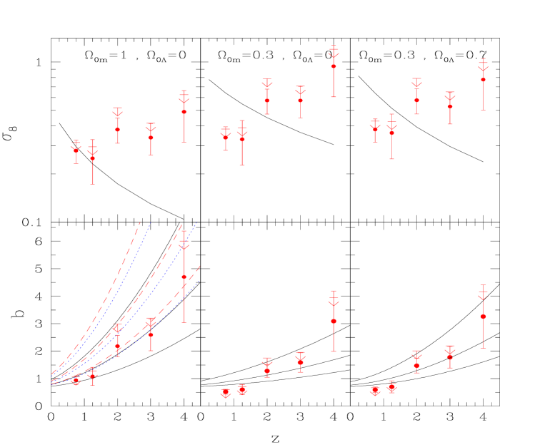
An alternative way to study the clustering properties is given by the observed r.m.s. galaxy density fluctuation $\sigma_{8}^{\rm gal}$. Its redshift evolution is shown in the upper panels of Figure 11 for three cosmological models: Einstein-de Sitter universe (left panel); open universe with $\Omega_{\rm 0m}=0.3$ and vanishing cosmological constant (central panel); flat universe with $\Omega_{\rm 0m}=0.3$ and cosmological constant (right panel). In the same plot we show also the theoretical predictions computed by using the linear theory when the cosmological models are normalized to reproduce the local cluster abundance. Since the corresponding values of $\sigma_{8}^{\rm m}$ at $z=0$ (reported in Table 4) are smaller than unity, we can safely compute the redshift evolution by adopting linear theory. As shown in Moscardini et al. (1998), the differences between these estimates and those obtained by using the fully non-linear method described above are always smaller than 3% at $z=0$ and consequently negligible at higher redshifts. The comparison suggests that, while some anti-bias is present at low redshift, the high-redshift galaxies are strongly biased with respect to the dark matter. This observation strongly supports the theoretical expectation of biased galaxy formation with a bias parameter evolving with $z$.

Finally, the lower panels of Figure 11 report directly the values of the bias parameter $b$ as deduced from our catalogue. The results show that $b$ is a strongly increasing function of redshift in all cosmological models: from $z\simeq 0$ to $z\simeq 4$ the bias changes from $b\simeq 1$ to $b\simeq 5$ in the EdS model and from $b\simeq 0.5$ to $b\simeq 3$ in OCDM and $\Lambda$CDM models. This qualitative behaviour is what is expected in the framework of the hierarchical models of galaxy formation, as confirmed by the curves of the effective bias computed by using Equation (7), with $M_{\rm min}=10^{10}$, $10^{11}$ and $10^{12}h^{-1}M_{\odot}$. The observed bias is well reproduced when a minimum mass of $\simeq 10^{11}h^{-1}M_{\odot}$ is adopted for SCDM, in agreement with the discussion of the results about the correlation amplitude $A_{\omega}$. On the contrary, the study of the bias parameter for the other two EdS models (TCDM and $\tau CDM$) seems to suggest a smaller value of $M_{\rm min}\simeq 10^{10}h^{-1}M_{\odot}$. The discrepancy is due to the fact that the computation of the correlation amplitudes has been made by adopting a fixed slope of $\delta=0.8$, which is not a good estimate of the best fit value for these two models. For OCDM and $\Lambda$CDM models a minimum mass of $M_{\rm min}\simeq 10^{11}h^{-1}M_{\odot}$ gives an effective bias in agreement with the observations when $1.5\raise-2.0pt\hbox{\hbox to0.0pt{\hbox{$\sim$}\hss}\raise 5.0pt\hbox{$<$}\ }z\raise-2.0pt\hbox{\hbox to0.0pt{\hbox{$\sim$}\hss}\raise 5.0pt\hbox{$<$}\ }3$, while a smaller (larger) minimum mass is required at lower (higher) redshifts.

Figure 11: The upper panels show (data as filled circles and upper-limits as arrows) our observed r.m.s. galaxy density fluctuation $\sigma_{8}^{\rm gal}(z)$ for three cosmologies (left: EdS universe; middle: open universe with $\Omega_{\rm 0m}=0.3$ and vanishing cosmological constant; right: flat universe with $\Omega_{\rm 0m}=0.3$ and cosmological constant). The solid lines show the r.m.s. mass density fluctuation $\sigma_{8}^{\rm m}(z)$ for the same cosmologies, as obtained by linear theory. The models are normalized to reproduce the local abundance of the galaxy clusters. The lower panels show the measured bias $b$ as a function of redshift [with $b(z)\equiv\sigma_{8}^{\rm gal}(z)/\sigma_{8}^{\rm m}(z)$]. The curves show, for different cosmological models, the theoretical effective bias computed with different values of minimum mass. For the EdS universe three cosmological models are shown in the left panel: SCDM (solid lines), $\tau$CDM (dashed lines) and TCDM (dotted lines). The central and right panels refer to OCDM and $\Lambda$CDM models, respectively. We show results for $M_{\rm min}=10^{10}$, $10^{11}$ and $10^{12}h^{-1}M_{\odot}$ (lower curves are for smaller masses).

We can analyze the properties of the present-day descendants of our galaxies at high $z$, assuming that the large majority of them contains only one of our high-redshift galaxies (see e.g. Baugh et al. 1998). Following Mo, Mao & White (1999), we can obtain the present bias factor of these descendants by evolving $b(z)$ backwards in redshift from the formation redshift $z$ to $z=0$, according to the ‘galaxy-conserving’ model (Matarrese et al. 1997; Moscardini et al. 1998); this gives

$$b(M,0)=1+D_{+}(z)\bigl{[}b(M,z)-1\bigr{]}\;,$$ (12)

where, for $b(M,z)$, we can use the effective bias obtained for our galaxies by dividing the observed galaxy r.m.s. fluctuation on $8~{}h^{-1}$ Mpc by that of the mass, which depends on the background cosmology. For the galaxies at $z\simeq 3$ we find $b(M,0)\simeq 1.4,1.3,1.3$ for the EdS, OCDM and $\Lambda$CDM models, respectively. The values of $b(M,0)$ that we obtained can be directly compared with those for normal bright galaxies, which have $b_{0}\approx 1/\sigma_{8}$, i.e. approximately 1.9 in the EdS universe and 1.1 in the OCDM and $\Lambda$CDM models. Consequently, the descendants of our galaxies at $z\simeq 3$ appear in the EdS universe to be less clustered than the present-day bright galaxies and can be found among field galaxies. On the contrary, the values resulting for the OCDM and $\Lambda$CDM models seem to imply that the descendants are clustered at least as much as the present-day bright galaxies, so they could be found among the brightest galaxies or inside clusters. This is in agreement with the findings of Mo, Mao & White (1999) for the LBGs (see also Mo & Fukugita 1996; Governato et al. 1998; Baugh et al. 1999). If we repeat the analysis by using our galaxies at redshift $z\simeq 4$, we find that $b(M,0)\simeq 1.8,1.7,1.6$ for the EdS, OCDM and $\Lambda$CDM models, respectively. The ratio between the correlation amplitudes of the descendants and the normal bright galaxies is $\simeq 0.9,2.3,2.2$. This result confirms that for the EdS models they have clustering properties comparable to “normal” galaxies, while for non-EdS models the descendants seem to be very bright and massive galaxies.

6 Discussion and Conclusions

In this paper we have measured over the redshift range $0\leq z\leq 4.5$ the clustering properties of a faint galaxy sample in the HDF North (Fernández-Soto et al. 1999), by using photometric redshift estimates. This technique makes it possible both to isolate galaxies in relatively narrow redshift intervals, reducing the dilution of the clustering signal (in comparison with magnitude limited samples; Villumsen, Freudling & da Costa 1997), and to measure the clustering evolution over a very large redshift interval for galaxies fainter than the spectroscopic limits. The comparison with spectroscopic measurements shows that, for galaxies brighter than $I_{AB}\leq 26$, our accuracy is close to $\sigma_{z}\sim 0.1$ for $z\leq 1.5$ and $\sigma_{z}\sim 0.2$ for $z\geq 1.5$. We have checked the reliability of our photometric redshifts in the critical interval $1.2\leq z\leq 2$ by replacing the J, H, Ks photometry of Dickinson et al. (1999) with the $F110W$, $F160W$ measurements in the HDF-N sub-area observed with NICMOS (Thompson et al. 1999). The new photometry is in general consistent with the IR photometry of Fernández-Soto et al. (1999) and our photometric redshifts are not significantly changed. In order to infer the confidence level for the galaxies beyond the spectroscopic limits ($26\leq I_{AB}\leq 28.5$), we have compared our results first with those obtained by other photometric codes and second with Monte Carlo simulations. The first comparison shows that the resulting dispersion is $\sigma_{z}\simeq 0.20$ at $z\leq 1.5$ and increases at higher redshifts ($\sigma_{z}\simeq 0.30$), with a possible systematic shift ($\langle z_{\rm GIS}-z_{\rm CE}\rangle\simeq-0.15$ and $\langle z_{\rm GIS}-z_{\rm FLY99}\rangle\simeq+0.3$). The second comparison with Monte Carlo simulations (made to determine the effects of photometric errors in the redshift estimates) shows that the r.m.s. dispersion obtained in this way is compatible with the previous estimates done by comparing the different codes: for galaxies with $I_{AB}\leq 28.5$ we found $\sigma_{z}\simeq 0.2-0.3$ with a maximum $\sigma_{z}=0.35$ for the redshift range $1.5\leq z\leq 2.5$. The contamination fraction of simulated galaxies incorrectly put in a bin different from the original one due to photometric errors is close to $\sim 20\%$. The dominant source of contamination in a given redshift bin is due to the r.m.s. dispersion in the redshift estimates, with the exception of the bin $0\leq z\leq 0.5$ where the contamination is due to the high-redshift galaxies ($z\geq 1$) improperly put at low $z$. Due to the contamination effect at any redshift, we note that our clustering measurements should be considered as a lower limit. Assuming that the contaminating population is uncorrelated, we have applied a correction $(1-f)^{2}$ to our original measurements, where $f$ is the contaminating fraction. This correction should be regarded as an upper-limit.

As a consequence of the redshift uncertainties we have chosen to compute the angular correlation function $\omega(\theta)$ in large bins with $\Delta z=0.5$ at $z\leq 1.5$ and $\Delta z=1.0$ at $z\geq 1.5$. The resulting $\omega(\theta)$ has been fitted with a standard power-law relation with fixed slope, $\delta=0.8$. This latter value can be questioned because of the present lack of knowledge about the redshift evolution of the slope and its dependence on the different classes of objects. In order to avoid systematic biases in the analysis of the results, the theoretical predictions have been treated with the same basic assumptions. The behaviour of the amplitude of the angular correlation function at 10 arcsec ($A_{\omega}$) shows a decrease up to $z\simeq 1-1.5$, followed by a slow increase. The comoving correlation length $r_{0}$ computed from the clustering amplitudes shows a similar trend but its value depends on the cosmological parameters. Finally, we have compared our $\sigma^{\rm gal}_{8}$ to that of the mass predicted for three cosmologies to estimate the bias. For all cases, we found that the bias is an increasing function of redshift with $b(z\simeq 0)\simeq 1$ and $b(z\simeq 4)\simeq 5$ (for EdS universe), and $b(z\simeq 0)\simeq 0.5$ and $b(z\simeq 4)\simeq 3$ (for open and $\Lambda$ universe). This result confirms and extends in redshift the results obtained by Adelberger et al. (1998) and Giavalisco et al. (1998) for a Lyman-Break galaxy catalogue at $z\simeq 3$, suggesting that these high-redshift galaxies are located preferentially in the rarer and denser peaks of the underlying matter density field.

We have compared our results with the theoretical predictions of a set of different cosmological models belonging to the class of the CDM scenario. With the exception of the SCDM model, all the other models are consistent with both the local observations and the COBE measurements. We model the bias by assuming that the galaxies are associated in a one-to-one correspondence with their hosting dark matter haloes defined by a minimum mass ($M_{\rm min}$). Moreover, we assume that the haloes continuously merge into more massive ones. The values of $M_{\rm min}(z)$ used in these computations refer either to a fixed mass or to the median mass derived by our GISSEL model or to the value required to reproduce the observed density of galaxies at any redshift.

The comparison shows that all galaxy formation models presented in this work can reproduce the redshift evolution of the observed bias and correlation strength. The halo masses required to match the observations depend on the adopted background cosmology. For the EdS universe, the SCDM model reproduces the observed measurements if a typical minimum mass of $10^{11}h^{-1}\ M_{\odot}$ is used, while the $\tau$CDM and TCDM models require a lower typical mass of $10^{10}-10^{10.5}h^{-1}\ M_{\odot}$. For OCDM and $\Lambda$CDM models, the mass is a function of redshift, with $M_{\rm min}\leq 10^{10}h^{-1}\ M_{\odot}$ at $z\leq 1.5$, $10^{11.5}h^{-1}\ M_{\odot}$ between $1.5\leq z\leq 3$ and $10^{12}h^{-1}\ M_{\odot}$ at $z\simeq 4$. The higher masses required at high $z$ to reproduce the clustering strength for these models are a consequence of the smaller bias they predict at high redshifts compared to the EdS models.

We notice that at very low $z$, both OCDM and $\Lambda$CDM models overpredict the clustering and consequently the bias. Two effects may be responsible for this failure. First, the one-to-one correspondence between haloes and galaxies may be an inappropriate description at low $z$, where a more complex picture might be required. Second, we have assumed that merging continues to be effective at low $z$ when, on the contrary, the fast expansion of the universe acts against this process, particularly for these models.

As a consequence of the bias dependence on the redshift and on the selection criteria of the samples, the behaviour of the galaxy clustering cannot provide a straightforward prediction on the behaviour of the underlying matter clustering. For this reason, the parametric form $\xi(r,z)=\xi(r,z=0)(1+z)^{-(3+\epsilon-\gamma)}$, where $\epsilon$ models the gravitational evolution of the structures, cannot correctly describe the observations for any value of $\epsilon$.

Another prediction of the hierarchical models is the dependence of the clustering strength on the limiting magnitude of the samples. At $z\simeq 3$, we have compared our clustering measurements with the previous results obtained for the LBGs by Adelberger et al. (1998) and Giavalisco et al. (1998). The three samples correspond to different galaxy densities (our density in the HDF is approximately 65 times higher than the LBGs of Adelberger et al. 1998). The clustering strength shows a decrease with the density. This result is in excellent agreement (both qualitatively and quantitatively) with the clustering strength predicted by the hierarchical models as a function of the halo density. More abundant haloes are less clustered than less abundant ones (see also Mo et al. 1998). Moreover, this result, which is independent of the adopted cosmology, supports our assumption of a one-to-one correspondence between haloes and galaxies at high-redshifts (see also Baugh et al. 1999), because otherwise we would expect a higher small-scale clustering at the observed density. As also noticed by Adelberger et al. (1998) for LBGs, such a result seems to be incompatible with a model which assumes a stochastic star formation process, which would predict that observable galaxies have a wider range of masses. In fact, in this case the correlation strength should be lower than the observed one because of the contribution by the most abundant haloes (which are less clustered). Moreover, it seems possible to exclude that a very large fraction (more than 50%) of massive galaxies are lost by observations due to dust obscuration, because the correlation strength would be incompatible with the observed density. Consequently, one of the main results of Adelberger et al. (1998), namely the existence of a strong relation between the halo mass and the absolute UV luminosity due to the fact that more massive haloes host the brighter galaxies, seems to be supported by the present work also for galaxies ten times fainter.

We have estimated the clustering properties at the present epoch of the descendants of our high-redshift galaxies. To do so, we have assumed that only one galaxy is hosted by the descendants. The resulting local bias for the descendants of the galaxies at $z\simeq 3$ is $b(z=0)\simeq 1.4,1.3,1.3$ for the EdS, OCDM and $\Lambda$CDM models, respectively. Considering the galaxies at $z\simeq 4$, we obtain $b(z=0)=1.8,1.7,1.6$, respectively. These values seem to indicate that in the case of the the EdS universe they are field or normal bright galaxies while for the OCDM and $\Lambda$CDM models the descendants can be found among the brightest and most massive galaxies (preferentially inside clusters). As already noted, at $z\simeq 3$, the clustering strength and the observed density of galaxies are in good agreement with the theoretical predictions for any fashionable cosmological model. At $z\simeq 4$, the present analysis seems to be more discriminant. Although our estimation should be regarded as tentative and needs future confirmation, we find a remarkably high correlation strength. For some models the observed density of galaxies starts to be inconsistent with the required theoretical halo density. The relation between clustering properties and number density of very high redshift galaxies therefore provides an interesting way to investigate the cosmological parameters. The difference in the predicted masses ($\simeq$ 15 to 30 at $z\simeq$ 3 and 4) between EdS and non-EdS universe models is also in principle testable in terms of measured velocity dispersions. The present results have been obtained in a relatively small field for which the effects of cosmic variance may be important (see Steidel 1998 for a discussion). Nevertheless they show a possibility of challenging cosmological parameters which becomes particularly exciting in view of the rapidly growing wealth of multi-wavelength photometric databases in various deep fields and availability of 10m-class telescopes for spectroscopic follow-up in the optical and near infrared.

References

- [] Abraham R.G., Tanvir N.R., Santiago B.X., Ellis R.S., Glazebrook K., van den Bergh S., 1996, MNRAS, 279, L47
- [] Adelberger K.L., Steidel C.C., Giavalisco M., Dickinson M.E., Pettini M., Kellogg M., 1998, ApJ, 505, 18 (A98)
- [] Bardeen J.M., Bond J.R., Kaiser N., Szalay A.S., 1986, ApJ, 304, 15
- [] Baugh C.M., Benson A.J., Cole S., Frenk C.S., Lacey C.G., 1999, MNRAS, 305, L21
- [] Baugh C.M., Cole S., Frenk C.S., Lacey C.G., 1998, ApJ, 498, 504
- [] Benítez N., 1998, preprint, astro-ph/9811189
- [] Benoist C., Maurogordato S., da Costa L.N., Cappi A., Schaeffer R., 1996, ApJ, 472, 452
- [] Bertin E., Arnouts S., 1996, A&AS, 117, 393
- [] Bruzual G., Charlot S., 1999, in preparation
- [] Bunn E.F., White M., 1997, ApJ, 480, 6
- [] Calzetti D., 1997, in Waller W.H. et al. eds., The Ultraviolet Universe at Low and High Redshift: Probing the Progress of Galaxy Evolution, AIP Conf. Proc. 408. AIP, Woodbury, 403
- [] Calzetti D., Kinney A.L., Storchi-Bregmann T., 1994, ApJ, 429, 582
- [] Carlberg R.G., Cowie L.L., Songaila A., Hu E.M., 1997, ApJ, 484, 538
- [] Coleman G.D., Wu C.C., Weedman D.W., 1980, ApJS, 43, 393
- [] Coles P., Lucchin F., Matarrese S., Moscardini L., 1998, MNRAS, 300, 183
- [] Colín P., Carlberg R.G., Couchman H.M.P., 1997, ApJ, 490, 1
- [] Colombi S., Szapudi I., Szalay A.S., 1998, MNRAS, 296, 253
- [] Connolly A.J., Csabai I., Szalay A.S., Koo D.C., Kron R.G., 1995, AJ, 110, 2655
- [] Connolly A.J., Szalay A.S., Brunner R.J., 1998, ApJ, 499, L125
- [] Dickinson M.E. et al., 1999, in preparation
- [] Eke V.R., Cole S., Frenk C.S., 1996, MNRAS, 282, 263
- [] Fasano G., Cristiani S., Arnouts S., Filippi M., 1998, AJ, 115, 1400
- [] Fernández-Soto A., Lanzetta K.M., Yahil A., 1999, ApJ, 513, 34 (FLY99)
- [] Franceschini A., Silva L., Fasano G., Granato G.L., Bressan A., Arnouts S., Danese L., 1998, ApJ, 506, 600
- [] Gheller C., Pantano O., Moscardini L., 1998, MNRAS, 296, 85
- [] Giallongo E., D’Odorico S., Fontana A., Cristiani S., Egami E., Hu E., McMahon R.G., 1998, AJ, 115, 2169
- [] Giavalisco M., Steidel C.C., Adelberger K.L., Dickinson M.E., Pettini M., Kellogg M., 1998, ApJ, 503, 543 (G98)
- [] Governato F., Baugh C.M., Frenk C. S., Cole S., Lacey C.G., Quinn T., Stadel J., 1998, Nat, 392, 359
- [] Gwyn S.D.J., Hartwick F.D.A., 1996, ApJ, 468, L77
- [] Hamilton A.J.S., Kumar P., Lu E., Mathews A., 1991, ApJ, 374, L1
- [] Henry J.P., Arnaud K.A., 1991, ApJ, 372, 410
- [] Hogg D.W. et al., 1998, AJ, 115, 1418
- [] Jing Y.P., 1998, ApJ, 503, L9
- [] Jing Y.P., 1999, ApJ, 515, L45
- [] Kaiser N., 1984, ApJ, 284, L9
- [] Kauffmann G., Colberg J.M., Diaferio A., White S.D.M., 1999, MNRAS, 303, 188
- [] Kinney A.L., Bohlin R.C., Calzetti D., Panagia N., Wyse R.F.G., 1993, ApJS, 86, 5
- [] Landy S.D., Szalay A.S., 1993, ApJ, 412, 64
- [] Lanzetta K.M., Yahil A., Fernández-Soto A., 1996, Nat, 381, 759
- [] Le Fèvre O., Hudon D., Lilly S.J., Crampton D., Hammer F., Tresse L., 1996, ApJ, 461, 534
- [] Lidsey J.E., Coles P., 1992, MNRAS, 258, L57
- [] Loveday J., Maddox S.J., Efstathiou G., Peterson B.A., 1995, ApJ, 442, 457
- [] Lucchin F., Matarrese S., 1985, Phys. Rev., D32, 1316
- [] Lucchin F., Matarrese S., Mollerach S., 1992, ApJ, 401, L49
- [1] Madau P., 1995, ApJ, 441, 18
- [2] Madau P., Ferguson H.C., Dickinson M.E., Giavalisco M., Steidel C.C., Fruchter A., 1996, MNRAS, 283, 1388
- [] Magliocchetti M., Maddox S.J., 1999, MNRAS, in press, astro-ph/9811320
- [] Matarrese S., Coles P., Lucchin F., Moscardini L., 1997, MNRAS, 286, 115
- [] Miralles J.M., Pelló R., 1998, preprint, astro-ph/9801062
- [] Mo H.J., Fukugita M., 1996, ApJ, 467, L9
- [] Mo H.J., Mao S., White S.D.M., 1999, MNRAS, 304, 175
- [] Mo H.J., White S.D.M., 1996, MNRAS, 282, 347
- [] Moessner R., Jain B., Villumsen J.V., 1998, MNRAS, 294, 291
- [] Moscardini L., Coles P., Lucchin F., Matarrese S., 1998, MNRAS, 299, 95
- [] Park C., Vogeley M.S., Geller M.J., Huchra J.P., 1994, ApJ, 431, 569
- [] Peacock J.A., Dodds S.J., 1996, MNRAS, 280, L19
- [] Peebles P.J.E., 1980, The large–scale structure of the Universe. Princeton University Press, Princeton
- [] Porciani C., Catelan P., Lacey C., 1999, ApJ, 513, L99
- [] Postman M., Lauer T.R., Szapudi I., Oegerle W., 1998, ApJ, 506, 33
- [] Press W.H., Schechter P., 1974, ApJ, 187, 425
- [] Roukema B.F., Valls-Gabaud D., Mobasher B., Bajtlik S., 1999, MNRAS, 305, 151
- [] Santiago B.X., da Costa L.N., 1990, ApJ, 362, 386
- [] Sawicki M.J., Lin H., Yee H.K.C., 1997, AJ, 113, 1 (SLY97)
- [] Sheth R.K., Tormen G., 1999, MNRAS, in press, astro-ph/9901122
- [] Steidel C., 1998, in Banday A.J., Sheth R.K. & L.N. da Costa eds., Proc. of MPA/ESO Conference on Evolution of Large Scale Structure: from Recombination to Garching, in press, astro-ph/9811400
- [] Steidel C., Giavalisco M., Pettini M., Dickinson M.E., Adelberger K., 1996, ApJ, 462, L17
- [] Sugiyama N., 1995, ApJS, 100, 281
- [] Thompson R.I., Storrie-Lombardi L.J., Weymann R.J., Rieke M.J., Schneider G., Stobie E., Lytle D., 1999, AJ, 117, 17
- [] Tucker D.L. et al., 1997, MNRAS, 285, 5
- [] van den Bergh S., Abraham R.G., Ellis R.S., Tanvir N.R., Santiago B.X., Glazebrook K., 1996, AJ, 112, 359
- [] Villumsen J.V., 1996, MNRAS, 281, 369
- [] Villumsen J.V., Freudling W., da Costa L.N., 1997, ApJ, 481, 578
- [] Wang Y., Bahcall N., Turner E.L., 1998, AJ, 116, 2081
- [] White M., Gelmini G., Silk J., 1995, Phys. Rev., D51, 2669
- [] White M., Viana P.T.P., Liddle A.R., Scott D., 1996, MNRAS, 283, 107
- [] Williams R.E. et al., 1996, AJ, 112, 1335