Cosmological Perturbations from the No Boundary Euclidean Path Integral

Abstract

We compute, from first principles, the quantum fluctuations about instanton saddle points of the Euclidean path integral for Einstein gravity coupled to a scalar field. The Euclidean two-point correlator is analytically continued into the Lorentzian region where it describes the quantum mechanical vacuum fluctuations in the state described by no boundary proposal initial conditions. We concentrate on the density perturbations in open inflationary universes produced from cosmological instantons, describing the differences between non-singular Coleman–De Luccia and singular Hawking–Turok instantons. We show how the Euclidean path integral uniquely specifies the fluctuations in both cases.

I Introduction

The idea that the early universe underwent a period of accelerating expansion i.e. inflation, is an attractive one. Such a period of inflation would explain the observed smoothness and flatness of today’s universe. But it might also explain the inhomogeneities present in the universe. During inflation, quantum mechanical vacuum fluctuations in various fields would have been amplified and stretched to macroscopic length scales, to later seed the growth of large scale structures like those we see today.

However, the theoretical foundations of inflation are still unclear. There is no compelling connection between the field needed to drive inflation and fundamental theory. The initial conditions are usually imposed by hand, or via a somewhat handwaving appeal to primordial chaos. The problem of the initial singularity is not addressed. And the usual calculation of the quantum mechanical perturbations relies on a rough argument that the perturbation modes should be close to the Minkowski space-time ground state when their wavelength is far beneath the Hubble radius during inflation [1]. This argument is reasonable but hardly rigorous since the wavelengths of interest today are typically sub-Planckian during the early stages of inflation.

An alternative to the usual approach is to confront the problem of initial conditions head on by making an ansatz for the initial quantum state of the universe. The Euclidean no boundary proposal due to Hartle and Hawking [2] represents one such attempt, and we shall implement this proposal in the current work, albeit with slightly different emphasis. The main idea is that the path integral may be used to define its own initial conditions, if we ‘round off’ all Lorentzian four-geometries on Euclidean compact four-geometries. This is appealing because it is a natural generalization of the imaginary time formalism well established in statistical physics, and in some sense represents an unbiased sum over possible initial quantum states. One might also add that in field theories and in the theory of random geometries in general the only nonperturbative (i.e. lattice) formulations are framed in Euclidean terms. The Euclidean approach to quantum gravity is therefore probably the most conservative approach to quantum gravity, building upon techniques which are well proven in other fields.

Recently, Hawking and one of us found a class of singular but finite-action Euclidean instantons which can be used to define the initial conditions for realistic inflationary universes [3]. For a generic inflationary scalar potential there exists a one-parameter family of singular but finite-action instantons, each allowing an analytic continuation to a real open Lorentzian universe. If these instantons are allowed, then open inflation occurs generically and not just for potentials with contrived false vacua as was previously believed [4]. In this paper, we investigate the spectrum of perturbations about such singular instantons as well as the more conventional non-singular Coleman–De Luccia instantons [5] previously used to describe open inflation. We shall be particularly interested in determining whether there are any observable differences between the perturbation spectra produced in these two cases.

The instanton solution provides the classical background with respect to which the quantum fluctuations are defined. In the Euclidean path integral approach, one can in principle compute correlators of the quantum fluctuations perturbatively to any desired order in $\hbar$. Unlike the usual approach to inflation, there is no ambiguity in the choice of initial conditions at all, because the Euclidean Green function is unique. We shall compute the Euclidean Green function here for instantons of the singular type, as well as for regular Coleman-De Luccia instantons such as occur in theories with a false vacuum.

The question of whether singular instantons are allowed has provoked some debate in the literature (see [6], [7], [8] and references therein). In this paper we add to the evidence in their favour by showing that the spectrum of fluctuations is well defined in the presence of the singularity. The Euclidean action by itself specifies the allowed perturbation modes without any extra input. In a parallel paper [9] it is shown that the same is true for tensor perturbations. These calculations demonstrate that at least to first order in $\hbar$ the quantum fluctuations about singular instantons appear healthy. In principle, the present framework also offers a method for computing higher order corrections, although one expects that the non-renormalizability of gravity would introduce new free parameters describing the coefficients of the higher order counterterms.

There already exists an extensive literature on the problem of fluctuations in open inflation. There have been a number of difficulties in obtaining precise results and to our knowledge there are no calculations yet available for generic potentials which do not make one approximation or another (see e.g. [10], [11], [12]). There are also a number of unresolved ambiguities which arise in precisely which modes to allow (see the discussion in [13] and references therein).

We believe we have isolated and overcome these problems in the present work and reduced the problem to a complete prescription which may be numerically implemented. The main idea of our method is to compute real-space correlators in the Euclidean region and analytically continue them to the Lorentzian region. In contrast, previous work has treated the perturbation modes of each wavenumber separately. This can lead to confusion since the naive open universe modes provide only a partial description (the ‘sub-curvature’ piece) of the relevant correlators. The remaining ‘super-curvature’ piece is not expressible in terms of these modes. In our method, both pieces are automatically included, and the connection between them is thereby clarified.

In the Euclidean real-space approach the problem of sub-Planckian modes does not occur as directly as in the usual approach, since the initial conditions are defined in a manner that makes no mention of the mode decomposition. In analogy with black hole physics, there is reason to hope that the results obtained are likely to be insensitive to short distance sub-Planckian physics.

Euclidean quantum gravity is not a complete theory. As well as being non-renormalizable, it suffers from the well known conformal factor problem, the Euclidean Einstein action being unbounded below. This problem does not affect the calculations reported here because the spatially inhomogeneous perturbations have positive Euclidean action. It is only the spatially homogeneous modes which suffer from the conformal factor problem. Even for these modes we think that there are no grounds for pessimism. For pure gravity, or for gravity with a cosmological constant, the conformal factor problem disappears when the gauge fixing procedures are carefully followed. The technology for scalar fields coupled to gravity has not yet been worked out, but as far as we know there is no insuperable obstacle to doing so.

Although the simplest (e.g. $\phi^{2}$ or $\phi^{4}$) inflationary potentials yield in this approach [3] a most probable universe which is much too open to be compatible with observation, there are other scalar potentials which yield acceptable values closer to unity [14]. In this paper we do not address this question, but formulate our results so that they apply for an arbitrary scalar potential.

Finally, we note that in a generic inflationary theory there also exist singular instantons yielding real Lorentzian closed inflating universes. We shall investigate the quantum fluctuations about such instantons in a future publication.

II Fluctuations from the Euclidean Path Integral

In this section we discuss the principles of our method, postponing the technicalities to the next section. We choose to frame the Euclidean no boundary proposal in the following form. We take it to be an essentially topological prescription for the lower limit of the functional integral. We write the quantum mechanical amplitude for the state described by three-metric $g^{3}$ and matter fields $\phi$ as

$$\Psi[g^{3},\phi]\sim\int^{g^{3},\phi}\left[{\cal D}g\right]\left[{\cal D}\phi\right]e^{{i{\cal S}(g,\phi)\over\hbar}}$$ (1)

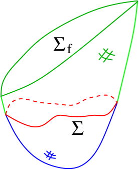
and our prescription is to integrate over all Euclidean/Lorentzian four-geometries $g$ of the form shown in Figure 1, with associated matter fields $\phi$, bounded by the three-geometry $\Sigma_{f}$ and matter fields present in the final state. The Euclidean region is essential because there is no way to ‘round off’ a Lorentzian manifold without introducing a boundary. We sum over all matching surfaces $\Sigma$ and Euclidean regions bounded by $\Sigma$. Our prescription differs from that of Hartle and Hawking [2] in that we shall not impose regularity of the four-geometries summed over. Such a prescription seems to us to be at odds with the basic principles of path integration. Regularity of the background geometry and the fluctuation modes should emerge as an output of the path integral rather than be input, and we shall see this occur in our calculations below.

The expression (1) is only formal, and part of our investigation will be to see whether we can calculate it in a perturbative expansion around saddle point solutions i.e. instantons. The relevant instantons are real solutions of the Euclidean field equations which possess a surface $\Sigma$ on which they may be analytically continued to a real Lorentzian spacetime. The condition for this to be possible is that the normal derivatives of the three-metric and matter fields should be zero on $\Sigma$. Note that regularity of the four-geometry of the instanton, needed here so that analytic continuation is possible, is a consequence of the instanton being a saddle point in the sum over all four-geometries and therefore a solution of a partial differential equation. Such analytic four-geometries are of course a set of measure zero in the original path integral.

FIG. 1.: The quantum amplitude for a three-geometry $\Sigma_{f}$ is given as the path integral over all Lorentzian geometries matched on a three-surface $\Sigma$ to a compact Euclidean four-manifold. All geometries of this type are to be integrated over.

We wish to calculate correlators of physical observables in the Lorentzian region. Each instanton provides a zeroth order approximation, giving us a classical background within which quantum fluctuations propagate. To first order in $\hbar$ the quantum fluctuations are specified by a Gaussian integral. One can perform the integral in the Euclidean region and then analytically continue in the coordinates of the background solution to find the quantum correlators in the Lorentzian region. As we shall now see, the analytic continuation is guaranteed to give real-valued Lorentzian fields and momenta if the background solution is real in both the Euclidean and Lorentzian regions.

The quantum mechanical amplitude for the fluctuations about a particular background solution $B$ is given from (1) by (henceforth we set $\hbar=1$)

$$\Psi_{B}[g^{3},\phi]\sim e^{iS_{B}(g_{B},\phi_{B})}\int^{\delta g^{3},\delta\phi}\left[{\cal D}\delta g\right]\left[{\cal D}\delta\phi\right]e^{i{\cal S}_{2}(\delta g,\delta\phi)}$$ (2)

where the metric $g=g_{B}+\delta g$ and fields $\phi=\phi_{B}+\delta\phi$. ${\cal S}_{2}$ is the action for second and higher order fluctuations. Let ${\cal P}(x_{1})$ and ${\cal Q}(x_{2})$ be two observables at $x_{1}$ and $x_{2}$ on $\Sigma_{f}$. Then their correlator is given by integrating $|\Psi|^{2}$ times ${\cal P}(x_{1}){\cal Q}(x_{2})$ over a complete set of observables ${\cal O}(x)$ on a final state three-surface $\Sigma_{f}$ containing $x_{1}$ and $x_{2}$,

$$\langle{\cal P}(x_{1}){\cal Q}(x_{2})\rangle={\cal N}\int dB\int\left[{\cal D}{\cal O}(\Sigma_{f})\right]\Psi_{B}\left[{\cal O}\right]^{*}\Psi_{B}\left[{\cal O}\right]{\cal P}(x_{1}){\cal Q}(x_{2})$$ (3)

with ${\cal N}$ an appropriate normalization constant. The full quantum correlator involves the sum over all background solutions $B$. If no other constraints are imposed, the solution with the lowest Euclidean action will dominate.

The insertion of the sum over a complete set of states means that the result (3) may be viewed a single ‘doubled’ path integral. The ‘initial’ state is established on the Euclidean region bounded by the first version of $\Sigma$. There is then a Lorentzian region running forward with weighting factor $e^{iS}$ to $\Sigma_{f}$ on which the operators of interest are located. Then there is a region running back to a second version of $\Sigma$, with weighting factor $e^{-iS}$, and finally the geometry closes on another Euclidean compact four-manifold. In the instanton approximation, the two Euclidean regions are actually copies of the same half-instanton. But the quantum fluctuations on the upper and lower halves are independent - the wavefunction $\Psi$ and its conjugate $\Psi^{*}$ involve independent integrations over the perturbations.

In formula (3) we can now continue $x_{1}$ and $x_{2}$ back into the Euclidean region of the background solution. If the Lorentzian continuation of the instanton is real, then as mentioned the Lorentzian part of the path integral involves a factor of $e^{iS}$ coming from $\Psi$ and a factor of $e^{-iS}$ from $\Psi^{*}$. These cancel exactly allowing us to deform $\Sigma_{f}$ back towards the Euclidean region. Upon reaching the Euclidean region however, we discover that both $\Psi$ and $\Psi^{*}$ involve $e^{-S_{E}}$ so there is no cancellation. In the correlator we are left with an overall $e^{-2S_{E}}$ where $S_{E}$ is the half-instanton action, and the action for the fluctuations is just the Euclidean action evaluated over the doubled half-instanton. Correlators calculated in the Euclidean region and continued to the Lorentzian region are therefore equal to those computed from the Lorentzian path integral with Euclidean no boundary initial conditions only if the background solution is real. Note that the cancellation of $e^{iS}$ and $e^{-iS}$ occurs for any three-surface $\Sigma_{f}$ in the Lorentzian region. There is no requirement that $\Sigma_{f}$ be spacelike. In fact, there is no reason for a complete surface $\Sigma_{f}$ to exist at all. If one computes correlators in the Euclidean region as we shall, all that matters is that a smooth continuation of local observables exists into the Lorentzian region. If there are singularities, they can be avoided by choosing an appropriate continuation contour.

The above construction is closely analogous to the imaginary time formalism for thermal field theory, where real-time correlators can be calculated by analytic continuation of Euclidean ones. In the present context, the compact nature of the Euclidean instantons has the same effect on correlators that the periodicity in imaginary time does in thermal field theory. The periodicity of the instanton solution introduces thermal weighting factors corresponding to the Hawking temperature of the background spacetime.

III Instantons and Analytic Continuation

Let us briefly recall the form of the instantons we are interested in. We consider Einstein gravity coupled to a single scalar field $\phi$ with potential energy $V(\phi)$. We seek finite-action solutions of the Euclidean equations of motion. If $V(\phi)$ has a positive extremum, there is a solution in the form of a four-sphere. This has the maximal symmetry allowed in four dimensions, namely $O(5)$. In general however, no such instanton exists, and the highest symmetry possible is $O(4)$. The instantons are described by the line element

$$ds^{2}=d\sigma^{2}+b^{2}(\sigma)d\Omega_{3}^{2}=d\sigma^{2}+b^{2}(\sigma)\left(d\psi^{2}+{\rm sin}^{2}(\psi)d\Omega_{2}^{2}\right)$$ (4)

with $b(\sigma)$ the radius of the three-sphere. The Einstein and scalar field equations take the form

$$\phi_{,\sigma\sigma}+3{b_{,\sigma}\over b}\phi_{,\sigma}=V_{,\phi},\qquad b_{,\sigma\sigma}=-{\kappa\over 3}b\left(\phi_{,\sigma}^{2}+V\right)$$ (5)

where $\kappa\equiv 8\pi G$, $\phi_{,\sigma}\equiv\partial_{\sigma}\phi$ and $V_{,\phi}\equiv\frac{dV}{d\phi}$.

The point of [3] was that for a gently sloping potential of the kind needed for inflation, there exists a one-parameter family of solutions to these equations labelled by the value of the scalar field at the north pole of the instanton. At the north pole the metric and scalar field are regular. At the south pole, which is singular, the scale factor goes to zero as $\left(\sigma_{m}-\sigma\right)^{\frac{1}{3}}$, and the scalar field diverges logarithmically in $\sigma$. These singular instantons are in general not stationary points of the action and they should be interpreted as constrained instantons, where the constraint is imposed on a small three-surface surrounding the singularity [8].

FIG. 2.: The Euclidean/Lorentzian manifold in the vicinity of the regular pole.

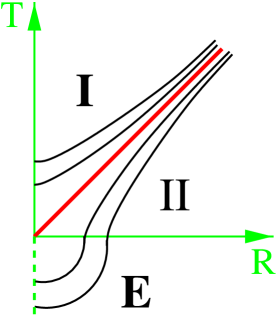
The various analytic continuations are fixed by the fact that the Euclidean/Lorentzian geometry in the neighbourhood of the north pole is locally flat. The coordinates we use for the instanton and its continuation reduce in this neighbourhood to those used in mapping flat space onto the Milne universe, see Figure 2. There is then an obvious choice of regular coordinates which allows one to uniquely fix the required continuations.

Consider flat Minkowski space with line element $-dT^{2}+dR^{2}+R^{2}d\Omega_{2}^{3}$. The analytic continuation to Euclidean time is performed by setting $T_{E}=iT$. Under this continuation the Lorentzian action $S$ yields the positive Euclidean action, $iS=-S_{E}$. We may describe the situation in O(4) invariant coordinates $T_{E}=\sigma\cos\Omega$, $R=\sigma\sin\Omega$, with $\Omega$ the polar angle on the three-sphere. These coordinates correspond to those used for our O(4) invariant instantons. As $\Omega$ runs from $\pi$ to zero, $T_{E}$ runs from $-\sigma$ to $\sigma$. For fixed $\sigma$, the Euclidean action involves the integral $\int_{-\sigma}^{\sigma}dT_{E}$. The continuation to the Lorentzian region is described by distorting the $T_{E}$ contour into the complex plane. The new contour runs from $-\sigma$ to zero, up the positive imaginary axis where the $e^{-S_{E}}$ factor gives $e^{iS}$ needed for the wavefunction $\Psi$ in (3). The continuation then runs back down the imaginary axis, giving $e^{-iS}$ and along the real axis from zero to $+\sigma$. If we translate $T_{E}$ into $\Omega$, the first two segments of the contour run from $\Omega=\pi$ to $\Omega=\pi/2$ and then down the line $\Omega=(\pi/2)-it^{\prime}$, with $t^{\prime}$ real and positive. The latter segment gives us the $e^{iS}$ term in the ‘doubled’ path integral.

Following this continuation on the surface $T_{E}=0$, from the Euclidean region we obtain a Lorentzian spacetime with timelike coordinate $t^{\prime}$. We have $T=\sigma\sinh t^{\prime}$ and $R=\sigma\cosh t^{\prime}$. Since these formulae imply $R^{2}-T^{2}>0$, these coordinates cover only part of the Lorentzian region, the exterior of the light cone emanating from the origin of spherical coordinates at $T=0$. We call this region II. We can then perform a second continuation $t^{\prime}=\chi-i{\pi\over 2}$ by setting $T=t\cosh\chi$ and $R=t\sinh\chi$ to obtain the metric in the interior of the light cone, which we call region I. In the vicinity of the regular pole, these new coordinates are those of the Milne universe. Globally, region I is the inflating open universe.

Hence the required continuations are

$${\rm Euclidean\rightarrow I:}\qquad\sigma=it,\qquad\Omega=-i\chi,$$ (6)

$${\rm Euclidean\rightarrow II:}\qquad\Omega={\pi\over 2}-it^{\prime},$$ (7)

yielding the following line elements

$${\rm Euclidean:}\qquad d\sigma^{2}+b^{2}(\sigma)d\Omega_{3}^{2},$$ (8)

$${\rm Region~{}I:}\qquad-dt^{2}+a^{2}(t)(d\chi^{2}+\sinh^{2}\chi d\Omega_{2}^{2}),$$ (9)

$${\rm Region~{}II:}\qquad d\sigma^{2}+b^{2}(\sigma)(-{dt^{\prime}}^{2}+\cosh^{2}t^{\prime}d\Omega_{2}^{2}).$$ (10)

The function $b(\sigma)\rightarrow\sigma$ as $\sigma\rightarrow 0$, and $a(t)\rightarrow t$ as $t\rightarrow 0$, so it follows from (7) that $b=ia$.

The Euclidean action is expressed as an integral over the coordinates $\sigma$ and $\Omega$, and then regarded as a four dimensional contour integral. We may then distort the integration contour into the regions of the complex coordinate space corresponding to the Lorentzian regions I and II. This procedure uniquely defines the path integral measure for Lorentzian correlators.

FIG. 3.: Contour for $X\left(t\right)$.

In what follows, it will be very useful to work in terms of a conformal spatial coordinate in the Euclidean region and in region II, defined by

$$X\equiv\int_{\sigma}^{\sigma_{m}}\frac{d\sigma^{\prime}}{b\left(\sigma^{\prime}\right)}.$$ (11)

For singular instantons, $X=0$ corresponds to the singular pole and $X\rightarrow\infty$ corresponds to the regular pole. For regular (Coleman-De Luccia) instantons, the second regular pole is at $X\rightarrow-\infty$.

It is also useful to work in a conformal time coordinate $\tau$ in the open universe, defined to obey $dt=a(t)d\tau$. For many purposes we shall need to relate $\tau$ to $X$. To do this we extend our integral definition of $X$ in equation (11) into the complex $\sigma$-plane. The required integration contour is shown in Figure 3. One has

$$X\equiv\int_{it}^{\sigma_{m}}\frac{1}{b\left(\sigma\right)}d\sigma=-\tau-i{\pi\over 2}$$ (12)

where we define the lower limit of the conformal time $\tau$ via

$$-\tau\equiv\lim_{\epsilon\rightarrow 0}\left(\int_{\epsilon}^{\sigma_{m}}\frac{d\sigma}{b\left(\sigma\right)}-\int_{\epsilon}^{t}\frac{dt^{\prime}}{a\left(t^{\prime}\right)}\right),$$ (13)

so that $\tau$ runs from $-\infty$ at the beginning of the open universe to an approximate constant when inflation is well underway, and then finally diverges logarithmically to $\infty$ at late times in the open universe when $a\left(t\right)\sim t$.

The conformal structure of the Lorentzian region is shown in Figure 4. As the diagram indicates, the singularity is timelike and visible from within the open universe region, labelled I. It is interesting to ask when the singularity first becomes visible to an observer in region I. Any such observer can by symmetry be placed at the origin of spherical coordinates. To find the null geodesics, we first change coordinates to conformal time in region I, defined in equation (13). Null geodesics incident on the origin of spherical coordinates, $\chi=0$, at a conformal time $\tau_{0}$ obey

$$\chi=\tau_{0}-\tau.$$ (14)

With the above continuations (7) the conformal space coordinate $X$ in region II obeys

$$X=t^{\prime}-\tau_{0}.$$ (15)

The singularity is located at $X=0$, and the transition from the Lorentzian to the Euclidean region is at $t^{\prime}=0$. It follows that singularity first becomes visible in the open universe when $\tau_{0}=0$. As mentioned above, with the above definition of $\tau$, inflation ends at negative conformal time. For example, for a ${1\over 2}m^{2}\phi^{2}$ potential with 60 efolds of inflation, we find the end of inflation occurs at $\tau=-1.70$ in units where the space curvature is minus one. Evolving forward into the late universe, one finds that the singularity is first visible at late times when universe is becoming curvature dominated.

FIG. 4.: Conformal spacetime structure of the classical background solution.

Although the singularity is visible within the open universe, and has a definite observable effect, as we shall see the quantum fluctuations are nevertheless well defined in its presence. The singularity acts as a reflecting boundary [15], and nothing enters the universe from it.

IV The Path Integral for Scalar Perturbations

In this section we derive the action appropriate for fluctuations about the instantons described above. Since the background solution satisfies the field equations (including an appropriate constraint if that is required [8]), the leading term in the action occurs at second order in the perturbations. We shall calculate this second order term and the perform the Gaussian path integral determining the quantum correlators to first order in $\hbar$.

We compute the relevant action in the open universe region, where a Hamiltonian treatment is straightforward. Our discussion follows the notation of ref. [13], although we shall work strictly from the path integral point of view. The action for scalar perturbations reduces to that for a single gauge-invariant variable $q$, related to the Newtonian potential $\Psi_{N}$ standardly used in the analysis of inflationary quantum fluctuations. We analytically continue the variable $q$ into the Euclidean region of the instanton, where its action is positive. The real-space correlator of $q$ is computed in the Euclidean region and finally analytically continued back into the Lorentzian region.

Following standard notation we write the perturbed line element and scalar field as

$$ds^{2} = a^{2}\left(\tau\right)\left(-\left(1+2A\right)d\tau^{2}+S_{i}dx^{i}d\tau+\left(\gamma_{ij}+h_{ij}\right)dx^{i}dx^{j}\right),$$ (16)

$$\phi = \phi_{0}\left(\tau\right)+\delta\phi$$ (17)

where $\gamma_{ij}$ is the metric on the background three-space, $\tau$ is the conformal time, $\phi_{0}\left(\tau\right)$ is the background acalar field and $a(\tau)$ is the background scale factor.

We decompose $S_{i}$ and $h_{ij}$ as follows (see [16])

$$h_{ij} = -2\psi\gamma_{ij}+2E_{|ij}+2F_{\left(i|j\right)}+t_{ij},$$ (18)

$$S_{i} = B_{|i}+V_{i}.$$ (19)

Here $|$ denotes covariant derivative on the background three-space, $\psi$, $B$ and $E$ are scalars, $V_{i}$ and $F_{i}$ are divergenceless vectors, and $t_{ij}$ is a transverse traceless tensor. In general, with a suitable asymptotic decay condition, the above decomposition is unique up to $B\rightarrow B+$constant, $F_{i}\rightarrow F_{i}+K_{i}$, with $K_{i}$ a Killing vector. For compact 3-spaces there is in addition an ambiguity since the metric is unchanged under $\psi\rightarrow\psi-\zeta$, $E\rightarrow E+\zeta$, with $\left(\Delta+3\right)\zeta=0$. However for the compact Euclidean instantons we consider all modes obeying $\left(\Delta+3\right)\zeta=0$ are actually pure gauge and we shall in any case have to project them out.

Under an infinitesimal scalar coordinate transformation $x^{\mu}\rightarrow x^{\mu}+\lambda^{\mu}$, where $\lambda^{\mu}=\left(\lambda^{0},\lambda^{|i}\right)$, the perturbations in (19) transform as

$$\psi\rightarrow\psi-{\cal H}\lambda^{0}, B\rightarrow B+\lambda^{\prime}-\lambda^{0},$$ (20)

$$A\rightarrow A+{\lambda^{0}}^{\prime}+{\cal H}\lambda^{0}, E\rightarrow E+\lambda,~{}~{}~{}~{}\delta\phi\rightarrow\delta\phi+\phi_{0}^{\prime}\lambda^{0}$$ (21)

where ${\cal H}\equiv a^{\prime}/a$, and here and below prime denotes derivative with respect to conformal time. The action is invariant under these transformations. We must pick a gauge in order to fix this invariance and obtain a unique result. As is well known, the computation of inflationary perturbations from a single scalar field is simplest in conformal Newtonian gauge, defined by setting $B=E=0$. This completely fixes the gauge freedom. Equivalently, one can define the gauge-invariant variable [1]

$$\Psi_{N}=\psi-{\cal H}\left(B-E^{\prime}\right).$$ (22)

As long as there are no anisotropic stresses, $\Psi_{N}$ is governed by a second order differential equation in time, and all perturbations are determined from $\Psi_{N}$ with the use of the Einstein constraint equations. An approximately-conserved quantity $\chi$ can be constructed from from $\Psi_{N}$ which may be used to match the super-Hubble radius perturbations across the reheating surface and into the late universe relevant for observation (see e.g. [4]).

In this section we derive the path integral appropriate for computing $\Psi_{N}$ correlators in the open universe. We shall do so in a manifestly gauge-invariant manner. The first point to note is that $\Psi_{N}$ involves a field velocity and in the path integral formalism the first step is to convert this to a canonical momentum. This requires us to use the Hamiltonian (first order) form of the path integral. A second merit of this formalism is that integration over the nondynamical lapse and shift fields imposes the Einstein constraint equations as delta functionals, enabling further integrations to be performed. Our discussion parallels that of Appendix B of reference [13], but is slightly more concise. We shall also be careful to keep certain surface terms which determine the allowed fluctuation modes about singular instantons.

Our starting point is the action for gravity plus a scalar field

$$S=\frac{1}{2\kappa}\int d^{4}x\sqrt{-g}\left(R-\frac{1}{2}\nabla_{\mu}\phi\nabla^{\mu}\phi-V\left(\phi\right)\right)-\frac{1}{\kappa}\int d^{3}x\sqrt{\gamma}K,$$ (23)

where $K$ is the trace of the extrinsic curvature of the boundary three-surface. The surface term is needed to remove second derivatives from the action, so that fluctuation variables are constrained on the boundary but their derivatives are not. The decomposition (19) is substituted into equation (23), keeping all terms to second order. The scalar, vector and tensor components decouple. The vector perturbations are uninteresting because the Einstein constraints force them to be zero. The tensor perturbations are discussed in the parallel paper [9]. The second order action for the scalar perturbations reads

$$S_{2} = \frac{1}{2\kappa}\int d\tau d^{3}xa^{2}\sqrt{\gamma}\bigg{\{}-6\psi^{\prime 2}-12{\cal H}A\psi^{\prime}+2\Delta\psi\left(2A-\psi\right)-2\left({\cal H}^{\prime}+2{\cal H}^{2}\right)A^{2}$$ (27)

$$+\kappa\left(\delta\phi^{\prime 2}+\delta\phi\Delta\delta\phi-a^{2}V_{,\phi\phi}\delta\phi^{2}\right)+2\kappa\left(3\phi_{0}^{\prime}\psi^{\prime}\delta\phi-\phi_{0}^{\prime}\delta\phi^{\prime}A-a^{2}V_{,\phi}A\delta\phi\right)$$

$$+{\cal K}\left(-6\psi^{2}+2A^{2}+12\psi A+2\left(B-E^{\prime}\right)\Delta\left(B-E^{\prime}\right)\right)$$

$$+4\Delta\left(B-E^{\prime}\right)(\frac{\kappa}{2}\phi_{0}^{\prime}\delta\phi-\psi^{\prime}-{\cal H}A)\bigg{\}}$$

where $\Delta$ is the Laplacian on the three-space. Integrations by parts in the spatial directions may be freely used in anticipation of the fact that the fluctuations are determined in the Euclidean region where the three-space is an $S^{3}$ so there are no surface terms. We shall eventually need to be more careful about integrating by parts with respect to $\tau$, at least in the case of singular instantons, because $\tau$ continues to the coordinate $X$ in the Euclidean region which terminates on the singular boundary. However, even here we may integrate by parts freely until we have expressed our action density in Hamiltonian form for the observable of interest, namely $\Psi_{N}$. After this last stage we need to be careful to retain all surface terms. As we shall see, after continuation to the Euclidean region these surface terms determine the set of allowed fluctuation modes.

We introduce the momenta canonically conjugate to $\psi$, $E$, and $\delta\phi$ as

$$\Pi_{\psi} = \frac{2a^{2}\sqrt{\gamma}}{\kappa}\left(-3\psi^{\prime}+3\frac{\kappa}{2}\phi_{0}^{\prime}\delta\phi-3{\cal H}A-\Delta\left(B-E^{\prime}\right)\right),$$ (28)

$$\Pi_{E} = \frac{2a^{2}\sqrt{\gamma}\Delta}{\kappa}\left(\psi^{\prime}-\frac{\kappa}{2}\phi_{0}^{\prime}\delta\phi+{\cal H}A-{\cal K}\left(B-E^{\prime}\right)\right),$$ (29)

$$\Pi_{\delta\phi} = a^{2}\sqrt{\gamma}\left(\delta\phi^{\prime}-\phi_{0}^{\prime}A\right).$$ (30)

We shall only consider modes for which $-\Delta-3{\cal K}$ is positive, and in this case $\Pi_{\psi}$ and $\Pi_{E}$ are independent and we can solve for the velocities in terms of fields and momenta. As an aside, we mention a subtlety associated with the modes known in the literature as ‘bubble wall’ fluctuation modes [17], [18]. These modes have have $\Delta+3{\cal K}=0$. Such perturbation modes are possible in the open universe in spite of the fact that they possess the ‘wrong sign’ for the Laplacian and therefore grow exponentially with comoving radius. However, if one expands in harmonics, for $l<2$ such modes may be gauged away. And modes with $l\geq 2$ are singular when continued into the Euclidean region, since with $\Delta_{E}\equiv-\left(n^{2}-1\right)=-3$ the regular eigenfunctions all have $l<n=2$. So there are no physical fluctuation modes with $\Delta+3{\cal K}=0$. However, our gauge-invariant action will be zero for the $\Delta+3{\cal K}=0$ gauge modes, and we will need to project out their contribution at various stages of the calculation.

Proceeding with this caveat, we rewrite the action (27) in first order form

$$S_{2} = \int d\tau d^{3}x\Bigg{\{}\Pi_{\psi}\psi^{\prime}+\Pi_{E}E^{\prime}+\Pi_{\delta\phi}\delta\phi^{\prime}$$ (34)

$$-\frac{\kappa}{4a^{2}\sqrt{\gamma}\left(\Delta+3{\cal K}\right)}\left(-{\cal K}\Pi_{\psi}^{2}+2\Pi_{\psi}\Pi_{E}+\frac{3}{\Delta}\Pi_{E}^{2}+\frac{2\left(\Delta+3{\cal K}\right)}{\kappa}\Pi_{\delta\phi}^{2}\right)-\frac{\kappa}{2}\phi_{0}^{\prime}\Pi_{\psi}\delta\phi$$

$$-\frac{a^{2}\sqrt{\gamma}}{\kappa}\left(\left(\Delta+3{\cal K}\right)\psi^{2}-\frac{\kappa}{2}\left(\Delta+3{\cal K}-{\cal H}^{2}-{\cal H}^{\prime}+\frac{\phi^{\prime\prime\prime}_{0}}{\phi_{0}^{\prime}}\right)\delta\phi^{2}\right)$$

$$-B\Pi_{E}-A\left(-{\cal H}\Pi_{\psi}+\phi^{\prime}_{0}\Pi_{\delta\phi}+\frac{2a^{2}\sqrt{\gamma}}{\kappa}\left(-\left(\Delta+3{\cal K}\right)\psi+\frac{\kappa}{2}\left({\cal H}\phi_{0}^{\prime}-\phi^{\prime\prime}_{0}\right)\delta\phi\right)\right)\Bigg{\}}.$$

As stated above, we would like to evaluate the correlator for the gauge-invariant variable $\Psi_{N}$. We may express $\Psi_{N}$ as a dynamical variable in terms of fields and momenta as follows

$$\Psi_{N}=\psi+\frac{{\cal H}\kappa}{2a^{2}\sqrt{\gamma}}\left(\frac{\Delta\Pi_{\psi}+3\Pi_{E}}{\Delta\left(\Delta+3{\cal K}\right)}\right).$$ (35)

This is singular for $\Delta=0$ so our discussion will only be valid for the inhomogeneous perturbations, which is all we shall calculate here. The homogeneous perturbation modes require a separate treatment because the Euclidean action is not positive and to cure this the conformal factor must be decoupled from the physical degrees of freedom. We do not address this problem here, but shall simply project out the homogeneous modes on the $S^{3}$ or $H^{3}$ at each stage of the calculation.

We now add a source term $-i\int J_{N}\Psi_{N}$ to the quadratic action, and perform the path integral over all fields and momenta. The non-dynamical variables A and B only occur linearly in $S_{2}$, and functional integration over these fields gives us delta functionals imposing the $G_{0i}$ and $G_{00}$ Einstein constraints. We use these delta functionals to perform the $\Pi_{E}$ and $\Pi_{\delta\phi}$ integrals. This sets $\Pi_{E}$ to zero in the term multiplying the source. There is then no residual $E$ dependence in the action and and the functional integral over $E$ is ignored as an infinite gauge orbit volume.

There is still a residual gauge freedom in the action, corresponding to $\lambda^{0}$ reparametrizations (see above). However the action density can be expressed, up to a total derivative, in terms of $\Psi_{N}$ and its canonically conjugate gauge-invariant variable

$$\Pi_{N} = {1\over 2}\Pi_{\psi}-{a^{2}\sqrt{\gamma}\over\kappa{\cal H}}\left(\Delta+3{\cal K}\right)\psi-{2a^{2}\sqrt{\gamma}\over\kappa\phi_{0}^{\prime}}\left(\Delta+3{\cal K}\right)\delta\phi.$$ (36)

The action density is now independent of $\delta\phi$, so this too can be integrated out as a gauge orbit volume.

It is convenient to rescale the coordinate $q={2a\over\kappa\phi_{0}^{\prime}}\Psi_{N}$, the momentum $p={\kappa\phi_{0}^{\prime}\over 2a}\Pi_{N}$, and the source $J_{q}=\frac{\kappa\phi^{\prime}}{2a}J_{N}$. We then perform an integration by parts to represent the action in canonical form $S=\int\left[pq^{\prime}-H(p,q)\right]$. From now on, all surface terms must be kept. Finally, we perform the Gaussian integral over the momentum variable $p$ to obtain the reduced action for $q$,

$$iS_{2}\left(J\right) = -{i\over 2}\int d\tau d^{3}x\sqrt{\gamma}\Bigg{\{}\left(\Delta+3{\cal K}\right)q\left(\hat{O}+\Delta+3{\cal K}\right)q$$ (37)

$$+ \left(\Delta+3{\cal K}\right)\left[qq^{\prime}+\left(\frac{\kappa\phi^{\prime 2}_{0}}{4{\cal H}}+\frac{\phi^{\prime\prime}_{0}}{\phi^{\prime}_{0}}\right)q^{2}\right]^{\prime}\Bigg{\}}+\int J_{q}q$$ (38)

where

$$\hat{O}\equiv-\frac{d^{2}}{d\tau^{2}}+\frac{\kappa}{2}(\phi_{0}^{\prime})^{2}+\phi_{0}^{\prime}\left(\frac{1}{\phi_{0}^{\prime}}\right)^{\prime\prime}.$$ (39)

The result for the bulk term agrees, up to a sign, with that obtained in [13]. We are now ready to analytically continue to the Euclidean region and perform the Gaussian integral to obtain the $qq$ correlator.

V The Euclidean Green Function

The continuation to the Euclidean region is performed as described above, in equation (7). The Laplacian $\Delta$ continues to $-\Delta_{3}$, where $\Delta_{3}$ is the Laplacian on $S^{3}$ and the constant ${\cal K}$ continues to itself. We set ${\cal K}=-1$ from now on. Finally, the variable $q$ continues to itself.

The Euclidean action is given by

$$iS_{2}\left(J\right) = -S_{2}^{E}\left(J\right)=-{1\over 2}\int dXd^{3}\Omega_{3}\Bigg{\{}\left(-\Delta_{3}-3\right)q\left(\hat{O}-\Delta_{3}-3\right)q$$ (40)

$$+ \left(-\Delta_{3}-3\right)\left[qq^{\prime}+\left(\frac{\kappa\phi^{\prime 2}_{0}}{4{\cal H}}+\frac{\phi^{\prime\prime}_{0}}{\phi^{\prime}_{0}}\right)q^{2}\right]^{\prime}\Bigg{\}}+\int J_{q}q$$ (41)

where the volume element on the three-sphere is $d^{3}\Omega_{3}$ and now

$$\hat{O}\equiv-\frac{d^{2}}{dX^{2}}+\frac{\kappa}{2}(\phi_{0}^{\prime})^{2}+\phi_{0}^{\prime}\left(\frac{1}{\phi_{0}^{\prime}}\right)^{\prime\prime}\equiv-\frac{d^{2}}{dX^{2}}+U(X).$$ (42)

where primes now denote derivatives with respect to $X$. The bulk term in the action is positive definite for the inhomogeneous modes of interest, as was noted by Lavrelashvili [19].

The path integral over $q$ is Gaussian and is performed by solving the classical field equation for $q(J)$ and substituting back. After the appropriate normalization, we obtain the generating functional for $q$ correlators, exp$({1\over 2}\int\int JG_{E}J)$, where $G_{E}$ is the Euclidean Green function. The two point correlator is then $\langle q\left({\bf X}\right)q\left({\bf X^{\prime}}\right)\rangle=G_{E}({\bf X},{\bf X^{\prime}})$. The Euclidean Green function is the solution to the equation

$$\left(-\Delta_{3}-3\right)\left(\hat{O}-\Delta_{3}-3\right)G_{E}=g^{-{1\over 2}}\delta^{(4)}({\bf X}-{\bf X^{\prime}})-\delta(X-X^{\prime})\frac{\sin 2\Omega}{\pi^{2}\sin\Omega}.$$ (43)

Here ${\bf X}=(X,x^{i})$, and $g$ is the determinant of the metric. $\Omega$ is the angle between the two points $x$ and $x^{\prime}$ on the three-sphere. The second term on the right hand side of equation (43) is present because we project out the $-\Delta_{3}=3$ gauge modes as mentioned above. Its coefficient is fixed by the requirement that the right hand side be orthogonal to the $-\Delta_{3}=3$ modes under integration over the three-sphere. We shall also project out the $\Delta=0$ homogeneous mode, but for the sake of brevity we shall not write out the relevant terms explicitly.

Equation (43) is solved by expressing both $\delta(X-X^{\prime})$ and $G_{E}$ as sums over a complete set of eigenmodes of $\hat{O}$ and equating coefficients. $\hat{O}$ is a Schrödinger operator, and its eigenfunctions obey

$$\hat{O}\psi_{p}(X)=\left(-{d^{2}\over dX^{2}}+U(X)\right)\psi_{p}(X)=(p^{2}+4)\psi_{p}(X),$$ (44)

where the potential $U(X)$ is given in equation (42). Near the regular pole of the instanton i.e. $X\rightarrow\infty$, we have $\phi_{0,\sigma}\sim\sigma\sim e^{-X}$, so that $\phi_{0}^{\prime}\sim e^{-2X}$, and $U\rightarrow 4$. There is therefore a positive continuum starting at $p^{2}=0$. For gently sloping inflationary potentials, there is also generally a single bound state with $-1<p^{2}<0$.

For singular instantons, near $X=0$ the potential term is repulsive and diverges as $\frac{3}{4X^{2}}$, as noted by Garriga [15]. There are two sets of eigenmodes of $\hat{O}$ for each $p$, behaving as $X^{-1/2}$ or as $X^{3/2}$ for small $X$ respectively. Now the importance of keeping the surface terms in the Euclidean action (41) becomes clear. The surface terms are positive infinity for the divergent modes. Thus the Euclidean action by itself completely determines the allowed spectrum of fluctuations. Regularity of the eigenmodes does not need to be imposed as an additional, external condition. Only fluctuations vanishing at the singularity are allowed, so in effect the singularity enforces Dirichlet boundary conditions.

Now consider for fixed real $p$ the solution to the Schrödinger equation (44) which behaves as $X^{\frac{3}{2}}$ for $X\rightarrow 0$, which we shall denote $\psi_{p}(X)$. Being the solution to a differential equation with finite coefficients, this is analytic for all finite $p$ in the complex $p$-plane [20]. It is also useful to define the Jost function $g_{p}(X)$ as the solution which tends to $e^{ipX}$ as $X\rightarrow\infty$. This is analytic in the upper half complex $p$-plane, as seen by iterating the integral equation [21]

$$g_{p}(X)=e^{ipX}+\frac{1}{p}\int_{X}^{\infty}\sin p(Y-X)\,V(Y)\,g_{p}(Y)\,dY.$$ (45)

The two solutions are related via

$$\psi_{p}(X)=a_{p}g_{p}(X)+b_{p}g_{-p}(X).$$ (46)

Since the differential equation is even in $p$, $\psi_{-p}(X)=\psi_{p}(X)$ and $b_{p}=a_{-p}$. Completeness of the eigenfunctions then allows us to write the following representation of the delta function,

$$\delta\left(X-X^{\prime}\right)=\int_{-\infty}^{\infty}\frac{\psi_{p}\left(X\right)\psi_{p}\left(X^{\prime}\right)}{4\pi a_{p}a_{-p}}dp+\psi^{N}_{i\Lambda}\left(X\right)\psi^{N}_{i\Lambda}\left(X^{\prime}\right),$$ (47)

where we have included the contribution of a single assumed normalized bound state wavefunction $\psi_{i\Lambda}^{N}(X)$. One may check the normalization of the continuum contribution in equation (47) as follows. For $X$ and $X^{\prime}$ large, substituting in (46) one sees that the terms going as $e^{\pm ip(X-X^{\prime})}$ integrate to give the correctly normalized delta function.

It is also instructive to see how the right hand side vanishes for any $X\neq X^{\prime}$. For definiteness let us take $X>X^{\prime}$. Substituting the decomposition (46) into the integral for $\psi_{p}(X)$, we have

$$\int_{-\infty}^{\infty}\frac{\psi_{p}\left(X\right)\psi_{p}\left(X^{\prime}\right)}{4\pi a_{p}a_{-p}}dp = \int_{-\infty}^{\infty}\frac{\left(a_{p}g_{p}(X)+a_{-p}g_{-p}(X)\right)\psi_{p}\left(X^{\prime}\right)}{4\pi a_{p}a_{-p}}dp$$ (48)

$$= \int_{-\infty}^{\infty}\frac{g_{p}\left(X\right)\psi_{p}\left(X^{\prime}\right)}{2\pi a_{-p}}dp.$$ (49)

We now distort the integral onto a semicircle at infinity in the upper half $p$-plane. The contour at infinity gives no contribution since $g_{p}(X)\psi_{p}(X^{\prime})$ decays exponentially, as $e^{ip(X\pm X^{\prime})}$. Since $\psi_{p}(X^{\prime})$ is analytic for all $p$, and $g_{p}(X)$ is analytic in the upper half $p$-plane, the only contribution to the integral comes from zeroes of $a_{-p}$ in the upper half $p$-plane. These zeroes correspond to bound states as may be seen from the expression (46). If $a_{-p}$ vanishes, the corresponding solution decays exponentially at large $X$. Thus for each zero of $a_{-p}$ we have a normalizable bound state with eigenvalue $p^{2}$. But the Schrödinger equation only has real eigenvalues, so this is only possible for imaginary $p=i\Lambda$, with $\Lambda$ real.

Next we compute the residue of the pole, which we assume to be simple. From the Schrödinger equation one obtains the following identity

$$\left(\psi\frac{\partial\psi^{\prime}}{\partial p}-\frac{\partial\psi}{\partial p}\psi^{\prime}\right)^{\prime}=-2p\psi^{2}.$$ (50)

We integrate both sides over $X$ from zero to infinity. The left hand side yields a difference of surface terms. Only the surface term at infinity is non-zero, and we evaluate it using the asympotic form for $\psi_{p}$. Near $p=i\Lambda$, $a_{-p}$ vanishes as $\left(p-i\Lambda\right).\partial_{p}a_{-p}|_{p=i\Lambda}$. Then the integrated equation (50) gives us $\partial_{p}a_{-p}|_{p=i\Lambda}=-\frac{i\mathcal{N}}{a_{i\Lambda}}$, where the normalization constant ${\cal N}\equiv\int_{0}^{\infty}\psi_{i\Lambda}^{2}dX$. So the contribution from the zero of $a_{-p}$ to the integral (49) is just $\frac{-a_{i\Lambda}^{2}}{\mathcal{N}}g_{i\Lambda}(X)g_{i\Lambda}(X^{\prime})$. But $\frac{a_{i\Lambda}}{\sqrt{\mathcal{N}}}g_{i\Lambda}(X)$ is precisely the normalized bound state wavefunction $\psi^{N}_{i\Lambda}(X)$, so the contribution from the zero of $a_{-p}$ is exactly cancelled by the bound state term in (47). Hence the right hand side is zero as required.

All of this is simply understood. Imagine deforming our potential $U(X)$ to one possessing no bound state. Then the integral in (49), with $p$ running along the real axis, would give the delta function with no bound state contribution being needed. Now as one deforms the potential back to $U(X)$, a zero in $a_{-p}$ corresponding a bound state would appear first at $p=0$. This yields a pole in the integrand of (49) but the contour may be deformed above it since the rest of the integrand is analytic in the upper half $p$-plane. As the potential becomes more and more negative, the zero of $a_{-p}$ moves up the imaginary $p$ axis to $p=i\Lambda$. But the integral still equals $\delta(X-X^{\prime})$ as long as one takes the contour above the pole (see Figure 5). If one deforms the contour back to the real $p$ axis, the bound state contribution discussed above is produced from the residue of the pole.

FIG. 5.: Contour of integration avoiding the bound state pole.

In the case of non-singular instantons, a similar procedure may be followed. Here, since $b(\sigma)$ goes linearly to zero at each pole, $X$ should be defined as $\int_{\sigma}^{\sigma_{t}}\frac{d\sigma^{\prime}}{b\left(\sigma^{\prime}\right)}$, where $\sigma_{t}$ is say the value of $\sigma$ for which $b(\sigma)$ is a maximum. Then $X$ ranges from $-\infty$ to $\infty$, and for each value of $p^{2}$ we need two linearly independent mode functions. These may be taken to be $g_{p}^{\mathrm{left}}\left(X\right)$, defined to tend to $e^{-ipX}$ as $X\rightarrow-\infty$, and $g_{p}^{\mathrm{right}}\left(X\right)$, defined to tend to $e^{ipX}$ as $X\rightarrow\infty$. These can be shown to be orthogonal, and analytic in the upper half $p$-plane. As $X\rightarrow\infty$, if we write $g_{p}^{\mathrm{left}}\left(X\right)\rightarrow c_{p}e^{ipX}+d_{p}e^{-ipX}$, then as $X\rightarrow-\infty$, $g_{p}^{\mathrm{right}}\left(X\right)\rightarrow d_{p}e^{ipX}-c_{-p}e^{-ipX}$. Finally, we may express $\delta\left(X-X^{\prime}\right)$ as $\int_{-\infty}^{\infty}\frac{g_{p}^{\mathrm{right}}\left(X\right)g_{p}^{\mathrm{left}}\left(X^{\prime}\right)}{2\pi d_{p}}dp+\psi^{N}_{i\Lambda}\left(X\right)\psi^{N}_{i\Lambda}\left(X^{\prime}\right)$ in close analogy with the singular case.

Returning to our discussion of the singular case, from the representation (47) of the delta function we may now construct the following ansatz for the Green function

$$G_{E}=\int_{-\infty}^{\infty}C_{p}\left(\Omega\right)\frac{\psi_{p}\left(X\right)\psi_{p}\left(X^{\prime}\right)}{4\pi a_{p}a_{-p}}dp+C_{i\Lambda}\left(\Omega\right)\psi^{N}_{i\Lambda}\left(X\right)\psi^{N}_{i\Lambda}\left(X^{\prime}\right)$$ (51)

where as above $\Omega$ is the angle between the two points $x^{i}$ and ${x^{i}}^{\prime}$ on the three-sphere.

Substituting (51) into (43) we obtain an equation governing the ‘universal’ part of the correlator, $C_{p}\left(\Omega\right)$. This reads

$$(\tilde{\Delta}+3)(\tilde{\Delta}-1-p^{2})C_{p}\left(\Omega\right)=\delta^{3}(\Omega)-\frac{\sin 2\Omega}{\pi^{2}\sin\Omega},$$ (52)

where $\tilde{\Delta}\equiv\partial_{\Omega}^{2}+2\cot\Omega\partial_{\Omega}$.

We first find the particular integral for the term on the far right and then the four linearly independent solutions of the homogeneous equation. The latter are

$$\frac{\cos 2\Omega}{\sin\Omega},\frac{\sin 2\Omega}{\sin\Omega},\frac{\cosh p\Omega}{\sin\Omega},\mbox{~{}and~{}}\frac{\sinh p\Omega}{\sin\Omega}.$$ (53)

We combine the 2 solutions singular at $\Omega=0$ to cancel their leading singularities, and arrange that the term linear in $\Omega$ at small $\Omega$ has the correct coefficient to match the delta function in (52). Then we choose the coefficient of $\sinh p\Omega/\sin\Omega$ to make $C_{p}$ finite at $\Omega=\pi$ (i.e. for antipodal points on the $S^{3}$). Finally we choose the coefficient of the $\sin 2\Omega/\sin\Omega$ term to make the projection of $C_{p}$ onto the gauge modes zero. Hence we find

$$C_{p}\left(\Omega\right)=\frac{1}{4\pi\left(p^{2}+4\right)}\frac{\sinh p\left(\Omega-\pi\right)}{\sinh p\pi\sin\Omega}+\frac{\left(\pi-\Omega\right)\cos 2\Omega}{4\pi^{2}\left(p^{2}+4\right)\sin\Omega}+$$ (54)

$$\left(\frac{1}{\pi^{2}\left(p^{2}+4\right)^{2}}-\frac{1}{16\pi^{2}\left(p^{2}+4\right)}\right)\frac{\sin 2\Omega}{\sin\Omega},$$ (55)

where the first term gives us the contribution one might expect by analogy with the usual Euclidean scalar field vacuum. We shall be interested in the behaviour of $C_{p}\left(\Omega\right)$ in the complex $p$-plane. Here, the role of the extra terms is just to remove the double pole at $p=2i$. Had we written out the terms involving the homogeneous mode on the three-sphere, we would find that their effect would be to remove the pole at $p=i$.

We now have a convergent expression for $G_{E}$ in the Euclidean region. Note that whilst $G_{E}$ is perhaps most naturally expressed as a sum of regular eigenmodes, discrete because the space is compact, we have instead expressed it as an integral. The integral formula is more useful for analytic continuation since it is already close to an expression of the form we desire in the open universe, namely a integral over a continuum of modes.

Nevertheless it is interesting to see how the Euclidean Green function appears as a discrete sum. For $X>X^{\prime}$, we may close the $p$ contour above to obtain an infinite sum, convergent in the Euclidean region,

$$\sum^{\infty}_{n=3}\frac{1}{4\pi^{2}\left(n^{2}-4\right)}\frac{\sin n\Omega}{\sin\Omega}{g_{ni}(X)\psi_{ni}(X^{\prime})\over a_{-ni}},$$ (56)

where $g_{ni}(X)\sim e^{-nX}$ at large $X$. This demonstrates that our Green function is analytic in proper distance $\sigma\sim e^{-X}$ at the north pole of the instanton, as it should be. For non-singular instantons the argument generalizes to show that the Green function is analytic at the south pole too.

VI The Lorentzian Green Function

We now wish to continue our integral formula for the Green function given by (51), (55) into the open universe region. This involves setting $\Omega=-i\chi$ and continuing the conformal coordinate as described in equation (12).

To perform the continuation we take $X>X^{\prime}$ and write $G_{E}$ as

$$\int_{\cal C}\frac{g_{p}(X)\psi_{p}(X^{\prime})}{2\pi a_{-p}}C_{p}(\Omega)dp$$ (57)

where the contour ${\cal C}$ for the $p$ integral has been deformed above the bound state pole as described above (see Figure 5).

We can perform the analytic continuation $\Omega=-i\chi$ immediately. However, the $X$ continuation is more subtle, because $g_{p}\sim e^{ipX}$ at large $X$, and unless we are careful terms like $\sim e^{p\pi}$ occur which cause the $p$ integral to diverge. We circumvent this problem as follows. For $X-X^{\prime}>0$ we have

$$\int_{C}dp\frac{g_{p}(X)\psi_{p}(X^{\prime})}{2\pi a_{-p}}{e^{ip\chi}\over\left(p^{2}+4\right)}={e^{-2\chi}\over 16\pi^{2}}\frac{g_{2i}(X)\psi_{2i}(X^{\prime})}{a_{-2i}}$$ (58)

since the integrand is analytic in the upper half $p$-plane and the integral may be closed above. By inserting ${\sinh}p\pi/{\sinh}p\pi=1$ under the integral one sees that the integral (58) with a factor $e^{p\pi}/{\sinh}p\pi$ inserted is equal to that with a factor $e^{-p\pi}/{\sinh}p\pi$ inserted, plus the remaining term on the right hand side. We use this identity to re-express the term from (55) behaving as $e^{p\pi+i\chi}$.

The term on the right hand side of (58) may be then combined with the analytic continuation of the term involving $\pi\cos 2\Omega$ on the right hand side of (55) to produce a term proportional to $\sinh 2\chi/\sinh\chi$. The remaining terms in the correlator arising from the second and third terms in (55) are proportional to $\chi\cosh 2\chi/\sinh\chi$ and $\sinh 2\chi/\sinh\chi$. These, and the constant terms we have not written explicitly, are zero modes of the operators $\Delta$, $\Delta+3{\cal K}$ or $(\Delta+3{\cal K})^{2}$ and are therefore homogeneous modes or gauge modes which should be ignored.

After these simplifications, we rewrite our partially-continued correlator as

$$\int_{\cal C}{dp\over 8\pi^{2}(p^{2}+4)}{{\sin}p\chi\over{\sinh}\chi}{e^{-p\pi}\over{\sinh}p\pi}{g_{p}(X)\over a_{-p}}\psi_{p}(X^{\prime})$$ (59)

and insert the expression (46) to obtain

$$\int_{\cal C}{dp\over 8\pi^{2}(p^{2}+4)}{{\sin}p\chi\over{\sinh}\chi}{e^{-p\pi}\over{\sinh}p\pi}\left[g_{p}(X)g_{-p}(X^{\prime})+{a_{p}\over a_{-p}}g_{p}(X)g_{p}(X^{\prime})\right].$$ (60)

We are now ready to perform the analytic continuation $X=-i{\pi\over 2}-\tau$ under the integral. Under this substitution, we have

$$g_{\pm p}(X)\rightarrow e^{\pm p\pi\over 2}g^{L}_{\pm p}(\tau)$$ (61)

where the Lorentzian Jost function $g_{p}^{L}(\tau)$ is defined to be solution to the Lorentzian perturbation equation $\hat{O}g_{p}^{L}(\tau)=(p^{2}+4)g_{p}^{L}(\tau)$ obeying $g_{p}^{L}(\tau)\rightarrow e^{-ip\tau}$ as $\tau\rightarrow-\infty$. Equation (61) follows by matching at large $X$. Like $g_{p}(X)$, the Lorentzian Jost function $g_{p}^{L}(\tau)$ is analytic in the upper half $p$-plane.

The correlator now reads

$$\int_{\cal C}{dp\over 8\pi^{2}(p^{2}+4)}{{\sin}p\chi\over{\sinh}\chi}{1\over{\sinh}p\pi}\left[e^{-p\pi}g_{p}^{L}(\tau)g_{-p}^{L}(\tau^{\prime})+{a_{p}\over a_{-p}}g_{p}^{L}(\tau)g_{p}^{L}(\tau^{\prime})\right].$$ (62)

We want to distort the contour of integration ${\cal C}$ back to the real $p$ axis. This is only possible provided $g_{-p}$ is analytic in the region through which the contour is moved.

Analyticity of $g_{-p}$ in the strip $0<\Im(p)<1$ is proven as follows. One may re-express the Lorentzian perturbation equation $\hat{O}q=(p^{2}+4)q$ in terms of Lorentzian proper time $t$. The equation then takes the form $t^{2}\ddot{q}+A(t)t\dot{q}+B(t)q=-p^{2}q$. The coefficients $A(t)$ and $B(t)$ have Taylor expansions in $t$ about $t=0$. One now seeks power series solutions $q\sim t^{s}(1+q_{1}t+q_{2}t^{2}+...)$ and finds the appropriate indicial equation for $s$ and recursion relation for the coefficients. Here we obtain $s=\pm ip$, and a recursion relation that is non-singular as long as $p$ is not an integer times $i$. In this situation, one is guaranteed that the series for $q(t)$ converges within a circle extending to the nearest singularity of the differential equation [22], and even then the solution may be defined by analytic continuation around that singularity. In our case the first singularity occurs on the real axis when the background scalar field velocity $\dot{\phi}_{0}$ is zero, when inflation is over and reheating has begun. Matching across that singularity is accomplished by switching from $q$ to $\Psi_{N}$, and will not present any difficulties.

Since $g_{-p}$ is analytic in the desired region, we may now distort the countour ${\cal C}$ back to the real $p$ axis, recovering the bound state term from the simple pole at $p=i\Lambda$. Once the integral is along the real axis we use symmetry under $p\rightarrow-p$ to rewrite it as

$$\int_{-\infty}^{\infty} {dp\over 16\pi^{2}(p^{2}+4)}{{\sin}p\chi\over{\sinh}\chi}\Bigg{(}{\rm coth}p\pi\left[g_{p}^{L}(\tau)g_{-p}^{L}(\tau^{\prime})+g_{-p}^{L}(\tau)g_{p}^{L}(\tau^{\prime})\right]$$ (63)

$$- \left[g_{p}^{L}(\tau)g_{-p}^{L}(\tau^{\prime})-g_{-p}^{L}(\tau)g_{p}^{L}(\tau^{\prime})\right]+{1\over{\sinh}p\pi}\left[{a_{p}\over a_{-p}}g_{p}^{L}(\tau)g_{p}^{L}(\tau^{\prime})+{a_{-p}\over a_{p}}g_{-p}^{L}(\tau)g_{-p}^{L}(\tau^{\prime})\right]\Bigg{)}.$$ (64)

Note that for real $p$, $g^{L}_{-p}(\tau)$ is the complex conjugate of $g_{p}^{L}(\tau^{\prime})$ and $a_{-p}$ is the complex conjugate of $a_{p}$, so the second term in square brackets is imaginary, but the first and third terms are real.

We have the correlator in the Lorentzian region. Recall that the derivation assumed $X-X^{\prime}>0$. This translates to $\tau^{\prime}>\tau$, and we have calculated the Feynman (time ordered) correlator for all $\chi$ subject to this condition. For cosmological applications we are usually interested in the expectation value of some quantity squared, like the microwave background multipole moments or the Fourier modes of the density field. For this purpose, all that matters is the symmetrized correlator $\langle\{q(\chi,\tau),q(0,\tau^{\prime})\}\rangle$ which is just the real part of the Feynman correlator. The symmetrised correlator also represents the ‘classical’ part of the two point function and in the situations of interest it will be much larger than the imaginary piece.

The second term in (64) is pure imaginary and does not contribute to the symmetrized correlator. The other terms combine to give our final result

$$\langle\{\Psi_{N}(\chi,\tau),\Psi_{N}(0,\tau^{\prime})\}\rangle ={4\over\kappa^{2}\dot{\phi_{0}}(\tau)\dot{\phi_{0}}(\tau^{\prime})}\times$$ (65)

$$\Bigg{[}\int_{0}^{\infty}\frac{dp}{4\pi^{2}\left(p^{2}+4\right)} \frac{\sin p\chi}{\sinh\chi}\Re\left(\coth p\pi g_{p}^{L}(\tau)g_{-p}^{L}(\tau^{\prime})+\frac{1}{\sinh p\pi}\left(\frac{a_{p}}{a_{-p}}g_{p}^{L}\left(\tau\right)g_{p}^{L}(\tau^{\prime})\right)\right)$$ (67)

$$+\frac{1}{4\pi\left(4-\Lambda^{2}\right)}\frac{\sinh\Lambda\chi}{\sinh\chi}\frac{a_{i\Lambda}^{2}}{\mathcal{N}}\frac{g^{L}_{i\Lambda}\left(\tau\right)g^{L}_{i\Lambda}\left(\tau^{\prime}\right)}{\sin\Lambda\pi}\Bigg{]}$$

where the bound state pole arises as mentioned above from distorting the contour across the pole at $p=i\Lambda$ and we have converted the final integral along the real axis to one from $0$ to $\infty$. We have also converted from $q$ variable to $\Psi_{N}$ by multiplying by the appropriate factor where dots denote derivatives with respect to Lorentzian proper time. Also recall that units here are such that the comoving curvature scale is unity (${\cal K}=-1$).

The first term in this formula is essentially identical to that derived by [4] and [10], although in those derivations it was obtained only as an approximation. The second term, representing the reflection amplitude for waves incident from the regular pole, is only important at low $p$, since the $\sinh p\pi$ denominator suppresses it exponentially at high $p$. Finally, the bound state term produces long range correlations beyond the curvature scale. For large $p$ we recover the usual scale-invariant spectrum of inflationary quantum fluctuations. To see this note that at large $p$, $|g_{p}^{L}\left(\tau\right)|\rightarrow 1$. Then according to (67) there are equal contributions to the variance $\langle\Psi_{N}^{2}(0,\tau)\rangle$ from each logarithmic interval in $p$ at large $p$.

As mentioned in the introduction, one of our main concerns is to establish the differences between perturbations about singular and non-singular instantons. The above derivation was for singular instantons. It is straightforward to follow the argument through for non-singular instantons, where the coordinate $X$ now runs from $-\infty$ instead of zero. The only change in the final formula (67) is that the phase factor $a_{p}/a_{-p}$ is replaced by $c_{p}/d_{p}$, which is the reflection amplitude for waves incident on the potential from $X=+\infty$.

VII Conclusions

We have derived a general formula (67) for the time dependent correlator of the Newtonian potential in open inflationary universes resulting from Euclidean cosmological instantons. The phase shifts and mode normalizations in the Euclidean region can be calculated numerically, and the Lorentzian Jost functions can be evolved numerically until they pass outside of the Hubble radius during inflation and freeze out. In future work we shall obtain the associated primordial matter power spectra and cosmic microwave anisotropies for a variety of potentials, considering both singular Hawking–Turok and non-singular Coleman–De Luccia instantons  [23].

To summarise, we have computed from first principles the spectrum of density perturbations in an inflationary open universe including gravitational effects. We found that the Euclidean path integral coupled to the no boundary proposal gives a well defined, unique fluctuation spectrum, obtained via analytic continuation of the real-space Euclidean correlator.

Acknowledgements

We wish to thank Martin Bucher, Rob Crittenden, Stephen Hawking, Thomas Hertog and Harvey Reall for valuable comments and continuous encouragement. We also thank J. Garriga and X. Montes for informative discussions of their work. Using different methods they have independently derived results related to our final formula (67) [11].

This work was supported by a PPARC (UK) rolling grant and a PPARC studentship.

REFERENCES

- [1] V.F. Mukhanov, H.A. Feldman and R.H. Brandenberger, Phys. Rep. 215, 203 (1992).
- [2] J.B. Hartle and S.W. Hawking, Phys. Rev. D28, 2960 (1983).
- [3] S.W. Hawking and N. Turok, Phys. Lett. B425, 25 (1998).
- [4] M. Bucher, A.S. Goldhaber and N. Turok, Phys. Rev. D52, 3314 (1995).
- [5] S. Coleman and F. De Luccia, Phys. Rev. D21, 3305 (1980).
- [6] A. Vilenkin, Phys.Rev. D57, 7069 (1998), hep-th/9803084; gr-qc/9812027 (1998).
- [7] A. Linde, Phys.Rev. D58, 083514 (1998), gr-qc/9802038.
- [8] N. Turok, DAMTP preprint gr-qc/9901079 (1999).
- [9] T. Hertog and N. Turok, in preparation (1999).
- [10] J.D. Cohn, Phys. Rev. D58, 063507 (1998).
- [11] J. Garriga, X. Montes, M. Sasaki and T. Tanaka, astro-ph/9811257 (1998).
- [12] A. Linde, M. Sasaki, T. Tanaka, astro-ph/9901135 (1999).
- [13] J. Garriga, X. Montes, M. Sasaki and T. Tanaka, Nucl. Phys B513, 343 (1998).
- [14] N. Turok and T. Wiseman, in preparation (1999).
- [15] J. Garriga, hep-th/9803210 (1998).
- [16] J. Stewart, Class. Quantum Grav. 7, 1169 (1990).
- [17] J. Garriga, Phys.Rev. D54, 4764 (1996), gr-qc/9602025.
- [18] J. Garcia-Bellido, Phys.Rev. D54, 2473 (1996), astro-ph/9510029.
- [19] G. Lavrelashvili, Phys.Rev. D58, 063505 (1998), gr-qc/9804056.
- [20] H. Jeffreys and B. Swirles, Methods of Mathematical Physics, Cambridge University Press (1972), p. 475.
- [21] R.G. Newton, Scattering Theory of Waves and Particles, McGraw Hill Book Co. (1966), p. 334.
- [22] E.T. Whittaker and G.N. Watson, A Course of Modern Analysis, Cambridge University Press (1927), p. 194.
- [23] S. Gratton, T. Hertog and N. Turok, in preparation (1999).