Unusual radio variability in the BL Lac object 0235+164

Abstract

We present radio observations at three frequencies and contemporaneous optical monitoring of the peculiar BL Lac object AO 0235+164. During a three-week campaign with the VLA we observed intraday variability in this source and found a distinct peak which can be identified throughout the radio frequencies and tentatively connected to the R-band variations. This event is characterized by unusual properties: its strength increases, and its duration decreases with wavelength, and it peaks earlier at 20 cm than at 3.6 and 6 cm. We discuss several generic models (a “standard” shock-in-jet model, a precessing beam, free-free-absorption in a foreground screen, interstellar scattering, and gravitational microlensing), and explore whether they can account for our observations. Most attempts at explaining the data on 0235+164 require an extremely small source size, which can be reconciled with the $10^{12}$ K inverse Compton limit only when the Doppler factor of the bulk flow is of order 100. However, none of the models is completely satisfactory, and we suggest that the observed variability is due to a superposition of intrinsic and propagation effects.

1 Introduction

The radio source AO 0235+164 was identified by Spinrad & Smith (spinrad75 (1975)) as a BL Lac object due to its almost featureless optical spectrum at the time of the observation, and due to its pronounced variability. Long-term flux density monitoring in the radio and optical regimes have revealed strong variations and repeated outbursts with large amplitudes and timescales ranging from years down to weeks (e.g. Chu et al. chu96 (1996), O’Dell et al. odell88 (1988), Teräsranta et al. teraesranta92 (1992), Schramm et al. schramm94 (1994), Webb et al. webb88 (1988), this paper, Fig. 2). Furthermore, intraday variability in the radio (Quirrenbach et al. quirrenbach92 (1992), Romero et al. romero97 (1997)), in the IR (Takalo et al. takalo92 (1992)), and in the optical regime (Heidt & Wagner heidt96 (1996), Rabbette et al. rabbette96 (1996)) has also been observed in this object. In the high energy regime, 0235+164 was detected with EGRET on board of the CGRO (v. Montigny et al. montigny95 (1995)), showing variability between the individual observations. Madejski et al. (madejski96 (1996)) report variability by a factor of 2 in the soft X-rays during a ROSAT PSPC observation in 1993. VLBI observations (e.g. Shen et al. shen97 (1997), Chu et al. chu96 (1996), Bååth baath84 (1984), Jones et al. jones84 (1984)) reveal a very compact structure and superluminal motion with extremely high apparent velocities (perhaps up to $\beta_{\rm app}\simeq 30$).

Three distinct redshifts have been measured towards 0235+164 (e.g. Cohen et al. cohen87 (1987)). Whereas the emission lines at $z=0.940$ have been attributed to the object itself, two additional systems are present in absorption ($z=0.851$) and in emission and absorption ($z=0.524$). Smith et al. (smith77 (1977)) observed a faint object located about $2^{\prime\prime}$ south of 0235+164, and measured narrow emission lines at a redshift of $z=0.524$. Continued studies on the field of 0235+164 have revealed a number of faint galaxies, mostly at a redshift of $z=0.524$, including an object located 1$\aas@@fstack{\prime\prime}$3 to the east and 0$\aas@@fstack{\prime\prime}$5 to the south (e.g. Stickel et al. stickel88 (1988), Yanny et al. yanny89 (1989)). Recently, Nilsson et al. (nilsson96 (1996)) investigated 0235+164 during a faint state and found prominent hydrogen lines at the object redshift of $z=0.940$. They note that 0235+164 – at least when in a faint state – shows the spectral characteristics of an HPQ. Furthermore, through HST observations of 0235+164 and its surrounding field, Burbidge et al. (burbidge96 (1996)) discovered about 30 faint objects around 0235+164 and broad QSO-absorption lines in the southern companion, indicating that the latter is an AGN-type object. Due to the presence of several foreground objects, gravitational microlensing might play a role in the characteristics of the variability in 0235+164, as was suggested by Abraham et al. (abraham93 (1993)).

In this paper, we further investigate the radio variability of 0235+164, and attempt to determine the most likely physical mechanisms behind the observed flux density variations. The plan of the paper is as follows. In Section 2 we describe the observations and the data reduction; subsequently we analyze the lightcurves and point out some of their special properties. In Section 3 we explore different scenarios which could explain the variability: we discuss relativistic shocks, a precessing beam model, free-free-absorption, interstellar scattering, and gravitational microlensing. Finally, in Section 4 we conclude with a summary of the failures and successes of these models.

Throughout the paper we assume a cosmological interpretation of the redshift, we use $H_{0}=100h$ km/(s Mpc) and $q_{0}=0.5$, which gives for the redshift of 0235+164 a luminosity distance of 3280 $h^{-1}$ Mpc; 1 mas corresponds to 4.2 $h^{-1}$ pc. The radio spectral index is defined by $S_{\nu}\propto\nu^{\alpha}$.

2 Observations and data reduction

2.1 Radio observations

From Oct 2 to Oct 23, 1992, we observed 0235+164 with a five-antenna subarray of the VLA during and after a reconfiguration of the array from D to A. The aim of these observations was to search for short-timescale variations in several sources. The complete data set will be presented elsewhere (Kraus et al., in preparation). In parallel, optical observations were performed in the R-band (see Section 2.2). Data for 0235+164 were taken at 1.49, 4.86, and 8.44 GHz ($\lambda=$ 20, 6, 3.6 cm) every two hours around transit, i.e., six times per day. These three sets of receivers have the lowest system temperatures and highest aperture efficiencies of those available at the VLA (see Crane & Napier crane89 (1989)); and data in these bands are less susceptible to problems with poor tropospheric phase stability than those at higher frequencies. In addition, intraday variability of compact flat-spectrum radio sources did appear most markedly in this frequency range in previous observations (Quirrenbach et al. quirrenbach92 (1992)). During the first week, the antennae included in our subarray were changed repeatedly due to the ongoing reconfiguration; however, an attempt was made to maintain an approximately constant set of baselines. Since 0235+164 and the used calibrator sources used are extremely compact (cf. VLA calibrator list), the effect of the ongoing reconfiguration on the measurements is negligible.

After correlation and elimination of erroneous data intervals, we performed phase calibration first. Subsequently, a (one-day) mean amplitude gain factor was derived using non-variable sources such as 1311+678, which have been linked to an absolute flux density scale (Baars et al. 1977, Ott et al. 1994) by frequent observations of 3C 286 and 3C 48. After a second pass of editing spurious sections of the data, the visibilities of each scan were incoherently averaged over time, baselines, polarization, and IFs. Because of the point-like structure of the sources, the mean source visibility is proportional to the flux density. Eventually, systematic elevation and time-dependent effects in the lightcurves were removed, using polynomial corrections derived from observations of the calibrator sources 0836+710 and 1311+678.

The errors are composed of the statistical errors from the averaging and a contribution from the residual fluctuations of the non-variable sources 3C 286, 1311+678 and 0836+710. The level of these fluctuations was estimated from a running standard deviation of the calibrator measurements over a two-day period. Over the full three-week period, the standard deviations were found to be 0.5, 0.5, and 0.7 % of the mean value at 1.5, 4.9, and 8.4 GHz respectively (with no significant difference between the three non-variable sources).

The resulting lightcurves for the three frequencies are displayed in the top panels of Fig. 1. The mean flux densities are 1.57 Jy, 4.05 Jy, and 5.22 Jy for $\nu=1.49,4.86,8.44$ GHz, respectively. Therefore, 0235+164 had a highly inverted spectrum at the time of the observations with spectral indices $\alpha^{1.5\,{\rm Ghz}}_{4.9\,{\rm GHz}}=0.80$ and $\alpha^{4.9\,{\rm GHz}}_{8.4\,{\rm GHz}}=0.46$.

Figure 1: Intensity variations of 0235+164 in Oct. 1992 at 1.49 GHz ($\lambda=20$ cm), 4.86 GHz ($\lambda=6$ cm), 8.44 GHz ($\lambda=3.6$ cm), and in the optical R-band ($\lambda=650$ nm) (from top to bottom). Plotted is the flux density (in Jy for the radio data, in magnitudes for the optical data) versus Julian Date. For the radio lightcurves Gaussians fitted according to Equation (1) are included (see Section 2.3 and Table 1). For the optical lightcurve we included three data points (marked by triangles) measured by Schramm et al. (1994).

2.2 Optical observations

The radio data were supplemented by observations at 650 nm (R-band filters) taken at the following telescopes: 0.7 m Telescope, Landessternwarte Heidelberg, Germany; 1.2 m Telescope, Observatoire de Haute Provence, France; 1.2 m Telescope, Calar Alto, Spain; 2.1 m Telescope, Cananea, Mexico.

Owing to limited observing time per source and weather limitations, the optical data are sampled more sparsely. They cover the first week of the radio observations, leave a gap for ten days, and continue for a total of thirty days, thus ending ten days after the radio monitoring. After the usual CCD reduction process (see e.g. Heidt & Wagner 1996), we performed relative photometry referencing the measurements to three stars within the field. The corresponding lightcurve is plotted in the bottom panel of Fig. 1. The measurement errors are smaller than the symbol size. In addition, we include three data points, taken from the long-term monitoring by Schramm et al. (1994). Those are marked by triangles.

2.3 Lightcurve analysis

As evident from Fig. 1, 0235+164 is variable in all three radio bands and in the optical. A major flare around JD 2448905 can be identified throughout the radio frequencies, and may be tentatively connected with the optical maximum at the beginning of the observation. We note, however, that the exact position of the latter cannot be determined precisely due to the sparse sampling of the optical data. Therefore, we consider the connection between radio and optical variations as possible, but not definitive.

In addition, a second flare towards the end is present in the 21 cm-data, possibly corresponding to the increase at 6 cm, and the sharp peak by a factor of two in the optical. A corresponding feature at 3.6 cm would be expected well inside the observation period but is definitely not present. The lightcurve at 6 cm shows additional faster variations which have no corresponding features at the other wavelengths. These faster variations (which are not shown by the calibrator sources and therefore are real) could for example be caused by scattering in the ISM as we will discuss later. But we note that the “global” behavior is very similar at all three radio wavelengths.

We focus in this paper on the first flare (JD $\mathrel{\mathchoice{\lower 2.0pt\vbox{\halign{$\m@th\displaystyle\hfil#\hfil$\cr<\crcr\sim\crcr}}}{\lower 2.0pt\vbox{\halign{$\m@th\textstyle\hfil#\hfil$\cr<\crcr\sim\crcr}}}{\lower 2.0pt\vbox{\halign{$\m@th\scriptstyle\hfil#\hfil$\cr<\crcr\sim\crcr}}}{\lower 2.0pt\vbox{\halign{$\m@th\scriptscriptstyle\hfil#\hfil$\cr<\crcr\sim\crcr}}}}$ 2448910) which is pronounced in all three radio frequencies, and could be connected to the optical increase around JD 2448900. We assume that all four observed lightcurves are caused by the same physical event in the source. In order to describe this major feature, we fit a linear background and one Gaussian component to the radio lightcurves (using all data points before JD 2448910) according to

$$S\,(t)=a_{0}+a_{1}\cdot t+\,a_{2}\cdot\exp\left(-\frac{(t-a_{3})^{2}}{a_{4}^{2}}\right)\quad,$$ (1)

where S(t) is the measured flux density. The parameters and estimated errors are listed in Table 1.

	Background	Gaussian flare
$\lambda$ [cm]	Slope	Amplitude	Center	Duration
	$a_{1}$ [Jy/d]	$a_{2}$ [Jy]	$a_{3}$ [JD]	$a_{4}$ [d]
20	$(4.58\pm 0.002)\cdot 10^{-3}$	$0.318\pm 0.01$	$8904.3\pm 0.1$	$1.67\pm 0.1$
6	$(2.18\pm 0.002)\cdot 10^{-2}$	$0.299\pm 0.01$	$8905.0\pm 0.1$	$2.44\pm 0.2$
3.6	$(1.99\pm 0.003)\cdot 10^{-2}$	$0.243\pm 0.02$	$8904.8\pm 0.3$	$3.65\pm 0.9$

Table 1: Fit to the radio lightcurves by a linear background and one Gaussian component

The fits reveal three properties which make the radio variability quite unusual. First, the relative amplitude of the flare becomes larger with increasing wavelength. Second, the duration of the event (i.e., the width of the Gaussian given by the parameter $a_{4}$) decreases with increasing wavelength. And third, no monotonic wavelength dependence of the time of the peak can be found. Including the sparse optical data the sequence is rather: 650 nm $\rightarrow$ 20 cm $\rightarrow$ 6/3.6 cm (the peaks at 6 cm and 3.6 cm are simultaneous within the errors).

We determine the time lags between the peaks by deriving Cross Correlation Functions for the radio data sets (again using only data before JD 2448910.0). The CCFs were computed using an interpolation method (e.g. White & Peterson white94 (1994) and references therein). Afterwards, the time lags were determined by the calculation of a weighted mean of the CCF (i.e., the center of mass point) using all values $\geq 0.5$. The resulting time lags are:

$$\tau^{20\,{\rm cm}}_{6\,{\rm cm}} = 0.84\,\mbox{days,}$$

$$\tau^{20\,{\rm cm}}_{3.6\,{\rm cm}} = 0.71\,\mbox{days,}$$

$$\tau^{6\,{\rm cm}}_{3.6\,{\rm cm}} = -0.24\,\mbox{days,}$$

with an error of about 0.2 days in each case. The differences between the time lags derived from the Gaussian fits and the CCF are within the errors and probably due to the fact that the flares are not perfectly Gaussian (this explains also that $\tau^{20\,{\rm cm}}_{6\,{\rm cm}}+\tau^{6\,{\rm cm}}_{3.6\,{\rm cm}}\neq\tau^{20\,{\rm cm}}_{3.6\,{\rm cm}}$). The deviation from the Gaussian shape is particularly obvious in the lightcurve at 6 cm. Nevertheless, the CCF analysis confirms the result that the sequence of the flares is unusual, since the 20 cm peak clearly precedes the peaks in the other bands, while the time lag between the 6 and the 3.6 cm-data does not appear to be significant.

To check the significance of the time lags between the maxima, we carried out Monte-Carlo-Simulations for the Cross-Correlations between the radio frequencies. As a start model for the lightcurves we used the Gaussian fit parameters with the original sampling and added Gaussian noise by a random process. In a second step, we allowed the sampling pattern to be shifted in time randomly and independently for every single simulation. This procedure confirmed that the peak at 20 cm significantly precedes the other two.

2.4 Long-term variability

Figure 2: Long-term monitoring of 0235+164 since 1991 with the UMRAO 26-meter telescope at 4.8 GHz, 8 GHz, and 14.5 GHz (from top to bottom). An arrow indicates the epoch of our VLA observations, close to the peak of the large flux density outburst.

In Fig. 2 we present radio data at 4.8, 8.0 and 14.5 GHz obtained within the Michigan Monitoring Program (e.g. Aller aller99 (1999) and references therein) from January 1991 to November 1995. Our VLA observations (indicated by the arrow in the bottom panel of Fig. 2) coincide with the peak of a large flux density outburst.

Also in the mm- and cm-radio data, published by Stevens et al. (stevens94 (1994)) a maximum at the time of the VLA-observations can be seen at least at 22, 37, 90 and 150 GHz. The optical data presented by Schramm et al. (schramm94 (1994)) also give a clear indication for an outburst at visible wavelengths right before our VLA observations. Three data points which are close to our observations are included in our R-band lightcurve (Fig. 1, marked as triangles. The long-term monitoring implies that our observations took place when 0235+164 was in a very bright state.

3 Discussion

3.1 Problems

On the basis of the collected data, and the analysis in the previous section, we note several properties of the observed flare which are unusual and require an explanation in the framework of physical models:

• The sequence of the flares is rather unusual. The 20 cm maximum precedes the maxima at 3.6 cm and 6 cm. The first optical maximum – if connected to the radio events – is about four days earlier.

• The peaks become narrower and stronger with increasing radio wavelength – a unique behavior which is not seen in other sources and not easily explained in any of the “standard” physical models.

• In case of an intrinsic origin of the variability, one can derive the corresponding source brightness temperature from the duration of the event (e.g. Wagner & Witzel 1995). For $\lambda=20$ cm this yields $T_{B}\simeq 7\cdot 10^{17}$ K, far in excess of the inverse Compton limit (Kellermann & Pauliny-Toth kellermann69 (1969)).

• Our observations show that variations are present at both radio and optical wavelengths, with very similar timescales. The gaps in the optical lightcurve do not allow us to establish a one-to-one correspondence between individual events in both wavelength ranges, but it seems plausible that they are caused by a common physical mechanism. This is a severe difficulty for models that attribute the variations to strongly wavelength-dependent propagation effects (free-free absorption and interstellar scintillation).

In the following, we discuss various models which could describe the variations and take into consideration at least some of the peculiar properties mentioned above.

3.2 Relativistic shocks

Propagation of a relativistic shock-front through the jet is commonly accepted as one of possible causes of flux-density variability in AGN (e.g. Blandford & Königl 1979, Marscher & Gear 1985). The time scales usually involved in these models are of the order of weeks to months (corresponding to source sizes in the range of light weeks to months), and are consequently significantly longer than the ones observed here. Following Marscher & Gear (marscher85 (1985)), the characteristics of the flux density evolution in the case of a moving shock within the jet can be described as follows. Starting at high frequencies (in the sub-mm-regime) the outburst propagates to longer wavelengths while the peak of the synchrotron spectrum shows a very special path in the $S_{\rm m}$-$\nu_{\rm m}$-plane. This path can be described by three power laws $S_{\rm m}\propto\nu_{\rm m}^{k}$ (with different exponents $k$), distinguishing three different stages of the evolution (see also Marscher marscher90 (1990)). During the synchrotron or the adiabatic expansion stages, which are likely to be found in this wavelength range, the spectral maximum is expected to move from higher to lower frequencies, with the peak flux density being either constant or decreasing with decreasing frequency. Thus, for this “standard-model”, we expect that the flux density reaches its maximum at higher frequencies first, and that the amplitude of the peak decreases towards lower frequencies. This is contrary to our observations.

In contrast, the canonical behavior for a shock-in-jet model is seen in the long-term lightcurve (Fig. 2): The amplitude increases with increasing frequency, resulting in a strongly inverted spectrum during the outburst and the sequence of the peaks (determined from CCFs) follows the expectations: 14.5  GHz $\rightarrow$ 8.0 GHz $\rightarrow$ 4.8  GHz.

It should be noted, that the model of Marscher & Gear (1985) is based on three assumptions: (i) the instantaneous injection of relativistic electrons, (ii) the assumption that the variable component is optically thick at the beginning of the process, and (iii) that the jet flow is adiabatic. Therefore, this model describes a transition from large ($\tau>1$) to small ($\tau<1$) optical depths for each frequency. It is possible, however, that 0235+164 is initially optically thin at our observing wavelengths, and that the optical depth increases with time, e.g. due to continuous injection of electrons or field magnification, or through compression. In this case, $\tau$ may reach unity – and the flux density its maximum – at lower frequencies earlier than at higher ones (e.g. Qian et al. qian96 (1996)), as observed. A similar behavior was discussed for CTA 26 by Pacholczyk (pacholczyk77 (1977)) – although on longer time scales. In this model, we expect the maximum at 4.9 GHz to precede the one at 8.4 GHz or that they are reached at the same time. The latter may be true within the uncertainty. However, the different amplitudes and the durations of the event cannot be explained without additional assumptions.

Alternatively, the observed variations may be explained with a thin sheet of relativistic electrons moving along magnetic field lines with a very high Lorentz factor ($\gamma\simeq 20$–25). In this case, a slight change of the viewing angle (e.g. from 0^∘ to 2–3^∘) may give rise to dramatic variations of the aberration angle and therefore of the observed synchrotron emission (Qian et al., in preparation). Additionally, this should cause significant changes in the linear polarization (strength and position angle), which may be studied in future observations.

3.3 Precessing beam model

We now investigate a scenario in which the observed effect is caused by the variable Doppler boosting of an emitting region moving along a curved three-dimensional path. If the observed turnover frequency of such a region falls between 1.5 and 8.4 GHz, peaks in the lightcurves can be displaced relative to each other. The Doppler factor variations required to reproduce the observed timelags may be caused by a perturbed relativistic beam (cf. Roland et al. roland94 (1994), see also Camenzind & Krockenberger 1992). The jet is assumed to consist of an ultra-relativistic ($\gamma\simeq 10$) beam surrounded by a thermal outflow with speed $\beta\simeq 0.4$. The relativistic beam precesses with period $P_{0}$ and opening angle $\Omega_{0}$. The period of the precession may vary from a few seconds to hundreds of days. Roland et al. (roland94 (1994)) show that this model can explain the observed short-term variability of 3C 273, and also makes plausible predictions about the kinematics of superluminal features in parsec-scale jets. We use a similar approach to describe the flux evolution of 0235+164. The trajectory of an emitting component inside the relativistic beam is determined by collimation in the magnetic field of the perturbed beam, and can be described by a helical path. In the coordinate system (x,y,z) with z-axis coinciding with the rotational axis of the helix, the component’s position is given by

$$\left\{\begin{array}[]{rcl}x&=&r(z)\cos(\omega t\,-\,kz\,+\,\phi_{0})\\ y&=&r(z)\sin(\omega t\,-\,kz\,+\,\phi_{0})\\ z&=&z(t),\end{array}\right.$$ (2)

where $r(z)$ describes the amplitude of the helix, and can be approximated as $r(z)=r_{0}z/(a_{0}+z)$. For a precessing beam, $a_{0}=r_{0}/\tan\Omega_{0}$. The form of the function $z(t)$ should be determined from the evolution of the velocity $\beta_{\rm b}$ of the relativistic component. $\beta_{\rm b}$ can be conveniently expressed as a function of $z$, and in the simplest case assumed to be constant. Then, under the condition of instantaneous acceleration of the beam ($dz/dt>0$, for $z\rightarrow 0_{+}$), the component trajectory is determined by

$$t(z)=t_{0}+\int^{z}_{z_{0}}\frac{1}{\dot{z}}dz=t_{0}+\int^{z}_{z_{0}}\frac{C_{2}(z)}{k\omega r^{2}(z)+C_{3}(z)}dz\quad,$$ (3)

with $C_{1}(z)=[r_{z}^{\prime}(z)]^{2}+1$, $C_{2}(z)=C_{1}(z)+k^{2}r^{2}(z)$, and $C_{3}(z)=[C_{2}(z)\beta^{2}_{\rm b}-\omega^{2}r^{2}(z)C_{1}(z)]^{1/2}$. (This follows directly from Equation (7) in Roland et al. (1994).) Generally, both $\omega$ and $k$ can also vary. Their variations should be then represented with respect to $z$, and $\omega(z)$ and $k(z)$ be used in Equation (3).

We describe the emission of the perturbed beam by a homogeneous synchrotron spectrum with spectral index $\alpha=-0.5$, and rest frame turnover frequency $\nu_{\rm m}^{\prime}=150$ MHz. The beam precession period $P_{0}=200$ days, and $\Omega_{0}=5\aas@@fstack{\circ}7$. $r(z)$ is described by $r_{0}=0.1$ pc and $a_{0}=1$ pc. The corresponding lightcurves are plotted in Figure 3.

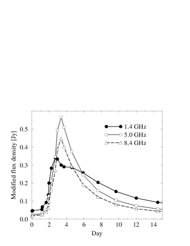
Figure 3: Model lightcurves at 1.4, 4.9, and 8.4 GHz for $P_{0}=200$ days, $\Omega_{0}=5\aas@@fstack{\circ}7$.

We can see that the model is capable of reproducing the observed time lag between 1.4 GHz and the higher radio frequencies. One can speculate that a more complex physical setting (e.g. spectral evolution of the underlying emission, or inhomogeneity of the emitting plasma) may be required for explaining the apparent discrepancy between the modeled and observed widths of the flare.

3.4 Free-free absorption by a foreground medium

Here we consider the effect of free-free absorption in a foreground medium, either in the host of the BL Lac object itself, or in one of the intervening redshift systems. To keep the discussion simple, we neglect the cosmological redshift, i.e., factors $(1+z)$. The optical depth for free-free absorption of a plasma is approximately given by (see e.g. Lang lang74 (1974)):

$$\tau=8.235\cdot 10^{-2}\,T^{-1.35}\,\nu^{-2.1}\,\int N^{2}\,dl\quad,$$ (4)

where $T$ is the electron temperature in K, $\nu$ is measured in GHz, and the emission measure $\int N^{2}\,dl$ in pc cm^-6. Thus, the absorption of radiation by a foreground medium can be described by $e^{-c\cdot\lambda^{2}}$, where $c$ is a constant. We assume the following scenario. The source is moving with transverse speed $v$ behind a patchy foreground medium so that changes in the emission measure towards the source produce variable absorption. To lowest order, we describe gaps between the clouds by

$$\tau=k^{2}\,\lambda^{2}\,x^{2}$$ (5)

($x$ being the axis perpendicular to the line of sight). Since the observed flux density of a point source is given by $S_{\rm obs}=S\,e^{-\tau}$, a moving source seen through such a gap in the foreground medium will show peaked lightcurves with roughly Gaussian shape. The width of the peaks will decrease with increasing wavelength. However, there are two major problems that need to be addressed. Firstly, in this model the maxima for all frequencies are reached at the same time, and secondly, the observed durations (i.e., the widths of the Gaussians fitted according to Equation (1)) do not follow the expected behavior $a_{4}\propto\lambda^{-1}$.

The time lags between the peaks of the observed lightcurves can be explained for an extended source by a slight shift of the brightness center depending on the frequency.

To deal with the second problem, we assume that the source is not point-like, but has a circular Gaussian shape, with the source size proportional to the wavelength. Thus, the flux density is given by

$$S(x,t)=S_{0}\cdot\exp\left(-\frac{(x-vt)^{2}}{\sigma_{\lambda}^{2}}\right)\quad,$$ (6)

with $\sigma_{\lambda}=\sigma_{0}\cdot\lambda$ (i.e., $\sigma_{0}$ is the source size at 1 m wavelength).

Assuming that the angular size of the variable region is much smaller than the antenna beam, the observed flux density is given by the integral

$$S_{\rm obs}(t)=\int^{+\infty}_{-\infty}S(x,t)\cdot e^{-\tau(x)}dx$$ (7)

Evaluating the above integral, gives (since $S_{\rm obs}$ is the integral of a product of two Gaussians)

$$S_{\rm obs}(t)=S^{\prime}\cdot\exp\left(\frac{-v^{2}t^{2}}{\sigma_{\lambda}^{2}+1/k^{2}\lambda^{2}}\right)$$ (8)

with a new normalization constant $S^{\prime}$. Therefore, the square of the width of the Gaussian is

$$a_{4}^{2}=\frac{1}{v^{2}}\left(\sigma_{\lambda}^{2}+\frac{1}{k^{2}\lambda^{2}}\right)=\frac{\sigma_{0}^{2}}{v^{2}}\lambda^{2}+\frac{1}{k^{2}\,v^{2}}\frac{1}{\lambda^{2}}\quad,$$ (9)

and it should depend on wavelength like $A\cdot\lambda^{2}+B\cdot\lambda^{-2}$. By adjusting the parameters $A$ and $B$ to fit the measured values of $a_{4}^{2}$ at the three observing wavelengths, we derive values for $\sigma_{0}^{2}/v^{2}$ and $k^{2}\cdot v^{2}$. We assume here that the transverse speed is dominated by superluminal motion with $v/c=\beta_{\rm app}$ and obtain a source size of $0.0067\cdot\beta_{\rm app}$ pc corresponding to an angular size of $1.6\cdot\beta_{\rm app}\,\mu$as at $\lambda=1$ m. We note that such a small source diameter even for $\beta_{\rm app}=10$ results in a brightness temperature of about $10^{15}$ K, and therefore violates the inverse Compton limit. For higher velocities – as observed in this source (e.g. Chu et al. chu96 (1996)) – the observed size can be larger. However, to reconcile our observational findings with the inverse Compton limit, Doppler factors of the order of 100 are needed.

The second term in Equation (9) gives the size of the gap in the foreground medium, i.e., the distance between the points where $\tau=1$. Since we assumed $\tau=k^{2}\,\lambda^{2}\,x^{2}$, this distance is $\Delta x=2/(k\cdot\lambda)$, which is about $2.3\cdot 10^{-4}\cdot\beta_{\rm app}$ pc at $\lambda=1$ m. (Note that this is true only for the case where the absorber is at the redshift of the BL Lac object; the ratio of the angular diameter distances of emitter and screen has to be applied as a correction factor in the case of an intervening absorber.)

We still have to check whether Equation (4) gives a sufficient optical depth for reasonable choices of electron temperature and emission measure. The strongest constraints come from the data at 3.6 cm: to explain the observed amplitude of 0.24 Jy at a source flux of 5 Jy, $\tau$ must be at least 0.05 at this wavelength. For an electron temperature of 5000 K, an emission measure of $5\cdot 10^{6}$ pc cm^-6 is needed. The thickness of the absorber cannot be much larger than the transverse scale derived above, which is 0.06 pc at 3.6 cm for $\beta_{\rm app}=10$; this gives an electron density of $10^{4}$ cm^-3. These values are within the range found in Galactic H II regions and planetary nebulae.

We conclude that this model can explain the observed shorter duration of the flares at longer wavelengths, and – under the assumption of slightly different spatial locations of the brightness center at the observed wavelengths – also the sequence of the peaks. It predicts that the amplitude of the peaks increases more strongly with wavelength than observed, but it is consistent with the data when an underlying non-variable component is taken into account. However, in the possible case of a connection between the radio and the optical variations this model fails, since the optical radiation would not be affected by free-free-scattering.

3.5 Interstellar scattering (ISS)

Scattering processes in the interstellar medium are well known to cause flux density variations at radio frequencies (e.g. Rickett rickett90 (1990)). In this section we investigate the possibility that ISS is the cause of the variations seen in our observations. We will follow mainly the considerations and notations of Rickett et al. (rickett95 (1995)). For a point-like source, the spatial scale of flux density variations caused by RISS is given by ($L$ is the path length through the medium, $\theta_{\mbox{\scriptsize scat}}$ the scattering angle)

$$r_{0,\lambda}\simeq 0.25\,L\,\theta_{\mbox{\scriptsize scat}}\quad,$$ (10)

which is proportional to $\lambda^{2.2}$, for a Kolmogorov-type medium (Rickett et al. rickett84 (1984)), and therefore also $\theta_{\mbox{\scriptsize scat}}\propto\lambda^{2.2}$ (cf. Cordes et al. cordes84 (1984)). The spatial scale of an extended source (assuming a Gaussian shape of $\sigma_{\lambda}$ in width) is then given by

$$r_{\theta,\lambda}=\sqrt{r^{2}_{0,\lambda}+(0.5\,L\,\sigma_{\lambda})^{2}}\quad.$$ (11)

Then, the scintillation index $m_{\theta,\lambda}$ and the variability timescale $\tau_{\theta,\lambda}$ for the extended source can be derived by

$$m_{\theta,\lambda} = m_{0,\lambda}\frac{r_{0,\lambda}}{r_{\theta,\lambda}}\quad,$$ (12)

$$\tau_{\theta,\lambda} = \frac{r_{\theta,\lambda}}{V}\quad,$$

where $V$ is the velocity of the Earth (i.e., the observer) relative to the scattering medium, and $m_{0,\lambda}$ is the (wavelength dependent) scintillation index of a point source.

We assume a source diameter which is proportional to $\lambda$ as we did in the previous section, thus $\sigma_{\lambda}=\sigma_{0}\lambda$, and use $\theta_{\mbox{\scriptsize scat}}=\theta_{0}\lambda^{2.2}$ (see above). This gives

$$m_{\theta,\lambda} = \frac{m_{0,\lambda}\,\theta_{0}\,\lambda^{2.2}}{\sqrt{\theta_{0}^{2}\,\lambda^{4.4}+4\,\sigma_{0}^{2}\,\lambda^{2}}}\quad\mbox{and}$$ (13)

$$\tau_{\theta,\lambda} = \frac{L}{4V}\sqrt{\theta_{0}^{2}\,\lambda^{4.4}+4\,\sigma_{0}^{2}\,\lambda^{2}}\quad.$$

Therefore, it is clear that – independent of the wavelength dependence of $m_{0,\lambda}$ – the timescales of the variations become shorter for decreasing wavelengths. This is contrary to our observational findings (see Table 1), implying that this simple model is unlikely to explain the observations. Additionally, interstellar scattering cannot cause variability in the optical regime. Hence, in this case again, a possible connection of the optical and the radio variations would rule out ISS as the only cause of the observed variability.

However, owing to the small source diameters involved here, ISS can be present as an additional effect. As an example, we calculate the scintillation index and the timescales with the following assumptions. Following Rickett (rickett86 (1986)) the path length in the interstellar medium of our galaxy is $L\simeq 500\,{\rm pc}\cdot\csc|b|\simeq 788\,{\rm pc}$ (the source galactic latitude is $-40^{\circ}$). With $\sigma_{0}=1.2$ mas (which corresponds to $T_{\rm B}\simeq 10^{12}$ K), $\theta_{0}=60$ mas and a typical velocity (of the observer) $V=50$ km/s this yields:

$\lambda$ [cm]	$m_{\theta,\lambda}$	$\tau_{\theta,\lambda}$ [d]
20	0.48	12.2
6	0.32	1.28
3.6	0.21	0.64

Therefore, the faster variations which are clearly seen at higher frequencies (especially in the 6 cm lightcurve) may be due to ISS.

3.6 Gravitational Microlensing

Another possible explanation for the origin of the observed variations is gravitational microlensing (ML) by stars in a foreground galaxy. ML effects have been unambiguously observed in the multiple QSO 2237+0305 (Irwin et al. irwin89 (1989), Houde & Racine houde94 (1994)), and most likely also in other multiply-imaged QSOs (see Wambsganss wambsganss93 (1993), and references therein). The possibility that ML can cause AGN variability has long been predicted (Paczyński paczynski86 (1986), Kayser et al. kayser86 (1986), Schneider & Weiss schneider87 (1987)), but it remains unclear whether ML causes a substantial fraction of the observed variability in QSOs (e.g. Schneider schneider93 (1993)).

0235+164 has a foreground galaxy ($z=0.524$) situated within two arcseconds from the line of sight (Spinrad & Smith spinrad75 (1975)), and an additional galaxy 0$\aas@@fstack{\prime\prime}$5 away from the source (Stickel et al. stickel88 (1988), see also additional components reported in Yanny et al. yanny89 (1989)). Additionally, a nearby absorption system was observed at $\lambda=21$ cm by Wolfe, Davis & Briggs (wolfe82 (1982)). All three objects may host microlenses affecting the emission from 0235+164. Thus, for 0235+164 the probability for ML is expected to be high (Narayan & Schneider narayan90 (1990)), so that sometimes ML events should be present in the lightcurves.

We will show now how ML can modulate the underlying long-term lightcurve and explain faster variations of long-wavelength flux compared to short-wavelength radiation, even when the longer wavelength radiation comes from a larger source (component). Since the available data do not permit a detailed account of possible ML situations, the attention here is restricted to two simple situations: an isolated point-mass lens in the deflector, and a cusp singularity, formed by an ensemble of microlenses (Schneider & Weiss schneider87 (1987), Wambsganss wambsganss90 (1990)). In fact, both cases yield similar predicted ML lightcurves. The scales of the source size and the lens mass necessary to yield a flux variation of the observed kind can be estimated for both cases together.

We assume an elliptically shaped emitting feature that moves relativistically in the direction roughly coinciding with the minor axis of the ellipse. Such a component can be formed by relativistic electrons which are locally accelerated by a shock front inside a superluminal jet. The shape of the source component and its orientation is then determined by the flow inside the jet. A Gaussian brightness profile is assumed, with component size $\propto\lambda$ (see Fig. 4 for details). We postulate that the emission peaks at all three wavelengths are displaced relative to each other, but that the peaks of shorter-wavelength components are situated within the half intensity contour of longer-wavelength components.

Let $\beta c$ be the apparent effective transverse velocity of the source component; using the redshift $z_{s}=0.94$ of the object, this corresponds to an angular velocity of $v_{\rm a}=2\beta h\,10^{-4}$ mas/day. If a source component moves along a track in the source plane, and the component size is much smaller than the minimum angular separation $d_{\rm a}$ from the singularity, as indicated in Fig. 4 (solid ellipse), then the timescale of variation is given roughly by the ratio $d_{\rm a}/v_{\rm a}$. On the other hand, if a strongly elongated source component moves so that parts of it cross the line of sight to the singularity (as indicated in Fig. 4, dashed ellipse), then the shortest possible timescale is roughly the ratio between the transverse angular source size $a_{\lambda}$ (the minor semi-axis at wavelength $\lambda$) and the angular velocity. Now assume that the former case approximates the 3.6 cm source and the latter case approximates the 20 cm source. If $\Delta t_{3.6}\sim 4$ days, $\Delta t_{6}\sim 3$ days and $\Delta t_{20}\sim 2$ days are the variability timescales for the three wavelengths considered, we have

$$d_{\rm a}\sim v_{\rm a}\,\Delta t_{3.6}\sim 8\beta h\,10^{-4}{\,\rm mas}\quad,$$ (14)

and

$$r\,a_{20}\sim 4\beta h\,10^{-4}\;{\rm mas}\quad,$$ (15)

where $r\leq 1$ is the axis ratio of the Gaussian source component. In order for the 20 cm source to experience appreciable variations, the closest separation of its center from the singularity cannot be larger than its major semi-axis, i.e., $a_{20}\mathrel{\mathchoice{\lower 2.0pt\vbox{\halign{$\m@th\displaystyle\hfil#\hfil$\cr>\crcr\sim\crcr}}}{\lower 2.0pt\vbox{\halign{$\m@th\textstyle\hfil#\hfil$\cr>\crcr\sim\crcr}}}{\lower 2.0pt\vbox{\halign{$\m@th\scriptstyle\hfil#\hfil$\cr>\crcr\sim\crcr}}}{\lower 2.0pt\vbox{\halign{$\m@th\scriptscriptstyle\hfil#\hfil$\cr>\crcr\sim\crcr}}}}d_{\rm a}$, and this inequality can be satisfied for $r\mathrel{\mathchoice{\lower 2.0pt\vbox{\halign{$\m@th\displaystyle\hfil#\hfil$\cr<\crcr\sim\crcr}}}{\lower 2.0pt\vbox{\halign{$\m@th\textstyle\hfil#\hfil$\cr<\crcr\sim\crcr}}}{\lower 2.0pt\vbox{\halign{$\m@th\scriptstyle\hfil#\hfil$\cr<\crcr\sim\crcr}}}{\lower 2.0pt\vbox{\halign{$\m@th\scriptscriptstyle\hfil#\hfil$\cr<\crcr\sim\crcr}}}}0.5$.

Figure 4: Geometry of the proposed microlensing scenario. Elliptical surface brightness contours are drawn for the 3.6 cm (solid), 6 cm (dotted), and 20 cm (dashed) source components. The caustic point of the microlens is at the origin, denoted by ‘X’, and the source components are assumed to move along the solid line as indicated. The scales indicated on the axis correspond to the synthetic lightcurves shown in Fig. 5.

Since the relative contribution of the moving component to the total flux of the source is unknown, we cannot use the observed lightcurves to determine the magnification of the component emission. The magnification of a point source at separation $\theta$ from the point singularity is

$$\mu_{\rm p}={x^{2}+2\over x\sqrt{x^{2}+4}}\quad,$$ (16)

where $x=\theta/\theta_{0}$, and $\theta_{0}$ is the angular scale induced by a point mass lens of mass $M$:

$$\theta_{0}=\sqrt{{4GM\over c^{2}}{D_{\rm ds}\over D_{\rm s}D_{\rm d}}}\quad,$$ (17)

where $D_{\rm d}$, $D_{\rm s}$, and $D_{\rm ds}$ denote, respectively, the angular diameter distances to the lens, the source, and from the lens to the source, $m=M/M_{\odot}$ is the lens mass in units of the solar mass. Assuming that the lens is situated at $z=0.525$,

$$\theta_{0}=1.87\sqrt{mh}\,10^{-3}\;{\rm mas}\quad.$$ (18)

Approximating the point-source magnification by $\mu_{\rm p}\simeq 1/x$ (for $x\ll 1$), and assuming as before that the size $a_{3.6}$ is much smaller than the closest separation of the source from the point-like singularity, the maximum magnification of this source component becomes

$$\mu_{\rm 3.6,max}\sim{\theta_{0}\over d_{\rm a}}\simeq 2.34\,m^{1/2}\,h^{-1/2}\,\beta^{-1}\quad.$$ (19)

Hence, a solar-mass star would yield a magnification of the order of 2 for the smallest source component moving at roughly the speed of light and in general can produce lightcurves similar to the observed variations.

In Fig. 5, we plot numerically determined ML lightcurves for a moving source with an axis ratio $r=0.4$, minimum separation $d_{\rm a}=8\beta h10^{-4}$ mas, and semi-major axis of the 20 cm source component of $a_{20}=\beta h10^{-3}$ mas. The lens mass is $m=0.4\beta^{2}h$. The source sizes are chosen to be proportional to wavelength, and the brightness peaks of the 6 cm and 20 cm components are displaced relative to the peak of the 3.6 cm component by 0.4 of their corresponding sizes. As can be seen from the modeled lightcurves, the variability timescale of the 20 cm component is considerably shorter than that of the shorter wavelength components, in accordance with our analytical estimates. In addition, the observed shift of the brightness peak at 20 cm before those at smaller wavelengths can be accounted for in our model by a slight tilt of the direction of motion of the source relative to the minor axis of the surface brightness ellipses, in the sense of the large component crossing the caustic point before the closest approach of the 3.6 cm component to that point. Nevertheless, we note that the small source sizes needed (in the range of $\mu$as) will result in brightness temperatures of the order of $10^{15}$ K, i.e., three orders of magnitude above the inverse Compton limit.

Figure 5: Microlensing lightcurves obtained from the model discussed in the text. The three curves correspond to the 3.6 cm (solid), 6 cm (dotted) and 20 cm (dashed) source components.

A more detailed modeling of the lightcurves by a microlensing scenario is not warranted at this stage, given the large number of degrees of freedom. Nevertheless, the above considerations have demonstrated that the basic qualitative features can be understood in the microlensing picture without very specific assumptions.

4 Conclusions

We have observed the BL Lac object 0235+164 at three radio wavelengths and in the optical R-band and found rapid variations in all frequency bands. One single event that can be identified at all radio wavelengths shows very peculiar properties. The brightness peak is reached first at 20 cm wavelength, and afterwards at 3.6 and 6 cm. The amplitudes of the flares decrease from longer to shorter radio wavelengths, and the timescales become longer. The event in the radio regime might be connected to the bright peak in the optical lightcurve, although this connection remains questionable due to the sparse sampling of the R-band data. In the previous sections, we have discussed some models and to what extent they can explain the observed variations.

While the conventional application of the shock-in-jet model has difficulties in reproducing the observations, the assumption of an increasing optical depth (e.g. due to continuous injection of relativistic electrons) can cause a delay of the maximum at high frequencies with respect to the lower frequencies, and therefore explain at least one of the special features.

Variable Doppler boosting can cause simultaneous short-term variability in all observed wave bands. Fairly pronounced time lags between the different frequencies can be caused by turnover frequency variations in the observed spectrum of a moving source. However, broader peaks are expected at longer wavelengths.

Free-free absorption and interstellar scattering are only capable of explaining radio variations, not variability in the optical regime. Therefore, if the connection between the optical and the radio variability is real, these models are ruled out as the only cause for the variations. Furthermore, the dependence of the timescales on wavelength argues against an explanation of the flare by interstellar scattering. The absorption by a patchy foreground medium can easily describe the shape and the widths of the flares (in the radio) and can – if we assume different locations for the brightness center – also explain the time sequence of the brightness peaks.

Gravitational Microlensing – in combination with a wavelength-dependent source size and a slight displacement of the brightness peak – provides a possible explanation for the observed variations in the radio regime. One would also expect fairly strong variability in the visible range, because of the much smaller source size. Microlensing thus appears to be a viable explanation of the observations, which is also quite attractive because of the known foreground objects.

It is quite remarkable that these attempts to explain the rapid radio variability in 0235+164 – different as they are – all imply that the intrinsic source size is very small. To reconcile the observations with the 10¹² K inverse Compton limit, a Doppler factor substantially higher than the “canonical” value of 10 (see e.g. Ghisellini et al. 1993, Zensus 1997) is required. Most scenarios that we have investigated imply ${\cal D}\simeq 100$. In this context it is interesting to note that circumstantial evidence for superluminal motion with $\beta_{\rm app}\sim 30$ has been found in this source (Chu et al. 1996). The variations in 0235+164 are also among the strongest and fastest of all sources in the Michigan monitoring program (e.g. Hughes et al. 1992). This suggests that the distribution of Doppler factors in compact radio sources has a tail extending to ${\cal D}\simeq 100$, and that 0235+164 – and perhaps more generally the sources showing strong intraday radio variability – belong to this tail. The implied extremely small source size can allow rapid intrinsic variations, and at the same time favor propagation effects. It is therefore plausible that the observed variability is caused by a superposition of both mechanisms.

- (1) Abraham, R.G., Crawford, C.S., Merrifield, M.R., et al., 1993, ApJ 415, 101
- (2) Aller, M.F. 1999, In: Takalo, L. & Valtaoja, E. (eds.) BL Lac phenomenon. ASP conference series, in press
- (3) Baars, J.W.M., Genzel, R., Pauliny-Toth, I.I.K., Witzel, A., 1977, A&A 61, 99
- (4) Bååth, L.B., 1984, VLBI Monitoring of BL Lac Objects. In: Fanti, R., Kellermann, K., Setti, G. (eds.) VLBI and Compact Radio Sources. IAU Symp. 110, Reidel, Dordrecht, 127
- (5) Blandford, R.D., Königl, A., 1979, ApJ 232, 34
- (6) Burbidge, E.M., Beaver, E.A., Cohen, R.D., et al., 1996, AJ 112, 2533
- (7) Camenzind, M., Krockenberger, M., 1992, A&A 255, 59
- (8) Chu, H.S., Bååth, L.B., Rantakyrö, F.T., et al., 1996, A&A 307, 15
- (9) Cohen, R.D., Smith, H.E., Junkkarinen, V.T., Burbidge, E.M., 1987, ApJ 318, 577
- (10) Cordes, J.M., Ananthakrishnan, S., Dennison, B., 1984, Nature 309, 689
- (11) Crane, P.C., Napier, P.J., 1989: Sensitivity, In: Synthesis Imaging in Radio Astronomy, Perley, R.A., Schwab, F.R., Bridle, A.H. (eds.), ASP Conf. Ser. 6, 139
- (12) Ghisellini, G., Padovani, P., Celotti, A., Maraschi, L., 1993, ApJ 407, 65
- (13) Heidt, J., Wagner, S.J., 1996, A&A 305, 42
- (14) Houde, M., Racine, R., 1994, AJ 107, 466
- (15) Hughes, P.A., Aller, H.D., Aller, M.F., 1992, ApJ 396, 469
- (16) Irwin, M.J., Hewett, P.C., Corrigan, R.T., et al., 1989, AJ 98, 1989
- (17) Jones, D.L., Unwin, S.C., Bååth, L.B., Davis, M.M., 1984, ApJ 284, 60
- (18) Kayser, R., Refsdal, S., Stabell, R., 1986, A&A 166, 36
- (19) Kellermann, K.I., Pauliny-Toth, I.I.K., 1969, ApJ 155, L71
- (20) Lang, K.R., 1974, Astrophysical Formulae, Springer-Verlag, Berlin, Heidelberg
- (21) Madejski, G., Takahashi, T., Tashiro, M., et al., 1996, ApJ 459, 156
- (22) Marscher, A.P., 1990, Interpretation of Compact Jet Observations. In: Zensus, J.A., Pearson, T.J. (eds.) Parsec-Scale radio jets. Cambridge University Press, Cambridge, 236
- (23) Marscher, A.P., Gear, W.K., 1985, ApJ 298, 114
- (24) v. Montigny, C., Bertsch, D.L., Chiang, J., et al., 1995, ApJ 440, 525
- (25) Narayan, R., Schneider, P., 1990, MNRAS 243, 192
- (26) Nilsson, K., Charles, P.A., Pursimo, T., et al., 1996, A&A 314, 754
- (27) O’Dell, S.L., Dennison, B., Broderick, J.J., et al., 1988, ApJ 326, 668
- (28) Ott, M., Witzel, A., Quirrenbach, A., et al., 1994, A&A 284, 331
- (29) Pacholczyk, A.G., 1977, Radio Galaxies, Pergamon Press, Oxford
- (30) Paczyński, B., 1986, ApJ 301, 503
- (31) Qian, S.J., Li, X.C., Wegner, R., et al., 1996, Chin. Astron. Astroph. 20, 15
- (32) Quirrenbach, A., Witzel, A., Krichbaum, T.P., et al., 1992, A&A 258, 279
- (33) Rabbette, M., McBreen, B., Steel, S., Smith, N., 1996, A&A 310, 1
- (34) Rickett, B.J., 1986, ApJ 307, 564
- (35) Rickett, B.J., 1990, ARAA 28, 561
- (36) Rickett, B.J., Coles, W.A., Bourgois, G., 1984, A&A 134, 390
- (37) Rickett, B.J., Quirrenbach, A., Wegner, R., et al., 1995, A&A 293, 479
- (38) Roland, J., Teyssier, R., Roos, N., 1994, A&A 290, 357
- (39) Romero, G.E., Combi, J.A., Benagli, P., et al., 1997, A&A 326, 77
- (40) Schneider, P., 1993, A&A 279, 1
- (41) Schneider, P., Weiss, A., 1987, A&A 171, 49
- (42) Schramm, K.-J., Borgeest, U., Kuehl, D., et al., 1994, A&AS 106, 349
- (43) Shen, Z.-Q., Wan, T.-S., Moran, J.M., et al., 1997, AJ 114, 1999
- (44) Smith, H.E., Burbidge, E.M. & Junkkarinen, V.T., 1977, ApJ 218, 611
- (45) Spinrad, H., Smith, H.E., 1975, ApJ 201, 275
- (46) Stevens, J.A., Litchfield, S.J., Robson, E.I., et al., 1994, ApJ 437, 91
- (47) Stickel, M., Fried, J.W., Kühr H., 1988, A&A 198, L13
- (48) Takalo, L.O., Kidger, M.R., de Diego, J.A., et al., 1992, AJ 104, 40
- (49) Teräsranta, H., Tornikoski, M., Valtaoja, E. et al., 1992, A&AS 94, 121
- (50) Wagner, S.J. & Witzel, A., 1995, ARAA 33, 163
- (51) Wambsganss, J.: 1990, Gravitational Microlensing. In: MPA Report 550, MPA (Garching)
- (52) Wambsganss, J., 1993. In: Surdej, J., Fraipont-Crao, D., Gosset, E., Refsdal, S., & Remy, M. (eds.), Gravitational Lenses in the Universe, Universite de Liege, 369
- (53) Webb, J.R., Smith, A.G., Leacock, R.J. et al., 1988, AJ 95, 374
- (54) White, R.J., Peterson, B.M., 1994, PASP 106, 879
- (55) Wolfe, A.M., Davis, M.M., Briggs, F.H., 1982, ApJ 259, 495
- (56) Yanny, B., York, D.G., Gallagher, J.S., 1989, ApJ 338, 735
- (57) Zensus, J.A., 1997, ARAA 35, 607