On the transfer of momentum from stellar jets to molecular outflows

Abstract

While it is generally thought that molecular outflows from young stellar objects (YSOs) are accelerated by underlying stellar winds or highly collimated jets, the actual mechanism of acceleration remains uncertain. The most favoured model, at least for low and intermediate mass stars, is that the molecules are accelerated at jet-driven bow shocks. Here we investigate, through high resolution numerical simulations, the efficiency of this mechanism in accelerating ambient molecular gas without causing dissociation. The efficiency of the mechanism is found to be surprisingly low suggesting that more momentum may be present in the underlying jet than previously thought. We also compare the momentum transferring efficiencies of pulsed versus steady jets. We find that pulsed jets, and the corresponding steady jet with the same average velocity, transfer virtually the same momentum to the ambient gas. The additional momentum ejected sideways from the jet beam in the case of the pulsed jet only serves to accelerate post-shock jet gas which forms a, largely atomic, sheath around the jet beam.

For both the steady and pulsing jets, we find a power law relationship between mass and velocity ($m(v)\propto v^{-\gamma}$) which is similar to what is observed. We also find that increasing the molecular fraction in the jet decreases $\gamma$ as one might expect. We reproduce the so-called Hubble law for molecular outflows and show that it is almost certainly a local effect in the presence of a bow shock.

Finally, we present a simple way of overcoming the numerical problem of negative pressures while still maintaining overall conservation of energy.

1 Introduction

It has been proposed that molecular outflows, at least from low and intermediate mass young stars, may be driven by highly collimated jets (see, for example, Padman, Bence & Richer PBR (1997)). Although the likely mechanism by which such jets transfer their momentum to the ambient medium remains unknown, a number of ideas have been put forward (for a review of models the reader is referred to Cabrit, Raga & Gueth CRG (1997)). Of these the most promising seems to be the so-called “prompt entrainment” mechanism. According to this model the bulk of the molecular outflow is accelerated ambient gas near the head of the jet or more precisely along the wings of its associated bow shock. Observational support for prompt entrainment comes from the spatial coincidence of shocked molecular hydrogen bows with peaks in the CO outflow emission (e.g. Davis & Eislöffel D&E (1995)).

Smith, Suttner & Yorke (smith (1997)) and Suttner et al. (Suttner (1997)) have carried out a number of 3-D simulations of dense molecular jets propagating into a dense medium in order to test the prompt entrainment hypothesis. These authors found that their simulations reproduced many of the observational characteristics of molecular flows including the so-called ‘Hubble law’ (see, e.g. Padman et al. PBR (1997)) and strong forward, as opposed to sideways, motion (Lada & Fich LF (1996)). While such results are encouraging for jet-driven models, it is still fair to say that no individual model has yet been able to plausibly account for all the observations (Lada & Fich LF (1996)). Moreover, alternatives to the jet model may be better at explaining the observational characteristics of some molecular flows (e.g. Padman et al. PBR (1997) and Cabrit et al. CRG (1997)).

The limited resolution of the 3-D jet simulations of Smith et al. (smith (1997)), and Suttner et al. (Suttner (1997)), along with the high densities used by these authors, meant that they could not resolve the post-shock cooling regions in the flow. In addition it was not possible to explore parameter space as only a few such simulations could be performed. Here we take a somewhat different approach by assuming low density atomic/molecular jet mixtures, a low density ambient medium and cylindrical symmetry. Although such an approach obviously has it limitations, it does allow us to explore parameter space more fully and to resolve post-shock cooling regions (this might be important, for example, if one is to gauge the importance of certain instabilities). The primary goal of this work is to investigate the efficiency of YSO jets in accelerating ambient molecular gas without causing dissociation of its molecules.

An additional question we address in this paper is whether velocity variations (pulsing) of the jet might enhance transfer of momentum from the jet to its surroundings and thus help to accelerate ambient gas. Pulsing induces internal shocks which can squeeze jet gas sideways (Raga et al. Retal93 (1993)). This gas does not interact with the ambient medium directly, but is instead squirted into the cocoon of processed (post-shock) jet gas, which separates the jet from the “shroud” of post-shock ambient gas. Chernin & Masson (C&M (1995)) however argue that, through the cocoon, momentum from the jet may be continuously coupled to the ambient flow.

The properties of the simulated systems in which we are interested are as follows:

• How much momentum is transferred to the ambient molecules?

• Is there a power-law relationship predicted between mass in the molecular flow and velocity?

• What are the proper motions of the molecular ‘knots’, and how does their emission behave with time?

• Is the so-called ‘Hubble law’ of molecular outflows reproduced under reasonable conditions?

• Is there extra entrainment of ambient gas along the jet due to velocity variations?

We will discuss each of these points in turn when presenting our results.

Our numerical model is presented in §2 and our results in §3. Conclusions from this work are presented in §4 and a simple way of overcoming the numerical problem of negative pressures while still maintaining overall energy conservation is given in the Appendix.

2 Numerical model

2.1 Equations and numerical method

The equations solved are

$$\frac{\partial\rho}{\partial t} = -\@vec{\nabla}\cdot(\rho\@vec{u})$$ (1)

$$\frac{\partial\left(\rho\@vec{u}\right)}{\partial t} = -\@vec{\nabla}\cdot[\rho\@vec{u}\@vec{u}+P\@vec{\@vec{I}}]$$ (2)

$$\frac{\partial e}{\partial t} = -\@vec{\nabla}\cdot\left[\left(e+P\right)\@vec{u}\right]-L$$ (3)

$$\frac{\partial n_{\rm H}x}{\partial t} = -\@vec{\nabla}\cdot\left[n_{\rm H}x\@vec{u}\right]+J(x,n_{\rm H},T)$$ (4)

$$\frac{\partial n_{\rm H_{2}}}{\partial t} = -\@vec{\nabla}\cdot(n_{\rm H_{2}}\@vec{u})-n_{\rm H_{2}}n_{\rm H}k(T)$$ (5)

$$\frac{\partial n_{\rm H}}{\partial t} = -\@vec{\nabla}\cdot(n_{\rm H}\@vec{u})+2n_{\rm H_{2}}n_{\rm H}k(T)$$ (6)

$$\frac{\partial\rho\tau}{\partial t} = -\@vec{\nabla}\cdot(\rho\tau\@vec{u})$$ (7)

where $\rho$, $\@vec{u}$, $P$, $e$ and $I$ are the mass density, velocity, pressure, total energy density and identity matrix respectively. $n_{\rm H}$ and $n_{\rm H_{2}}$ are the number densities of atomic and molecular hydrogen, $x$ is the ionization fraction of atomic hydrogen, $T$ is the temperature, $J(x,n_{\rm H},T)$ is the ionization/recombination rate of atomic hydrogen, $k(T)$ is the dissociation coefficient of molecular hydrogen, and $\tau$ is a passive scalar which is used to track the jet gas. We also have the definitions

$$e = \frac{1}{2}\rho\@vec{u}\cdot\@vec{u}+\frac{c_{v}}{k_{\rm B}}P$$ (8)

$$L = L_{\rm rad}+E_{\rm I}J(x,n_{h},T)+E_{\rm D}k(T)$$ (9)

where $c_{v}$ is the specific heat at constant volume, $k_{\rm B}$ is Boltzmann’s constant, $E_{\rm I}$ is the ionization energy of hydrogen and $E_{\rm D}$ is the dissociation energy of H₂. So $L$ is a function which denotes the energy loss and gain due to radiative and chemical processes. $L_{\rm rad}$ is the loss due to radiative transitions and is made up of a function for losses due to atomic transitions (Sutherland & Dopita S&D (1993)), and one for losses due to molecular transitions (Lepp & Shull L&S (1983)). The second term in $L$ is the energy dumped into ionization of H, and the third is that dumped into dissociation of H₂. The dissociation coefficient $k(T)$ is obtained from Dove & Mandy (D&M (1986)) and the ionization rate, $J$, is that used by Falle & Raga (F&R (1995)).

These equations are solved in a 2D cylindrically symmetric geometry using a temporally and spatially second order accurate MUSCL scheme (van Leer leer (1977); Falle falle (1991)). The code uses a linear Riemann solver except where the resolved pressure differs from either the left or right state at the cell interface by greater than 10% where it uses a non-linear solver (following Falle 1996, private communication). Non-linear Riemann solvers allow correct treatment of shocks and rarefactions without artificial viscosity or entropy fixes. Applying them only in non-smooth regions of the flow means that, while the benefits are the same, the computational overhead is minimised. This code is an updated version of that described in Downes & Ray (D&R (1998)).

Sometimes negative pressures are predicted by simulations involving radiative cooling. Typically these are overcome by simply resetting the calculated pressure to an arbitrary, but small, positive value. However, this involves injecting internal energy into the system and this is undesirable. A fairly reliable way of overcoming this problem is discussed in Appendix A.

2.2 Initial conditions

Initially the ambient density and pressure on the grid are uniform and defined so that the ambient temperature on the grid is $10^{2}$ K. The jet temperature is set to $10^{3}$ K. The function $L$ is set to zero below this latter temperature as the data used in the cooling functions becomes unreliable and cooling below this temperature is not dynamically significant anyway. In most cases the ratio of jet density to ambient density ($\equiv\eta$) is set to 1 (see Table 1). The ratio $\frac{n_{\rm H_{2}}}{n_{\rm H}}=9$ both inside and outside the jet, unless otherwise indicated (again, see Table 1). In all cases the gas is assumed to be one of solar abundances. The boundary conditions are reflecting on $r=0$ (i.e. the jet axis) and on $z=0$ except where the jet enters, and gradient zero on every other boundary. The computational domain measures $1500\times 300$ cells (but larger in the $\eta=10$ simulations), with a spacing of $1\times 10^{14}$ cm. We find that the efficiency of momentum transfer is sensitive to the grid spacing. We performed a number of simulations with different spacings and concluded that this is the absolute minimum necessary to get reliable results. This length should be reduced with increasing density. Incidentally this means that examining this property at the densities used by, for example, Smith et al. (smith (1997)) is impractical.

The jet enters the grid at $z=0$ and $r\leq R$ and the boundary conditions are set to force inflow with the jet parameters. $R$ is set at $5\times 10^{15}$ cm or 50 grid cells. The jet velocity is given by

$$v_{\rm jet}(t)=v_{0}+\frac{v_{1}}{4}\sum_{j=1}^{4}\sin(\omega_{j}t)$$ (10)

with $v_{0}\approx 215$ km s^-1 corresponding to a Mach number of 65 and $\omega_{j}$ are chosen so that the corresponding periods are 5, 10, 20 and 50 yrs. Here $v_{1}$ is effectively an amplitude for the velocity variations where present. The jet is initially given a small shear layer of about 5 cells ($5\times 10^{14}$ cm) in order to avoid numerical problems at the boundary between the jet and ambient medium. In this layer the velocity decays linearly to zero.

Nine simulations were run with varying values of density and velocity perturbation. These are listed in Table 1 which also gives the key we will use to refer to the simulations. In addition simulations of a purely atomic jet, and of a jet with a wide shear layer of almost 25 cells ($2.5\times 10^{15}$ cm) were run. The velocity of the jet with the wide shear layer is given by

$$v_{\rm jet}(t,r)=\frac{v_{\rm jet}(t)}{2}\left\{1-\tanh\left(\frac{r-R}{10^{15}\rm{cm}}\right)\right\}$$ (11)

where $v_{\rm jet}(t)$ is given by Eq. 10. Each system was simulated to an age of 300 yrs. Although this is very young compared to the observed age of stellar jets, it was felt that the qualitative behaviour of the system at longer times could reliably be inferred from these results. The densities chosen are rather low to ensure adequate resolution of the system as described above. Unfortunately this precludes the use of the data of McKee et al. (mckee (1982)) for calculations of the emissions from CO as their calculations are only valid for gases of much higher densities. As a result we present our findings in terms of the mass of molecular gas rather than its luminosity.

Label	Jet density (cm-3)	($\frac{v_{1}}{v_{0}}$)	Notes
A	10	0	-
B	10	0.6	-
C	100	0	-
D	100	0.1	-
E	100	0.2	-
F	100	0.4	-
G	100	0.6	-
G1	100	0.6	Wide shear layer
G2	100	0.6	Atomic jet
H	100	0.0	$\eta=10$
I	100	0.6	$\eta=10$

Table 1: A list of the simulations performed in this work. Unless otherwise stated $\eta=1$

3 Results

Fig. 1 shows plots of the distribution of number density for simulations C and G. The cocoon of the varying jet has many bow-shaped shocks travelling through it as a result of the internal working surfaces in the jet forcing gas and momentum out of the jet beam. It is interesting to note that the bow shock of the steady jet is more irregular than that of the pulsed jet. This irregularity is probably due to the Vishniac instability (e.g. Dgani et al. dgani (1996)) growing at the head of the jet. Presumably the variation of the conditions at the head of the varying jet dampens the growth of this instability. It should be noted that the enforced axial symmetry in these calculations makes the bow shock appear more smooth than it would in 3D simulations. However, the phenomenon of the bow shock breaking up occurs in both 2D and 3D simulations.

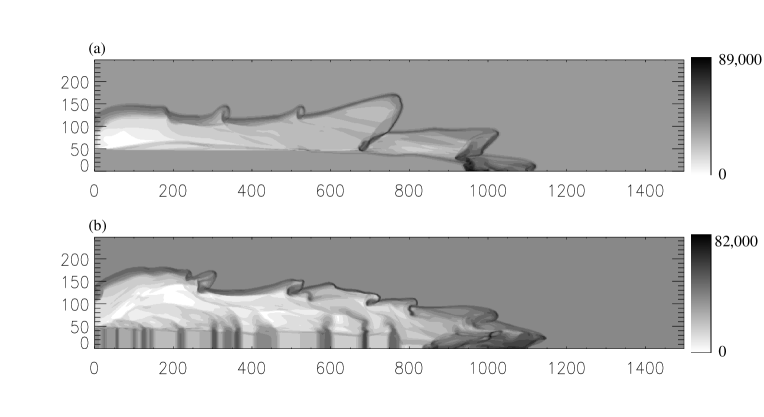
Figure 1: Log-scale plots of the distribution of number density for (a), simulation C, and (b), simulation G at $t=300$ yrs. The scales are in units of cm^-3

We will discuss each of the properties mentioned in §1 below.

3.1 Momentum transfer

We make use of the jet tracer $\tau$ to track how much momentum has been transferred from the jet to the ambient medium. The fraction of momentum transferred from jet gas to ambient molecules is

$${\cal F}_{\rm H_{2}}=\frac{\sum_{i,j}(1-\tau_{ij})|\@vec{u}_{ij}|m_{\rm H_{2}}n_{{\rm H_{2}},ij}dV_{ij}}{\sum_{i,j}|\@vec{u}_{ij}|n_{ij}<m>dV_{ij}}$$ (12)

where $n_{{\rm H_{2}},ij}$ and $n_{ij}$ are the number density of molecular hydrogen and the total number density in cell $ij$ respectively, $i$ and $j$ are cell indices in the $z$ and $R$ directions, and $dV_{ij}$ is the volume of cell $ij$. This equation is valid since the only momentum on the grid originated in the jet, and since the simulations are stopped before any gas flows off the grid. Note that we only consider momentum transferred to ambient molecules because we are only interested in how efficient YSO jets are at accelerating molecules, not atoms. Thus we ignore ambient molecules which have been dissociated in the acceleration process. Table 2 shows the fraction of momentum in ambient molecules for all the simulations after 300 yrs. For completeness we also show ${\cal F}_{\rm total}$, the total fraction of momentum transferred to ambient gas, whether molecular or atomic.

The first interesting point to note from Table 2 is that the amount of momentum residing in ambient molecules in these simulations is typically an order of magnitude less than the total momentum contained on the grid. Note, however, how significant amounts of momentum are transferred to the ambient medium as a whole, especially in those cases where the jet density matches that of its environment. This is as one would expect. What is perhaps surprising at first is the low efficiency of momentum transfer to ambient gas that remains in molecular form in the post-bow shock zone.

Comparison between ${\cal F}_{\rm total}$ and ${\cal F}_{\rm H_{2}}$ for models A and C and models B and G clearly shows that the momentum transfer efficiency from the jet to the ambient medium decreases with increasing density. This result is particularly marked in the case of post-shock ambient molecules. Although further simulations should be performed to confirm this finding, it is physically plausible. Cooling causes the bow shock to be narrower (i.e. more aerodynamic) than in the adiabatic case, thus reducing its cross-sectional area. Obviously this leads to a reduction in rate at which momentum is transferred from the jet to its surroundings. The fact that the effect is more marked for post-shock ambient molecules must reflect changes in the shape of the bow (as opposed to pure changes in its cross sectional area) with increased cooling.

Since we are simulating systems here which are probably of low density in comparison to typical YSO jets, our results suggest that radiative bow shocks, from at least heavy and equal density jets (with respect to the environment), are not very good at accelerating ambient molecules without causing dissociation. This result also points to the fact that in the case of such jets, the jet may carry much more momentum than one might naively estimate based on a rough balance with the momentum in any associated observed molecular flow.

We now turn to differences in the efficiency of momentum transfer in pulsed versus steady jets. The topic of differences in entrainment rates will be discussed more fully in §3.5. Fig. 2 shows grey-scale plots of the distribution of $|\@vec{u}|$ and of jet gas for models C ($\frac{v_{1}}{v_{0}}=0$) and G ($\frac{v_{1}}{v_{0}}=0.6$). Comparison between the steady jet and the varying velocity jet suggests that momentum is indeed being forced out of the beam of the varying jet by the internal working surfaces as predicted for example by Raga et al. (Retal93 (1993)). It is also interesting to note the similarity between the distribution of velocity and the distribution of jet gas in both simulations. Moreover it is clear that the momentum leaving the jet beam is dumped into jet gas which has been processed through the jet-shock and internal working surfaces and now forms a cocoon around the jet itself. Since this gas is largely atomic (most of it having passed through strong shocks), this effect does not directly lead to extra acceleration of molecular gas. However, the ejected momentum could conceiveably pass through the cocoon of jet gas eventually and go on to accelerate ambient molecules. The wings of the shocks caused by the internal working surfaces in the jet have encountered the edge of the cocoon by the end of these simulations but, even so, the fraction of momentum in ambient molecules varies by not more than 3% as a result of the velocity variations. This result was noted by Downes (downes (1996)) for slab symmetric jets, but here we extend this result to cylindrical jets with a variety of strengths of velocity variations. It is also interesting to note that, from comparisons between simulations G and I, the efficiency of momentum transfer (in particular to molecular gas) is not very sensitive to $\eta$.

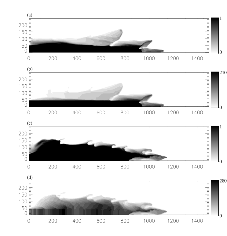
Figure 2: Plots (a) and (b) show the distribution of the jet tracer variable and $|\@vec{u}|$ for simulation C respectively. Plots (c) and (d) show the same quantities for simulation G. Plots (a) and (c) use a linear scale and a value of 1 indicates pure jet gas. Plots (b) and (d) also use a linear scale and are in units of km s^-1

Model	${\cal F}_{\rm H_{2}}$	${\cal F}_{\rm total}$	$\gamma$
A	0.21	0.58	2.42
B	0.20	0.55	2.93
C	0.08	0.36	2.37
D	0.07	0.36	2.08
E	0.07	0.36	1.81
F	0.09	0.33	2.31
G	0.10	0.38	2.98
G1	0.10	0.39	2.02
G2	0.10	0.39	3.75
H	0.06	0.16	1.58
I	0.08	0.21	2.44

Table 2: The proportion of momentum on the grid residing in ambient molecules (${\cal F}_{\rm H_{2}}$) and in all ambient gas (${\cal F}_{\rm total}$) at $t=300$ yrs. Also given is the value of $\gamma$, the power-law index for the mass-velocity relationship

3.2 The mass-velocity relationship

We do find a power-law relationship between mass of molecular gas and velocity. If we write

$$m(v)\propto v^{-\gamma}$$ (13)

then we find that $\gamma$ lies between 1.58 and 3.75 and that $\gamma$ tends to increase with time, in agreement with Smith et al. (smith (1997)). Table 2 shows the values of $\gamma$ at $t=300$ yrs for all the models. These values are consistent with observations (e.g. Davis et al. gam_obs (1998)), and also with the analytical model presented in the appendix of Smith et al. (smith (1997)) for the variations of mass with velocity. However, it is important to emphasise that what is actually observed is a variation in CO line intensity with velocity. CO line intensity is directly proportional to mass, in the relevant velocity channel, providing we are in the optically thin regime and the temperature of the gas is higher than the excitation temperature of the line (see, e.g.  McKee et al. mckee (1982)). Note that Smith et al. (smith (1997)) incorrectly state that the channel line brightness scales with $v^{2}\,dm(v)$. Fig. 3 shows a sample plot of the molecular mass versus velocity for the jet moving at an angle of $60^{\circ}$ to the plane of the sky. We do not see the jet contribution in the velocity range chosen here.

Figure 3: Plot of the relationship between the molecular mass and velocity for simulation G at $t=300$ yrs assuming the jet moves at an angle of $60^{\circ}$ to the plane of the sky. Note how a power-law (dashed line) fits the data quite well

The molecular fraction in the jet has a marked influence on the value of $\gamma$ predicted by these models as we can see by comparing the results for simulations G and G2. In fact, $\gamma$ increases with decreasing molecular abundance in the jet. This is due to the reduction in strength of the high velocity jet component.

It appears that $\gamma$ does not depend in a systematic way on the amplitude of the velocity variations. Note also that the introduction of a wide shear layer dramatically reduces $\gamma$. This is due to the fact that more gas is ejected out of the jet beam (because of the more strongly paraboloid shape of the internal working surfaces) and this accelerates the cocoon gas, leading to a stronger high velocity component. In addition, a wide shear layer causes the bow shock to be more blunt. It can be seen from the analytic model of Smith et al. (smith (1997)) that this also leads to a lower value of $\gamma$. It is interesting to speculate that lower values of gamma, which may be more common in molecular outflows from lower luminosity sources (see Davis et al. gam_obs (1998)) could result from such flows having a higher molecular fraction in their jets and perhaps a wide shear layer.

The behaviour of $\gamma$ with viewing angle is the same as that noted by Smith et al. (smith (1997)). The actual values of $\gamma$ obtained by these authors are somewhat lower than those obtained here. However, since our initial conditions are so different, and since $\gamma$ is dependent on the shape of the bow shock, this discrepancy is not disturbing.

3.3 H₂ proper motions and emissions

We measured the apparent motion of the emission from the internal working surfaces. Near the axis of the jet this emission moves with the average jet speed (i.e. $v_{0}$), as would be expected from momentum balance arguments. However, there are knots of emission arising from the bow shock itself and these move much more slowly ($\sim$5–15% of the average jet speed) with the faster moving knots being closer to the apex of the bow. This is in agreement with the observations of Micono et al. (micono (1998)).

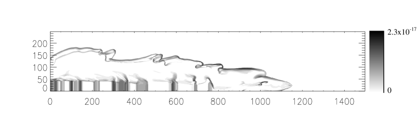
Figure 4: Log-scale plot of the distribution of emission from the S(1)1–0 2.12$\mu$ line of H₂ for simulation G after 300 yrs. The scale is in units of erg cm^-3 s^-1

Fig. 4 shows the emission from the S(1)1–0 line of H₂ for model G. There is little emission from the cocoon since the cocoon gas has been strongly shocked in the jet shock and so is mostly atomic. We can also see that the emission becomes more intense as we move away from the apex of the bow shock, as reported by many authors (e.g. Eislöffel et al. eisloffel (1994)). It is also clear that the internal working surfaces in the jet are giving rise to emission in this line. We can see that the emission begins to die away as we move away from the jet source. This is in agreement with observations of, for example, HH 46/47 (Eislöffel et al. eisloffel (1994)) where the emission from the knots appears close to the jet source and then fades away.

This decrease in emission happens for two reasons. The first is that the shocks in the jet become weaker as they move away from the source simply because the velocity variations, which give rise to the shocks in the first place, are smoothed out by the shocks (see, for example Whitham (Whitham (1974)). In addition, the mass flux through an individual shock decreases with time due to the divergent nature of the flow ahead of each internal working surface. This means that the emission will decrease because there is less gas being heated by the shock.

3.4 The ‘Hubble law’

We have found that the so-called ‘Hubble law’ (e.g. Lada & Fich LF (1996)) is reproduced in these simulations. Fig. 5 shows a position velocity diagram calculated from simulation G assuming that the jet makes an angle of $60^{\circ}$ to the plane of the sky. This diagram is based on the mass of H₂ rather than intensity of CO emission. There is a gradual, virtually monotonic, rise in the maximum velocity. It is also worth noting that near the apex of the bow shock the rise in the maximum velocity present becomes steeper. These properties are related to the shape of the bow shock as gas near the apex of the shock is moving away from the jet axis at higher speed than that far from the apex.

As a very basic model of this, suppose we represent the contact discontinuity between the post-shock jet and ambient gas to be an impermeable body moving with velocity $v$ through a fluid whose streamlines will follow the surface of the body. See Fig. 6 for a schematic diagram of the system. Let this surface be described by the equation

$$z=a-r^{s}$$ (14)

where $s\geq 2$ and $a$ is the position of the apex of the bow shock on the $z$ axis (see, e.g., Smith et al. smith (1997)). Since the contact discontinuity is a streamline of the flow we get that the ratio of the $z$-component to the $r$-component of the velocity is simply

$${\cal R}\equiv\frac{-v_{z}}{v_{r}}=s\left[a-z\right]^{\frac{s-1}{s}}$$ (15)

Note that this is the negative of the slope of the bow shock. This is because of our choice of the bow shock pointing to the right, and hence the $z$ component of the velocity will be negative. If we assume the post-shock velocity to be $v_{1}(z)$ (related to $v$ by the shock jump conditions), it is simple to show that

$$v_{r}(z)=\frac{v_{1}}{\sqrt{1+{\cal R}^{2}}}$$ (16)

Finally, after some simple algebra, we can write down the velocity along the line of sight as a function of $z$ by

$$v_{\rm los}(z)=\frac{v_{1}}{\sqrt{1+{\cal R}^{2}}}\left\{\cos\alpha+\cal{R}\sin\alpha\right\}$$ (17)

where $\alpha$ is the angle the bow shock makes to the plane of the sky. In fact we can write down $v_{1}(z)$ if we assume that the bow shock is a strong shock everywhere, thus yielding a compression ratio of 4 (from the shock conditions). It is easy to derive that

$$v_{1}(z)=v\cos\left(\arctan({\cal R})\right)\sqrt{\frac{1}{16}+{\cal R}^{2}}$$ (18)

This formula yields a shape for the position-velocity diagram which suggests the Hubble-law and is similar to diagrams generated from these simulations assuming that the flow is in the plane of the sky. This indicates that the ‘Hubble-law’ effect is, at least partly, an artifact of the geometry of the bow shock.

Figure 5: Contour plot of the position-velocity diagram (of mass rather than emission) for simulation G after 300 yrs assuming the jet moves at an angle of $60^{\circ}$ to the plane of the sky. Note the gradual rise of the maximum velocity as we move away from the source. The contours are logarithmic running from $3\times 10^{21}$ to $3\times 10^{25}$ g. The contribution from the jet is removed from this diagram to make the effect clearer

Figure 6: Schematic diagram of the setup used to derive the Hubble law for position-velocity diagrams. The fluid motion is shown by vectors. After contact with the bow shock, the fluid is assumed to flow along the contact discontinuity with a smaller, but constant, velocity. See text

3.5 Entrainment

As is clear from Fig. 2 there is not much extra entrainment of ambient gas resulting from the velocity variations. If the velocity variations were to involve the jet ‘switching off’ for a time comparable to the sound crossing time of the cocoon then we would expect ambient gas to move toward the jet axis and probably be driven into the cocoon when the jet switches on again. This does not happen in these simulations where the maximum period of the variations is 50 yrs and the amplitude is at most 60% of the jet velocity. However, there is a small amount of acceleration of molecular gas at the left-hand boundary of the grid. This effect is quite small, but may grow over time. It is also possible, however, that this effect is due simply to the reflecting boundary conditions.

These simulations show very little mixing between jet and ambient gas except very close to the apex of the bow shock. This means that the high velocity component of CO outflows often observed along the main lobe axis (Bachiller bachiller (1996)) is difficult to explain without invoking the presence of CO gas in the jet beam itself just after collimation.

4 Conclusions

It is now generally agreed that low velocity molecular outflows represent ambient gas that is somehow accelerated by highly collimated and partly ionized jets, at least in the case of low and intermediate mass YSOs. Most of this acceleration is thought to be achieved at the head of the jet through the leading bow shock (the so-called prompt entrainment mechanism). In this paper we have examined through many axially symmetric simulations the efficiency of the prompt entrainment mechanism as a means of transferring momentum to ambient molecular gas without causing dissociation. It is found, as one would expect, that the fraction of jet momentum transferred to the ambient environment depends on the jet/ambient density ratio. More importantly, we see that cooling, which is particularly important at higher densities, decreases the fractional jet momentum that goes into ambient molecules. It would seem on the basis of the simulations presented here that both heavy and equal density (with respect to the environment) jets with radiative cooling have very low efficiencies at accelerating ambient molecules without causing dissociation. In part this is because cooled jets have more aerodynamic bow shocks than the corresponding adiabatic ones (i.e. they present a smaller cross sectional area to the ambient medium). The actual shape, however, of the bow shock also seems to to be important as the decrease in momentum transferred to the ambient medium seems to affect the acceleration of molecules more so than atoms/ions.

We have also tested whether pulsed jets are more efficient at transferring momentum to the ambient medium than the corresponding steady jet with the same average velocity. Somewhat surprisingly we found that even relatively large velocity variations do not give rise to significant changes in the amount of momentum being deposited in ambient gas. Fundamentally this is because in high Mach number jets, even with cooling, there is very little coupling between the jet’s cocoon and the “sheath” (i.e. the post-shock ambient gas). This lack of coupling is also the reason why turbulent entrainment is not significant in YSO jets.

Our simulations were also used to model the expected variation of mass with velocity in molecular flows. We found relatively large $\gamma$ values, i.e. mass should decline steeply with velocity, in line with observations. Interestingly we found that a wide shear layer and an increasing molecular component in the jet reduced $\gamma$. If, as one might expect, such conditions are common among outflows from low luminosity YSOs, this could explain their observed lower values for $\gamma$. Finally we have shown that the so-called Hubble Law for molecular outflows is almost certainly a local effect in the vicinity of a bow shock.

Appendix A Overcoming negative pressures

As noted in §2.1 it is common for conservative numerical codes to predict negative pressures under certain conditions. Flows giving rise to such problems are usually highly supersonic, and diverging. The difficulties occur because the ratio of internal to total energy goes like $\frac{1}{M^{2}}$, where $M$ is the Mach number of the flow. Therefore, in a highly supersonic flow, the fractional error required to predict a negative pressure is rather small. The introduction of energy losses exacerbates this problem. This is due to the fact that relatively weakly diverging flows, for example, can become supersonically diverging when the system is cooled because the sound speed is reduced.

Schemes which are second order accurate in space tend to produce more negative pressures than first order ones. This is because first order schemes dissipate strong features quickly so that strongly diverging flows rarely occur. It seems reasonable, then, to invoke a scheme which is first order in space whenever a negative pressure is produced as this will introduce extra dissipation. This extra dissipation may eliminate the negative pressure by moving some extra energy from neighbouring cells into the problem one. The scheme used by the code in this work can be summarised as follows:

$$\@vec{U}^{n+1}_{i}=\@vec{U}^{n}_{i}-\lambda\left[{}^{2}\@vec{F}^{n+\frac{1}{2}}_{i+\frac{1}{2}}-\,^{2}\@vec{F}^{n+\frac{1}{2}}_{i-\frac{1}{2}}\right]$$ (19)

where $\@vec{U}^{n}_{i}$ and ${}^{2}\@vec{F}^{n}_{i}$ are the state vector and second order flux calculated at $t=n\Delta t$ and $x=i\Delta x$ respectively, and $\lambda=\frac{\Delta t}{\Delta x}$. If this scheme produces a negative pressure at $t=n+1$ then simply apply Eq. 19 using the first order fluxes ${}^{1}\@vec{F}^{n+\frac{1}{2}}_{i\pm\frac{1}{2}}$ instead of the second order ones. Note that it is necessary to adjust the neighbouring cells also so that overall conservation is maintained.

While this fix does not work for all problems, it was found to be rather effective in the simulations presented here where very strong rarefactions are produced both at the edge of the jet at the $z=0$ boundary, and within the jet itself where the enforced velocity variations can cause problems. This fix can be implemented very easily by ensuring that the flux vectors around problem cells are stored. It has the advantage that it does not involve losing conservation of any of the physically conserved quantities. Reducing the scheme to first order in certain regions of the grid is not a significant problem because this happens around shocks anyway in order to maintain monotonicity.

- (1) Bachiller, R., 1996, ARA&A, 34, 111
- (2) Cabrit, S., Raga, A., Gueth, F. 1997, in Herbig-Haro Outflows and the Birth of Low Mass Stars, IAU Symposium No. 182, eds. B. Reipurth & C. Bertout, Kluwer Academic Publishers, 163
- (3) Chernin, L.M., Masson, C.R. 1995, ApJ 455, 182
- (4) Davis, C.J., Eislöffel, J. 1995, A&A 300, 851
- (5) Davis, C.J., Moriarty-Schieven, G., Eislöffel, J., Hoare, M.G., Ray, T.P., 1998, ApJ 115, 1118
- (6) Dgani, R., van Buren, D., and Noriega-Crespo, A. 1996, ApJ 461, 927
- (7) Dove, J.E., Mandy, M.E. 1986, ApJ 311, L93
- (8) Downes, T.P. 1996, PhD Thesis (University of Dublin, Ireland)
- (9) Downes, T.P., Ray, T.P. 1998, A&A 331, 1130
- (10) Eislöffel, J., Davis, C.J., Ray, T.P., Mundt, R., 1994, ApJ 422, L91
- (11) Falle, S.A.E.G. 1991, MNRAS 250, 581
- (12) Falle, S.A.E.G., Raga, A.C. 1995, MNRAS 272, 785
- (13) Lada, C.J., Fich, M. 1996, ApJ 459, 638
- (14) Lepp, S., Shull, M.J. 1983, ApJ 270, 578
- (15) McKee, C.F., Storey, J.W.V., Watson, D.M., Green, S. 1982, A&A 113, 285
- (16) Micono, M., Davis, C.J., Ray, T.P., Eislöffel, J., Shetrone, M.D., 1998, ApJ, 494, L227
- (17) Padman, R., Bence, S., Richer, J. 1997, in Herbig-Haro Outflows and the Birth of Low Mass Stars, IAU Symposium No. 182, eds. B. Reipurth & C. Bertout, Kluwer Academic Publishers, 123
- (18) Raga, A.C., Cantó, J., Calvet, N., Rodríguez, L.F., Torrelles, J. 1993, A&A 276, 539
- (19) Smith, M.D., Suttner, G., Yorke, H.W. 1997 A&A 323, 223
- (20) Sutherland, R.S., Dopita, M.A. 1993, ApJS 88, 253
- (21) Suttner, G., Smith, M.D., Yorke, H.W., Zinnecker, H. 1997, A&A 318, 595
- (22) van Leer, B. 1977, J. Comp. Phys. 23, 276
- (23) Whitham, G.B. 1974, in Linear and Nonlinear Waves, John Wiley & Sons, 50.