HST Luminosity Functions of the Globular Clusters M10, M22, and M55. A comparison with other clusters.

Abstract

From a combination of deep Hubble Space Telescope $V$ and $I$ images with groundbased images in the same bands, we have obtained color–magnitude diagrams of M10, M22, and M55, extending from just above the hydrogen burning limit to the tip of the red giant branch, down to the white dwarf cooling sequence. We have used the color-magnitude arrays to extract main sequence luminosity functions (LFs) from the turnoff to $m\sim 0.13m_{\odot}$. The LFs of M10 is significantly steeper than that for the other two clusters. The difference cannot be due to a difference in metallicity. A comparison with the LFs from Piotto, Cool, and King (1997), shows a large spread in the LF slopes. This spread is also present in the local mass functions (MFs) obtained from the observed LFs using different theoretical mass–luminosity relations. The dispersion in the MF slopes remains also after removing the mass segregation effects by using multimass King-Michie models. The globular cluster MF slopes are also flatter than the MF slope of the field stars and of the Galactic clusters in the same mass interval. We interpret the MF slope dispersion and the MF flatness as an evidence of dynamical evolution which makes the present day globular cluster stellar MFs different from the intial MFs. The slopes of the present day MFs exclude that the low mass star can be dynamically relevant for the Galactic globular clusters.

1 Introduction

The Hubble Space Telescope (HST) allows the derivation of color magnitude diagrams (CMDs) of Galactic globular clusters (GCs) which extend to almost the faintest visible stars, just above the hydrogen-burning limit for the nearest clusters (King et al.  1998). These CMDs can be used to extract luminosity functions (LFs), and from them mass functions (MFs) which extend over almost the entire mass range of the luminous GC stars, from the turnoff (TO) down to the bottom of the main sequence ($0.1\leq m/m_{\odot}\leq 0.8$).

The GC MFs are important as they can provide important observational inputs in a variety of astrophysical problems, like the realistic dynamical modeling of individual clusters (King, Sosin, and Cool 1995, Sosin 1997), and the role of dynamical evolution in modifying the GC stellar content (Piotto, Cool, and King 1997, PCK). In principle, GC MFs also give information about the amount of mass contained in very-low-mass stars and brown dwarf stars in globulars, and, by extension, in the Galactic halo. The observed MFs are related to the GC initial MFs (IMFs): a basic input parameter for any GC and galaxy formation model.

Progress on these issues requires accurate photometry of main sequence (MS) stars. In many cases, the HST data alone cannot provide all the information. The brightest MS stars in the closest GCs are always badly saturated in deep WFPC2/HST frames, and often there are no short exposures in the same field, as we tend to use HST to measure the faintest objects. This lack of information might become a dangerous drawback when comparing the stellar LF of different clusters, as discussed in Cool, Piotto, and King (1996, CPK). In fact, the shape of the LF for stars fainter than $M_{V}\sim 8$ is dominated by the slope of the mass-luminosity relation (MLR) more than by the shape of the MF. Ground-based data might become of great importance in this respect.

Here we present the first deep HST CMDs and LFs for M10 (NGC 6254) and M55 (NGC 6809), and an independent determination of the CMD and the LF of M22 (NGC 6656). A CMD and a LF of M22 have already been presented by De Marchi and Paresce (1997), based on the same images. For all three clusters, the CMDs and LFs have been extended to the TO and above, by means of ground-based data. We compare the results for M22 with the LF of De Marchi and Paresce (1997), and then compare the LFs for the three clusters with each other. A comparison with the presently available HST LFs and MFs for intermediate and metal-poor clusters is also presented. This paper is a continuation and an extension of the paper by PCK.

A description of the observations and of the data analysis is presented in Section 2. The CMDs and LFs are presented in Sections 3 and 4. The MF is derived in Section 5. A comparison of the presently available LFs extended to the TO is shown in Section  6, and a discussion follows in Section 7.

Table 1: Data Set

Object	Telescope	Obs. date	Filter	Exp. time (s)
M22	HST	30-9-1995	F606W	1100
	”	”	F606W	1200$\times$3
	”	”	F814W	1100
	”	”	F814W	1200$\times$3
	DUTCH	15-4-1997	V	45
	”	”	V	1500
	”	”	I	45
	”	”	I	1500
M55	HST	4-11-1995	F606W	1100
	”	”	F606W	1200$\times$5
	”	”	F814W	1100
	”	”	F814W	1200$\times$5
	DUTCH	15-4-1997	V	45
	”	”	V	1500
	”	”	I	45
	”	”	I	1500
M10	HST	10-10-1995	F606W	1100
	”	”	F606W	1200$\times$9
	”	”	F814W	1100
	”	”	F814W	1200$\times$9
	JKT	30-5-1997	V	15
	”	”	V	45
	”	”	V	1500
	”	”	I	15
	”	”	I	45
	”	”	I	1500

2 Observations and Analysis

The data presented in this paper consist of a set of WFPC2 images and a set of ground-based frames covering approximately the same field for the three GCs M10, M22, and M55.

The WFPC2 data have been taken from the ST-ECF HST archive and were obtained with the F606W and F814W filters during Cycle 5. The observation dates and the exposure times are given in Table 1. The fields are located at about 3.0 arcmin (for M10), 4.5 arcmin (for M22), and 3.0 arcmin (for M55) from the cluster centers. The HST archive data did not include short exposures. This fact made impossible the photometry of any stars brighter than V$\sim 19.0$, because of the CCD saturation problems. This means that the CMDs and the LFs from the HST photometry are truncated at about two magnitudes below the TO.

In order to extend both the CMDs and the LFs to the TO and above, we collected a set of short-exposure images with three 1-m size telescopes. For M22 we used the 0.9m Dutch telescope at ESO (La Silla), the 1.54m Danish telescope at ESO for M55, and the 1.0m Jacobus Kapteyn Telescope (JKT) at La Palma (Islas Canarias) for M10 (cf. Table 1 for the observation dates and the exposure times). The seeing conditions were exceptionally good at the JKT (0.7 arcsec FWHM), while the average seeing conditions for the ESO images were 1.2 arcsec FWHM. The ground-based images for M10 and M22 were collected in photometric conditions, while the M55 data come from a non-photometric night.

2.1 HST data reduction

All HST observations were pre-processed through the standard HST pipeline with the most up-to-date reference files. Following Silbermann et al.  (1996), we have masked out the vignetted pixels, saturated and bad pixels and columns using a vignetting mask created by P.B. Stetson together with the appropriate data quality file for each frame. We have also multiplied each frame by a pixel area map (also provided by P.B. Stetson) in order to correct for the geometric distortion (Silbermann et al.  1996).

The photometric reduction was carried out using the
DAOPHOT II/ALLFRAME package (Stetson 1987, 1994). A preliminary photometry was carried out in order to construct an approximate list of stars for each single frame. This list was used to accurately match the different frames. With the correct coordinate transformations among the frames, we obtained a single image, combining all the frames, regardless of the filter. In this way we could eliminate all the cosmic rays and obtain the highest signal/noise image for star finding. We ran the DAOPHOT/FIND routine on the stacked image and performed PSF-fitting photometry in order to obtain the deepest list of stellar objects free from spurious detections. Finally, this list was given as input to ALLFRAME, for the simultaneous PSF-fitting photometry of all the individual frames. The PSFs we used were the WFPC2 model PSFs extracted by P.B. Stetson (1995) from a large set of uncrowded and unsaturated images.

We transformed the F606W and F814W instrumental magnitudes into the standard $V$ and $I$ systems using Eq. (8) of Holtzman et al.  (1995) and the coefficients in their Table 7.

Note that the CMDs of M10, M22, and M55 presented in the following come from the combination of the photometry in the three WF chips. The LFs have been obtained from chip WF2 for M10, from WF3 for M22, and WF4 for M55. These fields contain the largest number of unsaturated stars and the smallest number of saturated pixels. In view of the small error bars of the LFs presented in Section 4, we considered it not worth the large cpu time that would have been required to run crowding experiments for every chip.

2.2 Ground-based data reduction

Image pre-processing (bias subtraction and flatfielding) was carried out using standard IRAF routines. The stellar photometry has been obtained using DAOPHOT II/ALLFRAME as described above on all the images (including the short exposures) simultaneously. We constructed the model PSF for each image using typically $\sim$ 120 stars.

Since some of the ground-based images have been collected on non-photometric nights, the calibration of the instrumental magnitudes was performed by comparison with the stars in the overlapping HST fields. We first adopted the color term obtained for the same telescopes during the previous nights in the same run (Rosenberg et al.  1999). The zero points have been calculated by comparing all the non-saturated stars in the WFPC2 chips that were also measured in the ground-based images. The uncertainties in the $V$ zero points are 0.004, 0.035, and 0.015 magnitudes (the errors refer to the errors on the mean differences) for M10, M22, and M55, respectively. The errors in the $(V-I)$ colors are 0.006, 0.055, and 0.025, respectively. The zero point uncertainties for M22 are noticeably larger than for the other two clusters. This fact is due to the smaller overlap in magnitude between the ground-based and the HST photometries, as can be seen in Fig. 2. The calibration of the M22 and M55 CMDs has been further checked by comparing these diagrams with other independently calibrated $V$ vs. $(V-I)$ ground-based CMDs kindly provided by Alfred Rosenberg (Rosenberg et al.  1999). The two sets of data are consistent within the uncertainties given above.

Shorter-exposure HST images (or longer-exposure ground-based frames) are desirable for a smoother overlap of the two data sets. Note that this problem does not affect the LF presented in Section 4. Indeed, a zero point error of a few hundreds of a magnitude is perfectly acceptable for a LF with magnitude bins of 0.5 mag.

2.3 Artificial star tests

Particular attention was devoted to estimating the completeness of our samples. The completeness corrections have been determined by standard artificial-star experiments on both the HST and ground-based data. For each cluster, we performed ten independent experiments for the HST images and five for the ground-based ones. In order to optimize the cpu time, in our experiments we tried to add the largest possible number of artificial stars in a single test, without artificially increasing the crowding of the original field. The artificial stars have been added in a spatial grid such that the separation of the centers in each star pair was two PSF radii plus one pixel. The position of each star is fixed within the grid. However, the grid was randomly moved on the frame in each different experiment. We verified that in this way we were not creating over-crowding by running an experiment with half the number of artificial stars. The finding algorithm adopted to identify and measure the artificial stars was the same used for the photometry of the original images. The artificial stars were added on each single V and I frame. For each artificial star test, the frame to frame coordinate transformations (as calculated from the original photometry) have been used to ensure that the artificial stars were added exactly in the same position in each frame. We started by adding stars in one V frame at random magnitudes; the corresponding I magnitude for each star was obtained using the fiducial line of the instrumental CMD. Finally, in each band, we scaled the magnitudes according to the frame to frame magnitude offset as calculated from the original photometry. The frames obtained in this way were stacked together in order to perform star finding and obtain the most complete star list. The latter was used to reduce the single frames simultaneously with ALLFRAME, following all the steps and using the same parameters as on the original images.

In order to take into account the effect of the migration of stars toward brighter magnitudes in the LF (Stetson & Harris 1988), we corrected for completeness using the matrix method described in Drukier et al.  (1988).

In the LFs presented here, we include only points for which the completeness figures were 50% or higher, so that none of the counts have been corrected by more than a factor of 2.

A comparison between the added magnitudes and the measured magnitudes allows also a realistic estimate of the photometric error $\sigma_{{\rm pho}}$ (defined as the standard deviation of the differences between the magnitudes added and those found) as a function of magnitude. We use this information in different places in what follows.

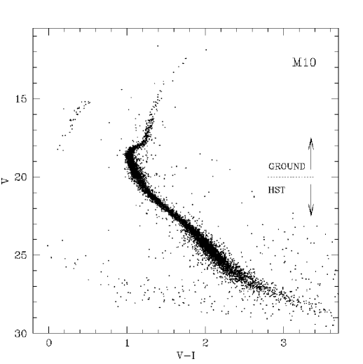
Figure 1: Composite CMD for 6986 stars in M10. The ground-based data are from the JKT telescope.

3 The color-magnitude diagrams

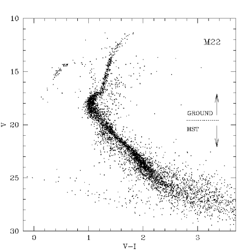
Figure 2: Composite CMD of 5385 stars in M22. The ground-based data are from the ESO-Dutch telescope. For the HST data only the stars in the WF2 field are shown.

The CMDs derived from the photometry discussed in the previous Section are presented in Figs. 1, 2, and 3. The upper part of the CMDs comes from the ground-based data, while the lower part is from the three WF cameras of the WFPC2. In the case of M22, the CMD for magnitudes fainter than V=19.8 comes from the WF2 only: the differential reddening of this cluster (Peterson and Cudworth 1994) makes the sequence much broader than expected from the photometric errors. The MS of M22 from the three WF cameras is shown in Fig. 4. In Table 2 the dispersion $\sigma_{MS}$ (defined as the sigma of the best fitting gaussian) of the MS (after the removal of the field star contamination as described in Section 4) is compared with the expected photometric error $\sigma_{(V-I)}$. The latter have been estimated from the artificial star tests (cf. Section 2.3), in one magnitude bins, in the interval $20<V<26$. The resulting average differential reddening in the 3 WF fields is $\langle\sigma_{{\rm red}}\rangle=\big{\langle}\sqrt{\sigma_{{\rm MS}}^{2}-\sigma_{(V-I)}^{2}}\big{\rangle}=0.05$ magnitudes. This value must be considered as an upper limit for the differential reddening in this region.

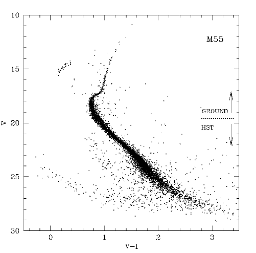
Figure 3: Composite CMD of 8121 stars in M55. The ground-based data are from the ESO-Danish telescope.

Table 2:

$$\begin{array}[]{llll}\hline\cr\vskip 3.0pt plus 1.0pt minus 1.0pt\cr V&\sigma_{MS}&\sigma_{(V-I)}&\sigma_{red}\\ \vskip 3.0pt plus 1.0pt minus 1.0pt\cr\hline\cr\vskip 3.0pt plus 1.0pt minus 1.0pt\cr 20.5&0.068&0.036&0.058\\ 21.5&0.069&0.045&0.052\\ 22.5&0.072&0.052&0.048\\ 23.5&0.081&0.071&0.039\\ 24.5&0.093&0.079&0.049\\ 25.5&0.100&0.086&0.051\\ \vskip 3.0pt plus 1.0pt minus 1.0pt\cr\hline\cr\end{array}$$

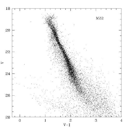
Figure 4: CMD of 13359 stars from the three WF fields of M22. The large dispersion of the MS is interpreted in terms of a differential reddening of $\sim 0.05$ magnitudes in $(V-I)$.

The ground-based and the HST fields are partially overlapping, with the ground-based images always covering a larger portion of the cluster. A detailed discussion of these CMDs will appear elsewhere. Here it suffice to note that we measured stars from the tip of the giant brach to a limiting magnitude $V\sim 28$. A white dwarf cooling sequence is clearly seen in all diagrams (but it will be discussed elsewhere). For the first time, we have a complete picture of a simple stellar population about 15 Gyr after its birth, from close to the hydrogen-burning limit to the final stages of its evolution along the white dwarf sequence. These diagrams can be used for a fine tuning of the stellar evolution and population synthesis models (Brocato et al.  1996).

Contamination by foreground/background stars is small for M10, as expected from its galactic latitute ($b=23^{\circ}$), though a few background stars (likely from the outskirts of the Galactic bulge) are present. Despite the fact that M55 has the same latitude as M10, a significantly larger fraction of field stars is visible in the CMD of Fig. 3. Some of these stars are likely bulge members, but the prominent sequence blueward of the MS of M55 must be associated with the MS and TO of the stars in the Sagittarius dwarf spheroidal galaxy (Mateo et al.  1996, Fahlman et al.  1996). M22 is the most contaminated cluster. Both Galactic disk and Galactic bulge stars are clearly seen in the CMDs of Figs. 2 and 4.

Deep CMDs also contain information on the low-mass content of the clusters. This information can be extracted from our data only after we have a reliable transformation from luminosities to masses. Unfortunately, such a transformation remains uncertain for low-metallicity, low-mass stars. Almost nothing is known from the empirical point of view, and different calculations of stellar models yield different masses, particularly for the lowest-mass stars (King et al.  1998), and different overall trends (slopes) for the mass-luminosity relations (MLRs).

Figure 5: Comparison between the observed CMD of M10 and the models by the Lyon group (left panel), and the Teramo group (right panel) for [M/H] $=-1.3$ (solid line) and [M/H] $=-1.5$ (dashed line). The open circles represent the MS ridgeline.

Figure 6: Comparison between the observed CMD of M22 and the models by the Lyon group (left panel), and the Teramo group (right panel) for [M/H] $=-1.5$ (dashed line) and [M/H] $=-2.0$ (solid line). The open circles represent the MS ridgeline.

Figure 7: Comparison between the observed CMD of M55 and the models by the Lyon group (left panel), and the Teramo group (right panel) for [M/H] $=-1.5$ (dashed line) and [M/H] $=-2.0$ (solid line). The open circles represent the MS ridgeline.

As already found for NGC 6397 (King et al.  1998) and the other three metal-poor clusters studied by PCK (cf. their Fig. 3), among the existing models we find that those by the group in Lyon (Baraffe et al.  1997) and by the group in Teramo (Cassisi et al.  1998, in preparation) best reproduce the observed sequences of M10, M22, and M55. [Note that Cassisi et al.’s (1998) models below $0.5m_{\odot}$ ($M_{V}\sim 8.1$) are the same models as in Alexander et al.  (1997).] The level of agreement between the models and the observed data can be fully appreciated in Figs. 5, 6, and 7. In these figures the open circles represent the MS ridgeline, obtained by using a mode-finding algorithm and a kappa-sigma iteration in order to minimize the field star contamination. The dotted line represents the $V$ magnitude limit of the LFs presented in the following Section 4; the data below this magnitude limit are not used in the present paper. The dashed line shows the isochrone corresponding to the metallicity which best matches the Zinn and West (1984) [Fe/H] (iron) content, scaled to the appropriate metallicity [M/H] assuming [O/Fe]=0.35 (Ryan and Norris 1991), and using the relation by Salaris, Chieffi, and Straniero (1993). According to Table 3, we used the models for [M/H] $=-1.5$ for M22 and M55, and the models for [M/H] $=-1.3$ for M10. For comparison reasons, in Figs.5, 6, and 7 we show also the isochrones which best match the Zinn and West (1984) metallicity assuming a solar ratio for the alpha elements (solid line). The distance modulus and reddening have been left as free parameters. The resulting values of $(m-M)_{V}$ are in very good agreement with the values in the literature (cf. Djorgovski 1993). This is also true for the $E(V-I)$ resulting from the fit of the Lyon group models. The models from the Teramo group result systematically redder by about 0.06 magnitudes in $(V-I)$ than the isochrones from Baraffe et al.  (1997), and the resulting reddening is marginally consistent with the reddening in the literature. In the LF comparison discussed in Section 4, we have adopted the distance moduli and reddenings used in the fit of the Baraffe et al.  models and listed in Table 3.

We want to briefly comment on the comparisons in Figs.5, 6, and 7, leaving a more complete discussion to a future paper specific to the CMDs. There is an overall agreement between the models and the observed sequences. With the adopted distance moduli, both sets of models reproduce the characteristic bends of the MS, and at the correct magnitudes. The MSs of M22 and M55 seem to be better reproduced by the models, while the discrepancies seems to be more significant for M10. The deviations close to the TO might be due to the age of the adopted isochrones (the only ones available to us), which is 10 Gyr for the Lyon models and 14 Gyr for the Teramo ones. The isochrones seem to deviate more and more in color in the lowest part of the CMD. We can exclude that this is due to any internal errors in our photometry. The artificial-star experiments show that the average deviation in color due to photometric errors is less than 0.03 magnitudes at the faintest limit of the photometry. The residual differences might arise both from errors in the calibration from the HST to the standard $(V,I)$ system and to errors in the transformation from the theoretical to observational plane, very uncertain for these cool stars (Alexander et al.  1997).

Table 3: Adopted Parameters

Object	model	$(m-M)_{V}$	E(B-V)	[M/H]
M10	Baraffe et al.	14.20	0.29	-1.3
	Cassisi et al.	14.25	0.23	-1.3
M22	Baraffe et al.	13.70	0.37	-1.5
	Cassisi et al.	13.71	0.31	-1.54
M55	Baraffe et al.	13.90	0.14	-1.5
	Cassisi et al.	14.15	0.10	-1.54

4 The luminosity functions

The principal objective of the present work is to measure main-sequence luminosity functions. To this end, we followed the same procedure outlined in CPK and PCK. We started by locating the ridge line of the MS using a kappa-sigma clipping algorithm both on the ground-based and on the HST data. The mode of the $(V-I)$ distribution was calculated in bins 0.25 mag wide in $V$. The next step was to subtract the MS ridge-line color from the measured color of each star, in order to produce a CMD with a straightened MS. Two lines, to the left and right of the straightened sequence, were then used to define an envelope around the MS. A range of $\pm 3\sigma$ (where $\sigma$ is the standard deviation of the photometric errors obtained from the artificial-star experiments) was used in order to encompass nearly all the MS stars. Stars within this envelope were binned in 0.5 mag intervals in order to produce a preliminary LF. These LFs must be corrected for field-star contamination. The field-star density was estimated by taking the average of the star counts in strips of width $6\sigma$ outside each side of the MS envelope. In M10 and M55 the correction for field stars was always less than 10%.

The case of M22 is more complicated. The field-star contamination is below 10% only in the magnitude interval $21.5<V<26$. At $V=26.25$ the contamination is already 15%. At fainter magnitudes, it becomes rather uncertain because of the spread of the MS due to the photometric errors. We think that below $V=26.5$ ($I=23.8$) it is not possible to estimate the field star contamination reliably with the present data for M22. In the magnitude interval $19.5<V<21.0$ the red giant branch of the bulge crosses the MS of M22, creating additional problems for the estimate of the field-star contamination. In this magnitude interval we estimated the amount of contamination using the counts obtained running the code by Ratnatunga and Bahcall (1985), normalized to the number of field stars we found in the box defined by $21.5<V<20.0$ and $1.0<(V-I)<1.5$ in the CMD of Fig. 2. For this cluster, a more reliable LF can be obtained only with second-epoch HST observations of the same field analyzed in this paper, as was done by King et al.  (1998) for NGC 6397.

Both the $V$ and $I$ LFs for the three clusters are shown in Figs. 8, 9, and 10 and listed in Tables 4, 5, and 6. Col. 1 gives the $V$ magnitudes, Col. 2 gives the field-star corrected LF, and Col. 3 lists the corrected (for both field star contamination and incompleteness) counts. The same figures for the $I$ LFs are in Cols. 4–6. The LFs listed in Tables 4–6 are from the HST photometry up to the brightest magnitude bin of the HST data; for brighter magnitudes Tables 4–6 list the ground-based LFs scaled to the area of one WF CCD.

Figure 8: The $V$ (lower panel) and $I$ (upper panel) ground-based (open circles) and HST (filled circles) LFs of M10 from the CMD of Fig. 1. The ground-based LFs have been scaled to the HST area. The arrows indicate the TO position. The error bars are plotted only when they exceed the symbol size.

Figure 9: The $V$ (lower panel) and $I$ (upper panel) ground-based (open circles) and HST (filled circles) LFs of M22 from the CMD of Fig. 2. The ground-based LFs have been scaled to the HST area. The arrows indicate the TO position. The error bars are plotted only when they exceed the symbol size. The open triangles show the LF obtained by De Marchi and Paresce (1997) from the same HST data.

Figure 10: The $V$ (lower panel) and $I$ (upper panel) ground-based and HST (filled circles) LFs of M55 from the CMD of Fig. 3. The ground-based LFs are from Zaggia et al.  (1997, filled triangles) and Mandushev et al.  (1996, open circles). The LF from Zaggia et al.  have been normalized to the HST area, while the Mandushev et al.  LF has been scaled to the total counts in the common magnitude range. The arrows indicate the TO position. The error bars are plotted only when exceeding the symbol size.

The ground-based LFs in Figs. 8 and 9 (open circles) have been obtained from the CMDs of Figs. 1 and 2, respectively. As the ground-based and HST LFs (filled circles) have been obtained at the same distance from the cluster center, they have been normalized by scaling the ground-based counts to the area of the HST field. In Fig. 10 we compare the HST LF of M55 with the LFs from Zaggia et al.  (1997) and from Mandushev et al.  (1996). Note that the data of Zaggia et al.  refer to the same radial interval as the HST data, while the field of Mandushev et al.  is located in an outer region (at 6.8 arcmin from the cluster center). In this case, the LF has been normalized to the others by using the total star counts in the common magnitude interval. Note the good agreement among the three LFs in the common region. The LF of Mandushev is slightly steeper than the HST LF, particularly at the lower end; this might be due to a mass-segregation effect. In Fig. 9 the open triangles show the LF obtained by De Marchi and Paresce (1997) from the same HST data. Despite the fact that the photometry has been obtained in a completely independent way, and using rather different reduction procedures, it is comfortable to see that there is perfect agreement between the two LFs down to $I=23.25$, where the completeness is only 56% (cf. Table 5). We have already commented how, below $I\sim 23.5$, the incompleteness and, most importantly, the difficulties in the field-star contamination estimates make the LF rather uncertain, and we prefer to avoid presenting data that are too uncertain.

As was discussed in Section 1, all three clusters have comparable metallicities (within $\sim 0.3$ dex). This fact allows to compare directly their LFs, without having to pass through the uncertain MLRs. Similarities or differences among the LFs of the three clusters reflect directly similarities or differences in their MFs. In addition, the HST fields where the LF was measured for M10, M22, and M55 are all located very close to the half-mass radius ($r_{{\rm obs}}/r_{{\rm h}}$=1.1 for M55, $r_{{\rm obs}}/r_{{\rm h}}$=1.4 for M10, and $r_{{\rm obs}}/r_{{\rm h}}$=1.8 for M22). This is a particularly fortunate case, as Vesperini and Heggie (1997), among others, have shown that the LF observed close to the half-mass radius in a King model (i.e., not collapsed) cluster, is close to the global (present day) LF. In other words, as a first approximation, our LFs do not need any mass-segregation correction.

Table 4: M10 Luminosity Function

$V$	$N$	$N_{corr}$	$I$	$N$	$N_{corr}$
18.25	9	11	16.75	4	4
18.75	16	20	17.25	6	9
19.25	21	27	17.75	11	20
19.75	25	32	18.25	16	30
20.25	53	46	18.75	41	34
20.75	72	68	19.25	75	64
21.25	87	94	19.75	98	98
21.75	89	78	20.25	115	115
22.25	79	68	20.75	101	99
22.75	108	110	21.25	149	157
23.25	116	124	21.75	179	202
23.75	163	187	22.25	222	255
24.25	188	220	22.75	250	323
24.75	203	260	23.25	180	243
25.25	175	230	23.75	141	195
25.75	126	167	24.25	104	150
26.25	102	161	24.75	46	86
26.75	55	75
27.25	45	80
27.75	19	34

Table 5: M22 Luminosity Function

$V$	$N$	$N_{corr}$	$I$	$N$	$N_{corr}$
15.25	6	6	13.94	5	5
15.75	5	5	14.46	5	5
16.25	8	8	14.99	7	7
16.75	10	10	15.54	8	8
17.25	29	29	16.17	22	22
17.75	40	48	16.69	44	36
18.25	51	65	17.16	65	51
18.75	59	83	17.63	81	58
19.25	76	82	18.25	105	104
19.75	89	89	18.75	127	128
20.25	120	106	19.25	119	130
20.75	111	108	19.75	123	145
21.25	141	137	20.25	144	175
21.75	149	144	20.75	197	264
22.25	185	195	21.25	292	395
22.75	215	249	21.75	272	427
23.25	244	295	22.25	237	397
23.75	245	301	22.75	189	325
24.25	197	276	23.25	140	251
24.75	164	243
25.25	125	181
25.75	121	226
26.25	77	146

Table 6: M55 Luminosity Function

V	N	$N_{corr}$	I	N	$N_{corr}$
19.75	89	94	18.75	96	120
20.25	93	100	19.25	109	120
20.75	89	107	19.75	109	127
21.25	95	101	20.25	135	148
21.75	96	98	20.75	142	162
22.25	132	142	21.25	189	235
22.75	151	173	21.75	255	330
23.25	201	240	22.25	285	378
23.75	256	341	22.75	224	321
24.25	229	274	23.25	158	242
24.75	166	247	23.75	108	175
25.25	115	149	24.25	73	140
25.75	99	150
26.25	57	83

The comparison is shown in Fig. 11 ($V$ LFs) and Fig. 12 ($I$ LFs). The adopted apparent distance moduli and reddenings are given in Table 3 (Baraffe et al.  rows). In the absence of a means of normalizing the three LFs to a global cluster parameter, arbitrary constants determine the vertical positioning of the individual LFs. We have chosen these constants exactly as described in PCK. Briefly, vertical shift of the M10, M22, and M55 LFs were made to bring them into alignment, according to a least-square algorithm, in the magnitude intervals $4.0<M_{{\rm V}}<6.0$ and $3.5<M_{{\rm I}}<5.5$. The overall trend of the LFs in Fig. 11 and Fig. 12 is similar, with a steep rise up to $M_{V}\sim 10$ ($M_{I}\sim 8.5$), followed by a drop to the limiting magnitude of the present investigation. Indeed, both the $V$ and $I$ LFs for M10 reach their maximum at magnitudes $\sim 0.5$ fainter than in M55 and M22. This is qualitatively consistent with the fact that M10 is slightly more metal rich than the other two clusters (D’Antona and Mazzitelli, 1995).

Figure 11: The $V$ LFs of M10, M22, and M55. The three LFs have been extended to the TO using the ground-based data. The horizontal bars indicate the normalization interval. The LFs of M10 is steeper than the other two. The difference in slope is significantly higher than what expected from the stellar structure models.

Figure 12: As in Fig. 11, but for the $I$ LFs. Again the LF of M10 is significantly steeper.

Despite the fact that the overall shape of the LF of M10 is similar to the others, a close inspection of Figs. 11 and 12 reveals that it is significantly steeper than the other two LFs. This difference can hardly be due to any internal dynamical evolution, if we consider that the three clusters have similar internal structures. Even if we did not fully trust the dynamical models (both King-Michie models and N-body simulations, Vesperini and Heggie 1997), which predict that our local LFs for M10, M22, and M55 closely resemble the global ones, it is noteworthy that the M10 field is at an intermediate position in terms of half-light radius $r_{h}$, between the M55 and the M22 fields. Therefore, the differences in LF slopes cannot be due to mass segregation.

5 The mass functions

Figure 13: The MFs of M10, M22, and M55 from the $I$ LFs and from different theoretical MLRs are compared. For reasons of clarity the MFs are arbitrarily shifted on the vertical axis.

Figure 14: Comparison of the MFs of M10, M22, and M55 from the $V$ and $I$ LFs and from the Teramo MLRs. For reasons of clarity the MFs are arbitrarily shifted on the vertical axis.

The LFs can be transformed into MFs using a MLR. As emphasized in Section 3, such transformations are still uncertain for low-mass, low-metallicity stars, and we must rely on the models almost entirely. It is somehow reassuring that not only at least two of the existing models are able to reproduce the observed diagrams, but also the distance moduli and reddenings that result from the fit are in agreement, within the errors, with the values in the literature. This does not mean that the models by the Lyon and the Teramo groups used in Section 3 are the correct ones. They are simply the best ones presently available, and we will use both of them to gather some information on the general shape of the MFs of M10, M15, and M22. The cautionary remarks on the absence of empirical MLR data should still be heeded. For the sake of comparison, and in order to give an idea of the possible range of uncertainty, we will also use the MLR of the Roma group (D’Antona and Mazzitelli 1995).

In Fig. 13 we compare the MFs derived from the $I$ LFs of M10, M22, and M55 from the TO down to $\sim 0.11m_{\odot}$. An arbitrary vertical shift is applied for reasons of clarity. The adopted distance moduli, reddenings, and metallicities for the MFs obtained using the Lyon and Teramo models are in Table 3. For the Roma model we adopted the values in Djorgovski (1993) and used the isochrone corresponding to 10 Gyr.

The MFs obtained using the Lyon and Teramo models track one other closely for $m<0.6m_{\odot}$. The small differences for higher masses might be due, at least in part, to the difference in the adopted ages. The MFs from the Roma models are systematically steeper, as already noted in PCK. Fig. 14 compares the MFs obtained from the $V$ and $I$ LFs, using the Teramo models. In all cases, the two MFs are very similar, despite the fact that the two LFs have been independently obtained. This result is also reassuring on the theoretical side, showing the internal consistency of the models.

In all cases, there is a hint of flattening at the low-mass end, but no sign of a drop-off.

As the transformation from the LF to the MF is the weakest part of the present analysis, we prefer not to comment further on the detailed structure of the MF. We note only that the slopes of the MFs below $0.5m_{\odot}$, using any existing MLRs, are shallower than the $x=1$ slope ($x=1.35$ for the Salpeter MF in this notation) for which the integration of the total mass down to $m=0$ would diverge.

6 Comparison with other clusters

Figure 15: The theoretical LFs from the Baraffe et al.  (1997) models for a power law MF with slope x=-0.3 and metallicities as shown in the labels are compared with the V LFs on M15, M30, M92, and NGC 6397. In the metallicity interval covered by the clusters in our sample, the theoretical LFs look quite similar.

It is interesting to compare the LFs in Fig. 11 and 12 with the LFs of other GCs with similar metallicity. The only other homogeneous set of $V$ and $I$ LFs extending from the TO to $m<0.15m_{\odot}$ has been collected by PCK for M15, M30, M92, and NGC 6397. In addition, Ferraro et al.  (1997) have published an $I$ LF for NGC 6752. There are two other clusters, which have a metallicity comparable to M22 and M10, and for which deep HST LFs have been published: $\omega$ Cen (Elson, Gilmore, and Santiago 1995) and M3 (Marconi et al.  1998). In both cases, saturation of the brightest stars does not allow to extend the LFs to the TO and we will omit them in the present comparison.

Figure 16: As in Fig. 17, but for the $I$ LFs. The $I$ LF of NGC 6397 is from King et al.  (1998). The LF of NGC 6752 is from Ferraro et al.  (1997). As in Fig. 17, note the spread in slope.

Figure 17: The $V$ and $I$ LFs of M10, M22, and M55 are compared with the LFs of all the clusters with [Fe/H]$<-1.6$ available in the literature. Only the LFs which extend to the TO are used. The LFs for M15, M30, M92, and NGC 6397 are from PCK The horizontal bars show the adopted normalization interval. Note the spread in slope of these LFs, significantly larger than expected from the error bars (cf. Fig. 11) and the metallicity differences (cf. Fig. 15).

As discussed in King et al.  (1995) and PCK, at the intermediate radius at which M15, M30, M92, and NGC 6397 were observed, their LFs are fortuitously close to the global ones, with differences that nowhere exceed a few tenths in the logarithm (PCK), with the local LFs being always steeper than the global ones. So, a comparison of these LFs with the LFs of M10, M22, and M55 should be only marginally affected by mass segregation effects. Unfortunately, no detailed dynamical model for NGC 6752 is available at the moment. We ran a multi-mass King-Michie model on this cluster (cf. Section 7). We find that the locally observed LFs of NGC 6752 is significantly flatter than the global one.

Figure 18: As in Fig. 16, but with a different normalization interval.

The metallicity of the three clusters presented in this paper is slightly higher than that of the clusters in PCK. We need to investigate the effect of this metallicity spread on the LFs. In Fig. 15 the theoretical LFs for a power law MF with a slope x=0.3 and three different metallicities are plotted together with the $V$ LFs of the four clusters in PCK used as reference. The three theoretical LFs are quite similar in the metallicity interval which span the entire metallicity range of the clusters discussed in the following.

Figs. 17 and 16 compare the $V$ and $I$ LFs of M10, M22, and M55 with the LFs of all the clusters with [Fe/H]$<-1.6$ available in the literature. Only the LFs which extend to the TO are used. The overall shape of the LFs is similar for the eight clusters, with a steep rise up to $M_{V}\sim 10$ ($M_{I}\sim 8.5-9.0$), followed by a drop to the limiting magnitude. As shown in Fig. 15 this shape is mainly due to the mass-luminosity relation (MLR) and not to the morphology of the MF (cf. also Section 5). Despite the fact that the general trend of these LFs is similar, their slope is different. These differences are much larger than expected from the error bars (Figs. 11 and 12) and from the cluster metallicity differences (Fig. 15), i.e. imply different (local) MFs. In view of the small expected correction for the mass segregation above discussed, this also imply different global present day MFs.

Had we chosen to align the LFs at the faint end instead of the bright end, the result would have been the same, as shown in Fig. 18. This figure explicitly shows that the differences among the GC LFs become apparent only when they are extended to the TO.

7 Discussion

The differences among the LFs noted in the previous Section suggest differences among the observed MFs. They mainly imply that the ratio of the low mass to high mass stars differs from cluster to cluster. It is interesting to further comment on the possible origin of these differences. There are two possibilities:

• The differences are primordial, i.e. the Galactic GCs are born with different IMFs;

• The differences are a consequence of the dynamical evolution, both internal (energy equipartition, evaporation), or externally induced by the gravitational potential of our Galaxy.

Of course, it is not possible to test the first hypothesis directly, and a combination of the above two possibilities cannot be excluded. PCK, relying on the presently available models for M15, M30, M92, and NGC 6397, and on the Galactic orbits of some of these clusters, propose that the different shape of the LF of NGC 6397 with respect to the other three arises from the interaction of this cluster with the Galaxy. It is a consequence of the frequent tidal shocks experienced by NGC 6397 along its orbit.

At the time we are writing this paper, the number of clusters at our disposal is more than doubled, though it is still too small for any detailed analysis. As discussed in the previous Section, among the GCs with deep HST LFs, there are 8 clusters with a LF extending from the TO to somewhat above 0.1 $m_{\odot}$. As a sort of exercise, we can try to look for possible dependences of the overall shape of the MFs on the observable parameters which characterize the GGC population.

This analysis can be done if we can:

• Correct for mass segregation effects (though these have been anticipated to be small, with the only exception of
  NGC 6752);

• Parametrize in some way the MF shape.

In view of the still relatively small sample of objects, we have chosen a very simple approach. We have limited our analysis to the 3 clusters presented in this paper, the four objects of PCK, and NGC 6752 (Ferraro et al.  1997). The other three objects with deep HST LFs have not been considered as their LFs are not complete, lacking the brightest part (from $\sim 0.5$ m_⊙ to the TO).

First of all, the LFs have been trasformed into MFs using Baraffe et al.’s (1997) MLRs for the appropriate metallicity and using the distance modulus which best fits the CMDs (cf. previous Sections).

Second, we run a King-Michie model in order to have a first approximation correction for the mass segregation effects. We used the code kindly provided by Jay Anderson and described in Anderson (1998), which is based on the Gunn and Griffin (1979) formulation of the multimass King–Michie model. These models have a lowered-Maxwellian distribution function, which approximate the steady-state solution of the Fokker–Planck equation (King 1965). In the case of the post–core–collapse (Djorgovski and King 1986) clusters these models do not incorporate important physical effects, most importantly, the deviation from a Maxwellian distribution function in the collapsed core (Cohn 1980). However, they are the simplest models that can predict the radial variation of the MF due to energy equipartition, and rather realistically, as shown by King et al.  (1995) and Sosin (1997, see also King 1996). On the other side, as shown by Murphy et al. (1997) for M15, mass segregation prediction of King-Michie models are not very different from what found with more sophisticated Fokker–Planck models.

For NGC 6397 we used the same model parameters obtained by King et al.  (1995), for M15 the parameters by Sosin and King (1997), and for M30 the parameters by Sosin (1997). For M92, we used the model parameters by Anderson (1998). The details of the models for the other clusters will be described elsewhere. We essentially followed the same procedure described in Sosin (1997). Briefly, we calculated the model by first choosing the core and tidal radii given by Trager, King and Djorgovski (1995). We then defined 17 mass groups, whose number of stars and averaged masses were constrained to agree with the observed MF at the distance from the cluster center of the observed field. We then added a group of 0.55 $m_{\odot}$ white dwarfs chosen (somewhat arbitrarely) to contain 20% of the cluster mass. Finally, we added 1.4 $m_{\odot}$ dark remnants and adjusted their mass fraction (usually around 1.5%) to make the radial profile of the stars in the brightest bin agree with the surface density profile of Trager et al. (1995).

One of the outputs of the models are the global MFs for each cluster. In our model, the NGC 6752 field is located in a position strongly affected by mass segregation. In view of the large correction we should apply to its local MF in order to have the global one, the further uncertainties in the model due to the post–core–collapse status of this cluster, and the strong deviation from a power law of its MF (likely a further effect of the mass segregation), we will not include NGC 6752 in the following analysis.

We fitted the global MFs of the remaining seven clusters with a power law $\xi(m)=\xi_{0}m^{-(1+x)}$, and used the index $x$ as a parameter indicating the ratio of low mass to high mass stars. The power law has proven to fit reasonably well all the seven global MFs. In view of the uncertainties associated to the MLR and to the model itself, any more sophisticated analysis is not justified.

The slopes of the global present day MFs for $m<0.7m_{\odot}$ for the clusters in our sample are plotted in Fig. 19 against the half mass relaxation time ($T_{\rm rh}$), the position within the Galaxy (the galactocentric distance $R_{\rm GC}$ and the distance from the disk $Z$) and the destruction rates $\nu$ (in units of inverse Hubble time) as calculated by Gnedin and Ostriker (1997). The error bars show the formal error of the fit, and do not include the error in the MLR and the error associated to the mass segregation correction. The full circles show the slope of the global MF, while the open circles refer to the slopes of the original (local) MF. As already anticipated, the corrections for mass segregation are in general small. The discussion which follows applies to both the global and local MFs.

Figure 19: Univariate correlations of the slopes of the global (full dots) and local (open circles) MFs with the distance from the Galactic center $R_{\rm GC}$, from the Galactic plane $Z$, the half mass relaxation time ($T_{\rm rh}$), the destruction rate $\nu$, and the metallicity [M/H], calculated as in Section 3, assuming [O/Fe]=0.3. The MFs have been fitted with a power law in the mass interval $m<0.7m_{\odot}$. The error bars represent the standard deviation of the slope of the straight line fitted to the data in the Log-Log plane. Note the large dispersion of the data. Clusters with smaller $T_{\rm rh}$ and $\nu$ have flatter MFs.

The slopes have a large dispersion, showing that the present day global MFs significantly differ from cluster to cluster.

Clusters with larger $\nu$ (and smaller $T_{\rm rh}$) tend to have flatter MFs, suggesting that the observed differences in the MF slopes might be related to the cluster dynamical evolution. There is also an indication of a trend with the distance from the Galactic center which resembles a similar dependency suggested by Djorgovski, Piotto and Capaccioli (1993), and which has been interpreted in terms of evidences of a dynamical evolution (Capaccioli, Piotto and Stiavelli 1993). Also a dependency on metallicity cannot be excluded, as shown in Fig. 19. However, the uncertainty associated to the various transformations from the local LFs to the global MFs, and the small number of points do not allow to assess the significance of any of these trends.

Another interesting feature from the slopes in Fig. 19 is their low value. For $m<0.7m_{\odot}$ the MFs never exceed a slope $x=0.3$, ranging in the interval $-0.5<x<0.3$ (in the scale in which the Salpeter MF has a slope $x=1.35$). Also the field star MF is significantly flatter than the Salpeter MF in the low mass regime (Tinney 1998). Mera, Chabrier, and Baraffe (1996) find a slope $x=1$ for the disk MF for $m<0.6m_{\odot}$, and Scalo (1998) in his review concludes that an average slope $x=0.2$ is appropriate for $0.1<m/m_{\odot}<1.0$ for both Galactic clusters and field stars. A slope $x=0.3$ is also proposed by Kroupa, Tout, and Gilmore (1993) and Kroupa 1995 for the field stars. More recently, Gould, Bahcall, and Flynn (1996) find a smaller $x=-0.1$ for $m<0.6m_{\odot}$, though this value is uncertain because it is based on a small number of stars. Still, the Galactic cluster and field star MF slopes seem to represent an upper limit to the GC present day MF slopes.

This result implies that either the IMF of some GCs was flatter than the field MF, or the present day MFs in GCs do not represent the IMF(s), at least for some of the clusters in this sample. This could imply an evolution of the GC MF with time, with a tendency to flatten. This might be another evidence of the presence of dynamical evolution effects as predicted by the theoretical models (Chernoff and Weinberg 1990, Vesperini and Heggie 1997) and invoked by Capaccioli et al. (1993) and PCK in order to explain the observed GC MFs.

Another consequence of the flatness of the MF is that the contribution to the total cluster mass by very-low-mass stars and brown dwarfs is likely to be negligible. Of course, the fraction of mass in form of brown dwarfs depends on (1) the MF slope in the corresponding mass interval and (2) the lower limit we assume for the brown dwarf masses ($m_{\rm low}$). As a working hypothesis, we might assume that we can extrapolate the MF power law which represents as a first approximation the GC present day MF for $0.1<m/m_{\odot}<0.8$ to the brown dwarf regime. We also arbitrarely adopt $m_{\rm low}=0.01m_{\odot}$, which corresponds to the minimum Jeans mass at zero metallicity (Silk 1977). Even for the steepest slope ($x=0.3$) in Fig. 19, stars with $m_{\rm low}<m/m_{\odot}<0.09$ ($m\sim 0.09m_{\odot}$ correspond to the minimum mass for the core hydrogen burning ignition) contribute to less than 20% of the total mass of the stars with $m<0.8m_{\odot}$, though they are more than 55% in number. If the brown dwarf MF is not radically different (steeper) than the main sequence MF, they cannot contribute in any significant way to the cluster dynamics.

- (1) Alexander D.R., Brocato E., Cassisi S., Castellani V., Ciacio F., Degl’Innocenti S., 1997, A&A 317,90
- (2) Anderson J., 1998, PhD Thesis, University of California, Berkeley
- (3) Baraffe I., Chabrier G., Allard F., Hauschildt P.H., 1997, A&A 327, 1054
- (4) Brocato E., Cassisi S., Castellani V., Cool A.M., King I.R., Piotto, G., 1996, in ASP Conf. Ser. 92, Formation of the Galactic Halo … Inside and Out, ed. H. Morrison & A. Sarajedini (San Francisco: ASP), 76
- (5) Capaccioli M., Piotto G., Stiavelli M., 1993, MNRAS 261, 819
- (6) Chernoff D.F., Weinberg M., 1990, ApJ 351, 121
- (7) Cohn H. 1980, ApJ 242,765
- (8) Cool A.M., Piotto G., King I.R., 1996, ApJ 468, 655 (CPK)
- (9) D’Antona F., Mazzitelli I., 1995, ApJ 456, 329
- (10) De Marchi G., Paresce F., 1997, ApJ 476, L19
- (11) Djorgovski S.G., 1993, in ASP Conf. Ser. 50, Structure and Dynamics of Globular Clusters, ed. S.D. Djorgovski & G. Meylan (San Francisco: ASP), 373
- (12) Djorgovski S.G., King, I.R., 1986, ApJ 305, L61
- (13) Djorgovski S.G., Piotto G., Capaccioli M., 1993, AJ 105, 2148
- (14) Drukier G.A., Fahlman G.G., Richer H.B., Vandenberg D.A., 1988, AJ 95, 1415
- (15) Elson R.A.W., Gilmore G.F., Santiago B.X., Casertano S., 1995, AJ 110, 682
- (16) Fahlman G.G., Mandushev G., Richer H.B., Thompson I.B., Sivaramakrishnan A., 1996, ApJ 459, L65
- (17) Ferraro F.R., Carretta E., Bragaglia A., Renzini A., Ortolani S., 1997, MNRAS 286, 1012
- (18) Gnedin, O.Y., Ostriker, J.P., 1997, ApJ 474, 223
- (19) Gould, A., Bahcall, J.N., Flynn, C., 1997, ApJ, 482, 913
- (20) Gunn J.E., Griffin R.E., 1979, AJ 84,752
- (21) Holtzman J.A., Burrows C.J., Casertano S., Hseter J.J., Trauger J.T., Watson A.M.,Worthey G. 1995, PASP 107, 1065
- (22) King I.R., 1965, AJ 70, 376
- (23) King I.R., 1996, in IAU Symp 174, Dynamical Evolution of Star Clusters - Confrontation of Theory and Observations, ed. P. Hut & J. Makino (Dordrecht: Kluwer), 29
- (24) King I.R., Sosin C., Cool A.M., 1995, ApJ 452, L33
- (25) King I.R., Anderson J., Cool A.M., Piotto G., 1998, ApJ 492, L37
- (26) Kroupa P., Tout A.T., Gilmore G., 1993, MNRAS 262, 545
- (27) Kroupa P., 1995, ApJ 453, 350
- (28) Mandushev G.I., Fahlman G.G., Richer H.B., 1996, AJ 112, 1536
- (29) Marconi G. et al. 1998, MNRAS, 293, 479
- (30) Mateo M., Mirabal N., Udalski A., Szymanski M., Kaluzny J., Kubiak M., Krzeminski W., Stanek K.Z., 1996, ApJ 458, 13L
- (31) Mera D., Chabrier G., Baraffe I. 1996, ApJ 459, L87
- (32) Murphy B.W., Cohn H.N., Lugger P.M., Drukier G.A., 1997, AAS 191, 8005
- (33) Peterson R.C., Cudworth K.M., 1994, ApJ 420, 612
- (34) Piotto G., Cool A., King I.R., 1997, AJ 113, 1345 (PCK)
- (35) Ratnatunga U.K., Bahcall J.N., 1985, ApJ 59, 63
- (36) Rosenberg A.R., Saviane I., Piotto G., Aparicio A., 1999, A&SS Special Edition, The Evolution of Galaxies on Cosmological Timescales, in press
- (37) Ryan S.G., Norris J.E., 1991, AJ 101, 1865
- (38) Salaris M.,Chieffi, A., Straniero O., 1993, ApJ 350, 645
- (39) Scalo J., 1998, preprint, astro-ph/9712317v2
- (40) Silbermann N.A. et al. 1996, ApJ 470, 1
- (41) Silk J., 1977, ApJ, 214, 718
- (42) Sosin C., 1997, AJ 114, 1517
- (43) Sosin C., King I.R., 1997, AJ 113, 1328
- (44) Stetson P.B., 1987, PASP 99, 191
- (45) Stetson P.B., 1994, PASP 106, 250
- (46) Stetson P.B., 1995, private communication
- (47) Stetson P.B., Harris W.E., 1988, AJ 96, 909
- (48) Vesperini E., Heggie D.C., 1997, MNRAS 289, 898
- (49) Tinney C., 1998, in The Third Mt. Stromlo Symposium: The Galactic Halo, ed. J. Norris, in press
- (50) Trager S.C., King I.R., Djorgovski, S.G., 1995, AJ 109, 218
- (51) Zaggia S.R., Piotto G., Capaccioli M., 1997, A&A 327, 1004
- (52) Zinn R., West M., 1984, ApJS 55, 45