Constraints on the Variation of the Fine Structure Constant from Big Bang Nucleosynthesis

Abstract

We put bounds on the variation of the value of the fine structure constant $\alpha$, at the time of Big Bang nucleosynthesis. We study carefully all light elements up to ⁷Li. We correct a previous upper limit on $|\Delta\alpha/\alpha|$ estimated from ⁴He primordial abundance and we find interesting new potential limits (depending on the value of the baryon-to-photon ratio) from ⁷Li, whose production is governed to a large extent by Coulomb barriers. The presently unclear observational situation concerning the primordial abundances preclude a better limit than $|\Delta\alpha/\alpha|\mathrel{\hbox to0.0pt{\lower 4.0pt\hbox{\hskip 1.0pt$\sim$}\hss}\raise 1.0pt\hbox{$<$}}2\cdot 10^{-2}$, two orders of magnitude less restrictive than previous bounds. In fact, each of the (mutually exclusive) scenarios of standard Big Bang nucleosynthesis proposed, one based on a high value of the measured deuterium primordial abundance and one based on a low value, may describe some aspects of data better if a change in $\alpha$ of this magnitude is assumed.

1 Introduction

Physicists have long speculated (at least since the time of P. A. M. Dirac [1]) about possible variations of the fundamental physical constants. The fine structure constant, $\alpha=e^{2}/4\pi$, is especially interesting to test, being dimensionless and accurately known experimentally.

Several attempts to constraint the time variation of $\alpha$ have been made in the last years [3, 4, 5, 6]. The methods involved in these computations are quite different and the results are complementary since these calculations limit the variations of $\alpha$ at different cosmological times. In the absence of a particular model for the time dependence of $\alpha$, there is no compelling reason to fit it in any particular way. Thus, it is important to find limits on the variations of $\alpha$ at different epochs. In particular, there may be a strong dependence on the cosmological redshift parameter $z$ which could make most direct measurement methods insensitive, whereas an indirect method like the one we are investigating – primordial nucleosynthesis – puts us nearer the epoch of the unknown physics of the Big Bang itself where certainly the Standard Model of particle physics is inapplicable.

Despite the lack of explicit models for the time variation of $\alpha$, it should be kept in mind that there exist arguments, e.g., from fundamental theories with extra dimensions [7, 8, 9] which support the general idea of non-constancy of the low-energy parameters. However, models in which the coupling is governed by some condensate that varies in time are not yet fully understood.

In some (e.g., [8]) the dynamics has a “pre Big Bang” phase. After inflation, the universe is such that the dilaton is already massive and the couplings are set at the bottom of the potential without much further variation.

In another class of models [9] the dilaton remain massless but it decouples from matter. However, T. Damour and A. M. Polyakov predict possible effects of dilaton-induced changes in $\alpha$ and other quantities relevant to primordial nucleosynthesis to be of the order $10^{-8}$, though in this model other dilaton effects are more important. In view of the primitive state of theory for an eventual time variation of fundamental couplings, we use a phenomenological approach and assume a different value of $\alpha$ than the present one at the time of nucleosynthesis and investigate what the observable consequences would be.

Direct measurements in the laboratory have given a limit on the variation $|\Delta\alpha/\alpha|\mathrel{\hbox to0.0pt{\lower 4.0pt\hbox{\hskip 1.0pt$\sim$}\hss}\raise 1.0pt\hbox{$<$}}10^{-14}$ over a period of $140$ days [4]. Astrophysical observations of spectra of high red-shift quasar absorption lines have given limits of $|\Delta\alpha/\alpha|\mathrel{\hbox to0.0pt{\lower 4.0pt\hbox{\hskip 1.0pt$\sim$}\hss}\raise 1.0pt\hbox{$<$}}10^{-6}-10^{-4}$ for $z$ ranging from $0.25$ to $3$ [5]. The geological limit from the Oklo natural nuclear reactor is about $|\Delta\alpha/\alpha|\mathrel{\hbox to0.0pt{\lower 4.0pt\hbox{\hskip 1.0pt$\sim$}\hss}\raise 1.0pt\hbox{$<$}}10^{-7}$ over a period of $1.8$ billion years [6]. Recently, it was argued that from future observations of fluctuations in the cosmic microwave background radiation, variations of $\alpha$ could be bound by $|\Delta\alpha/\alpha|\mathrel{\hbox to0.0pt{\lower 4.0pt\hbox{\hskip 1.0pt$\sim$}\hss}\raise 1.0pt\hbox{$<$}}10^{-3}-10^{-2}$ for $z\sim 10^{3}$ [10]. Finally, assuming a particular model for the $\alpha$-dependence of the neutron-proton mass difference, a limit can be extracted from the ⁴He primordial abundance for $z\sim 10^{9}-10^{10}$ [3].

This work deals with contraints from nucleosynthesis, which have the advantage of probing the earliest cosmological epoch where data exist and where the basic physical processes are known from laboratory experiments work. Our analysis corrects that of [3] and extends it since we have not only considered the ⁴He abundance but also the abundances of other light nuclei.

Besides consituting a more thorough analysis of the nucleosynthesis bounds, our treatment has the advantage of bypassing the difficult theoretical problem of the dependence of the neutron-proton mass difference on $\alpha$, relying on the fact that the other abundances are only weakly sensitive to this mass difference. The abundance of the other light elements as a function of $\alpha$ can be extracted with smaller ambiguity, and the dependence is in addition very steep, in particular for ⁷Li (at least in certain ranges of the baryon-to-photon ratio, $\eta$). Of course, at the present time these advantages are to a large extent balanced by the disadvantage of observationally less well known abundances, something that may hopefully improve in the future.

In the next Section we review the most important aspects of the Standard Big Bang Nucleosynthesis (SBBN) model. Then, in Section 3 we explain how $\alpha$ enters into the SBBN scenario. In Section 4, we study the $\alpha$-dependence of the relevant nuclear reactions involved in primordial nucleosynthesis. Finally, in Section 5 we estimate the corresponding limit placed on $|\Delta\alpha/\alpha|$ at $z\sim 10^{9}-10^{10}$. We find that, given the present observational uncertainties of light-element abundances, it is not possible to put a more stringent bound than

$${|\Delta\alpha|\over\alpha}\mathrel{\hbox to0.0pt{\lower 4.0pt\hbox{\hskip 1.0pt$\sim$}\hss}\raise 1.0pt\hbox{$<$}}2\cdot 10^{-2},$$ (1)

two orders of magnitude less restrictive than the one claimed in [3].

2 The fine structure constant in the SBBN scenario

In order to give a complete account of the effects of a variation of the fine structure constant on the primordial abundances, we will briefly review the SBBN model. We will focus our attention on those aspects concerning the evolution of the abundances of light nuclei.

The production of light elements according to the SBBN model is commonly divided into three stages [11, 12].

• First Stage: Statistical equilibrium ($T\gg 1$ MeV; $t\ll 1$ sec)

During this first stage (as in the other two), the universe is radiation-dominated. The relativistic degrees of freedom are photons, electrons, positrons and the three light neutrino species. The weak interactions that interconvert neutrons and protons, i.e.,

$$n\rightleftharpoons p+e^{-}+\overline{\nu}_{e}$$ (2)

$$n+\nu_{e}\rightleftharpoons p+e^{-}$$ (3)

and

$$n+e^{+}\rightleftharpoons p+\overline{\nu}_{e}$$ (4)

are rapid enough to keep them in statistical equilibrium. The neutron-to-proton ratio is, then, given by its equilibrium value (we use units such that the speed of light, Planck’s constant and Boltzmann’s constant are all set to unity) :

$$\left(\frac{Y_{n}}{Y_{p}}\right)_{eq}=e^{-\Delta m/T}$$ (5)

where $\Delta m=m_{n}-m_{p}$ is the neutron-proton mass difference.

Moreover, at this temperature, not only are the rates for the weak reactions (2)–(4) faster than the universe expansion rate, but so are the nuclear reaction rates responsible for the production of light elements. Light nuclei are then both in kinetic and chemical equilibrium or nuclear statistical equilibrium (NSE), their corresponding abundances being given by [11]

$$Y_{A}= g_{A}\left[\zeta(3)^{A-1}\pi^{(1-A)/2}2^{(3A-5)/2}\right]A^{\frac{5}{2}}\left(\frac{T}{m_{N}}\right)^{3(A-1)/2} \times$$ (6)

$$\eta^{A-1}Y_{p}^{Z}Y_{n}^{A-Z}\exp(B_{A}/T)$$

where $\eta$ is the present baryon-to-photon ratio, $m_{N}$ is the nucleon mass, $B_{A}$ is the binding energy, $g_{A}$ counts the number of degrees of freedom of the nuclear species $(A,Z)$ and $\zeta$ is the Riemann zeta function.

Due to the fact that the number density of photons is so large relative to that of baryons ($\eta\sim 10^{-10}$), the abundances of composite elements are completely negligible and their synthesis does not truly start at this epoch.

• Second Stage: Neutron-proton “freeze-out” ($T\sim 0.8$ MeV; $t\sim 2$ sec)

After neutrino decoupling, at about the time electron-positron pairs annihilate, the second stage of primordial nucleosynthesis takes place. The weak reactions (2)–(4) become slower than the expansion rate of the universe and the neutron-to-proton ratio is no longer able to track its equilibrium value: it “freezes-out”.

After this freeze-out, the neutron-to-proton ratio can be approximated by

$$\left(\frac{Y_{n}}{Y_{p}}\right)_{f}=e^{-\Delta m/T_{f}}$$ (7)

where $T_{f}$ is the freeze-out temperature, which is determined by setting the equality between the expansion and the weak rates. Note that, since the weak rates depend on $\Delta m$, also $T_{f}$ depends implicitly on it.

But while reactions (2)–(4) are too slow to track the rate of expansion, nuclear reactions are still fast enough to keep light elements in NSE and, thus, their abundances are still very small. It is not until the third and last stage that nuclear production effectively begins.

• Third Stage: light-element synthesis ($0.6$ MeV $\mathrel{\hbox to0.0pt{\lower 4.0pt\hbox{\hskip 1.0pt$\sim$}\hss}\raise 1.0pt\hbox{$>$}}T\mathrel{\hbox to0.0pt{\lower 4.0pt\hbox{\hskip 1.0pt$\sim$}\hss}\raise 1.0pt\hbox{$>$}}0.05$ MeV;  $3$ sec $\mathrel{\hbox to0.0pt{\lower 4.0pt\hbox{\hskip 1.0pt$\sim$}\hss}\raise 1.0pt\hbox{$<$}}t\mathrel{\hbox to0.0pt{\lower 4.0pt\hbox{\hskip 1.0pt$\sim$}\hss}\raise 1.0pt\hbox{$<$}}6$ min)

Shortly before this time, electron-positron pairs have finally annihilated, transferring their entropy to the photons and increasing their temperature relative to that of the neutrinos by a factor $(11/4)^{1/3}$. So, at this last stage the only relativistic species are the neutrinos and the photons.

The neutron-to-proton ratio does not remain really constant after the freeze-out but it continues to decrease during this stage from its freeze-out value because of neutron decay and the effect of the strong neutron-proton reactions. Actually, it will only be at $T\sim 0.05$ MeV, when practically all available neutrons are bound into nuclei, that the neutron-to-proton ratio becomes constant.

But the most important feature of this period is that, while in the previous stage only weak processes were relevant, at this epoch strong and electromagnetic interactions get important and nucleosynthesis begins.

The evolution of light-element abundances is dominated by the competition between the nuclear reaction rates and the expansion rate. Although the densities of the light “fuels” for the reactions involved in the process are now significant, they eventually are not big enough to keep up with the demand for the NSE of heavier elements. Moreover, Coulomb-barrier suppression becomes gradually more important. Both effects result in the freeze-out of nuclear reactions and the consequent series of departures of light nuclei from their NSE states.

Let us describe the process in detail, following [12]. The most abundant nucleus, ⁴He, is to an excellent approximation produced only through the mass-3 nuclei, ³He and tritium ($t$), and it is only through these nuclei and the reactions ³He$(n,\gamma)^{4}$He and $t(p,\gamma)^{4}$He that it is allowed to be in NSE. At temperatures greater than $0.6$ MeV, the ³He and $t$ abundances are sufficiently large to allow ⁴He to track its equilibrium value. But at $T\sim 0.6$ MeV, the NSE curves of the mass-3 nuclei cross with that of ⁴He, with the ⁴He abundance rising faster than those for ³He and $t$. At about this temperature, also, the reactions that maintain ⁴He in equilibrium become too slow, ⁴He is forced to leave its NSE curve and follows instead the corresponding ³He and $t$ NSE tracks.

This goes on until $T\sim 0.2$ MeV. At this temperature ³He and $t$ also encounter a bottleneck, a “minor” deuterium ($d$) bottleneck: reactions $d(n,\gamma)t$ and $d(p,\gamma)t$, which keep $d$ in NSE with the mass-3 nuclei slow down and now ⁴He, ³He and $t$ follow the $d$ NSE curve.

At $T\sim 0.08$ MeV, the ³He$(n,p)t$ reaction freezes-out and the mass-3 nuclei lose their NSE too.

Finally, all the elements encounter the “major” deuterium bottleneck at $T\sim 0.06$ MeV and after that the nuclear species evolve in quasi-statistical equilibrium.

Some ⁷Li and some ⁷Be are synthesized, but due to the existence of energy gaps among stable nuclei at mass numbers $A=5$ and $A=8$ and significant Coulomb-barrier suppression at this time, the production of nuclei beyond $A=8$ is inhibited.

3 The $\alpha$-dependence of element abundances

We are now able to discuss which are the most important $\alpha$-dependent magnitudes that affect primordial abundances.

During the first two stages of SBBN, the only $\alpha$-dependent parameters are the weak reaction rates (2)–(4), which in turn determine the the freeze-out temperature $T_{F}$ (see Eq.  (5)), the neutron-proton mass difference $\triangle m$ (see Eq.  (5)) and the binding energies $B_{A}$ (see Eq.  (6)).

Since the abundances of composite nuclei during these stages are by themselves negligible, the effects of a small variation in their binding energies are negligible too.

But this is not the case with the weak reactions (2)–(4) and with the neutron-proton mass difference. Since almost all available neutrons after freeze-out are finally bound into ⁴He, in a good approximation its abundance is given by

$$Y_{4}\sim 2\frac{\left(\frac{Y_{n}}{Y_{p}}\right)_{f}}{1+\left(\frac{Y_{n}}{Y_{p}}\right)_{f}}$$ (8)

From this equation and Eq.  (7) it follows that the main parameters that fix the final value of $Y_{4}$ are precisely $\Delta m$ and $T_{f}$. Radiative and Coulomb corrected expressions for the weak reactions (2)–(4) have been calculated in [13] and it was shown that their corrections to primordial abundances are very small. The effect on $T_{f}$ of a variation in $\alpha$ is then given only through the variation of $\Delta m$ (see [13, 14]). That means that $Y_{4}$ depends just on a single $\alpha$-dependent parameter, i.e., $\Delta m$.

This fact makes the constraint on $\alpha$ estimated from the ⁴He primordial abundance very model-dependent: a particular model for the $\alpha$-dependence of $\Delta m$ is needed to estimate the change in $Y_{4}$ due to a change in $\alpha$. One may also note that changes in the other gauge coupling constants, such as the strong coupling $\alpha_{s}$, may induce changes that are even more important, but more difficult to compute than those of a changing $\alpha$ [15, 16].

As an example of the $\alpha$-dependence of $\Delta m$, we have used the treatment of J. Gasser and H. Leutwyler [17], from which we deduce

$$\Delta m\simeq 2.05-0.76\cdot\left(1+\Delta\alpha/\alpha\right){\rm~{}MeV}$$ (9)

This method is a phenomenological way to evolve the mass of the nucleon as determined by the change of quark masses due to their strong and electromagnetic energy and the electromagnetic binding. It is a qualitatively reasonable method but has no fundamental QCD backing.

Other abundances are not so sensitive to $\Delta m$ as $Y_{4}$: because of its large binding energy, ⁴He acts as a “sink” during primordial nucleosynthesis, its abundance is less sensitive to changes in the nuclear reaction rates than the other abundances, and more sensitive to variations in the parameters that fix the number of neutrons relative to the number of protons, i.e., $\Delta m$ and $T_{f}$. We note, following [15], that the dimensionful weak (Fermi) coupling constant $G_{F}$ does not depend on the gauge coupling constant in the standard electroweak model.

This means that we should use the other light-element abundances to limit $\Delta\alpha$, in addition to the ⁴He abundance, bypassing the problem of the $\alpha$-dependence of $\Delta m$.

Our next step is, then, to analyze the role of $\alpha$ during the third stage. The fine structure constant affects the third stage because it enters into the expressions of the nuclear reaction rates: as we have already mentioned, Coulomb-barrier penetration is a determining factor during nucleosynthesis. To implement the changes in $\alpha$ in these expressions we first need to know exactly the way by which thermonuclear reaction rates are obtained from experimental data. This will be discussed in the next section.

4 Thermonuclear reaction rates

The rate of a nonrelativistic nuclear reaction taking place in a nondegenerate environment is as usual given as the thermal average of the product of the corresponding cross section $\sigma(E)$ and the relative velocity times the number densities of the particles involved:

$$R_{ij}=n_{i}n_{j}\langle\sigma|v|\rangle$$ (10)

Under the assumption that these particles have isotropic Maxwell-Boltzmann kinetic energy distributions this average can be written as [18]

$$\langle\sigma|v|\rangle=\left(\frac{8}{\mu\pi}\right)^{\frac{1}{2}}T^{-\frac{3}{2}}\int_{0}^{\infty}E\sigma(E)e^{-\frac{E}{T}}dE$$ (11)

where $\mu$ is the reduced mass.

For charged-particle induced reactions the cross section is given by

$$\sigma(E)=\frac{S(E)}{E}e^{-2\pi\eta(E)}$$ (12)

where $S(E)$ is the cross section factor or the astrophysical $S$-factor and $\eta(E)$ is the Sommerfeld parameter:

$$\eta(E)=\sqrt{\frac{E_{G}}{4\pi^{2}E}}=\alpha Z_{i}Z_{j}\sqrt{\mu\over 2E}$$ (13)

where $E_{G}$ is the Gamow energy and $Z_{i}$, $Z_{j}$ the electric charges of the colliding nuclei.

The reason for introducing this factorization for the cross section is the fact that, because of the exponential energy dependence of the Coulomb barrier penetrability, charged-particle cross sections are extremely difficult to measure at low energies. Therefore, it is necessary to extrapolate $\sigma(E)$ from experimental data to lower energies. Since the exponential factor is given by solid quantum mechanical principles, only the unknown nuclear physics part $S(E)$ has to be fitted, and it is generally a slowly varying function of energy.

Let us first consider the non-resonant terms of the reactions 1–12 (see tables 1 and 2). Because of its slow variation with energy, we can expand $S(E)$ as a Taylor series:

$$S(E)=S(0)+\left.\frac{dS}{dE}\right|_{E=0}E+\frac{1}{2}\left.\frac{d^{2}S}{dE^{2}}\right|_{E=0}E^{2}$$ (14)

When inserted into Eq.  (11) this gives

$$\langle\sigma|v|\rangle_{nr}=\left(\frac{8}{\mu\pi}\right)^{\frac{1}{2}}T^{-\frac{1}{2}}\sum_{i=0}^{2}\frac{T^{i}}{i!}\left.\frac{d^{i}S}{dE^{i}}\right|_{E=0}N_{i}(\xi)$$ (15)

where

$$N_{i}(\xi)=\int_{0}^{\infty}y^{i}e^{-y}e^{-\xi y^{-\frac{1}{2}}}dy$$ (16)

and where

$$\xi=2\pi\alpha Z_{i}Z_{j}\sqrt{\mu\over 2T}.$$ (17)

Introduce further $\kappa\equiv\xi^{2}/4$. At low temperatures compared with the Coulomb threshold, these “astrophysical” integrals are given by [20]

$$N_{0}(\xi)=2\sqrt{\frac{\pi}{3}}\kappa^{\frac{1}{6}}e^{-3\kappa^{\frac{1}{3}}}\left(1+\frac{5}{36}\kappa^{-\frac{1}{3}}\right)$$ (18)

$$N_{1}(\xi)=2\sqrt{\frac{\pi}{3}}\kappa^{\frac{1}{2}}e^{-3\kappa^{\frac{1}{3}}}\left(1+\frac{35}{36}\kappa^{-\frac{1}{3}}\right)$$ (19)

and, finally

$$N_{2}(\xi)=2\sqrt{\frac{\pi}{3}}\kappa^{\frac{5}{6}}e^{-3\kappa^{\frac{1}{3}}}\left(1+\frac{89}{36}\kappa^{-\frac{1}{3}}\right)$$ (20)

From these expressions it is straightforward to obtain the $\alpha$-dependence of the non-resonant contributions to the reaction rates we are treating. We have not considered the $\alpha$-dependence of the reduced mass $\mu$ and of $S(E)$ and its derivatives about the zero energy since this dependence obeys a polinomial law on $\alpha$ [18] and it can be safely neglected.

For reactions 3, 5, 7 and 8 the non-resonant terms are predicted to have a combination of polynomial and decreasing exponential terms [18]; so, expressions like

$$S(E)=S(0)q(E)e^{-\beta E}$$ (21)

where $q(E)$ is, again, a slowly varying function of the energy, must be included into the $S$-factor. For most of the cases we are considering, a very good approximation results when $q(E)$ is assumed to be a constant, i.e., $q(E)=q(0)=1$. Then an additional term of the form

$$\langle\sigma|v|\rangle_{ed}=\left(\frac{8}{\mu\pi}\right)^{\frac{1}{2}}T^{-\frac{3}{2}}T_{\beta}S(0)N_{0}(\xi_{\beta})$$ (22)

where $T_{\beta}=T/(1+\beta T)$ and $\xi_{\beta}=2\pi\alpha Z_{i}Z_{j}(\mu/2)^{1/2}T_{\beta}^{-1/2}$, appears in the expressions of the corresponding reaction rates.

However, for reaction 3, $\beta$ is assumed to be of the form

$$\beta=\gamma_{0}+\gamma\left(\frac{\xi}{2}\right)^{\frac{2}{3}}T$$ (23)

and then the effective temperature $T_{\beta}$ is also an $\alpha$-dependent parameter:

$$T_{\beta}=\frac{T}{1+\gamma_{0}T+\gamma\left(\frac{\xi}{2}\right)^{\frac{2}{3}}T^{2}/(1+\gamma_{0}T)^{2/3}}$$ (24)

Continuum and/or narrow and broad resonant terms appear in the expressions for the rates of reactions 4–6, 11 and 12. These terms are generally of the form [18]

$$\langle\sigma|v|\rangle_{res}=g(T)e^{-\frac{\overline{E}}{T}}$$ (25)

where $\overline{E}$ is about the continuum threshold energy or the resonance energy, respectively, and $g(T)$ is a function of the temperature. But since the electromagnetic contribution to these energies is very small compared with the strong contribution, we can safely neglect their $\alpha$-dependence.

Finally, reactions 4, 5, 11 and 12 have in addition a cut-off factor for the non-resonant terms of the form

$$f_{co}=e^{-\left(\frac{T}{T_{co}}\right)^{2}}$$ (26)

where $T_{co}$ is a cut-off temperature. From [18] it follows that this temperature is roughly proportional to $\alpha^{-1}$.

In tables 1 and 2 we have explicitly shown the relevant dependence on $\alpha$ for all the charged-particle induced reactions having an impact on primordial abundance changes. For the relative change in the value of $\alpha$, we define the quantity $\delta$:

$$\delta=\frac{\Delta\alpha}{\alpha}$$ (27)

5 Constraints on the variation of the fine structure constant

Using the theoretical framework we have described we proceed to see what is the effect of varying $\alpha$ on the relative abundances. We do use the newest version of the SBBN code [14] to implement these variations. We keep all other coupling constants fixed and assume no other “exotic” effects are present, like strong primordial magnetic fields. We discuss these effects below. We have performed several tests to see that the code is working correctly. We use a neutron lifetime of $\tau_{n}=886.7$ sec, which is the currently accepted value according to the Particle Data Group [2].

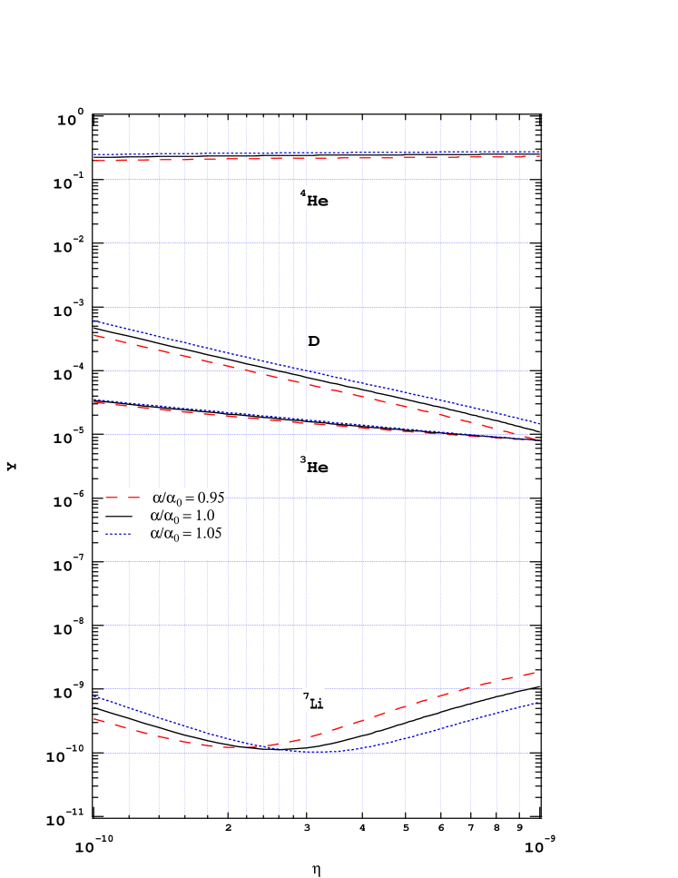
Figure 1: The abundances of the light elements $D$, ³He, ⁴He and ⁷Li as a function of $\eta$, the baryon-to-photon ratio. Curves are shown for the standard value of the fine structure constant $\alpha$, and for a variation of $\pm$ 5 % of the standard value. The results for the individual abundances are shown on an enlarged vertical scale in Figs. 2–3.

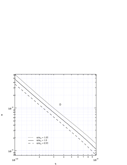
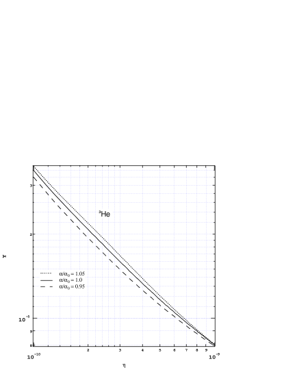
Figure 2: The abundance of (a) deuterium and (b) ³He as a function of $\eta$, the baryon-to-photon ratio. Curves are shown for the standard value of the fine structure constant $\alpha$, and for a variation of $\pm$ 5 % of the standard value.

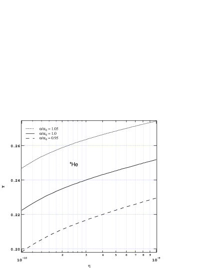
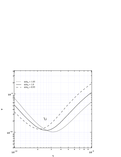
Figure 3: The abundance of (a) ⁴He and (b) ⁷Li as a function of $\eta$, the baryon-to-photon ratio. Curves are shown for the standard value of the fine structure constant $\alpha$, and for a variation of $\pm$ 5 % of the standard value.

In Fig. 1 we show the results for the final abundances of the observationally interesting elements ⁴He, ³He, $d$ and ⁷Li as a function of $\eta$, for SBBN and for a 5 % increase or decrease of the value of $\alpha$ during nucleosynthesis. In Figs. 2–3 the results for the abundances are shown separately on an expanded scale. As can be seen, the fractional change in the ⁴He abundance is quite insensitive to the value of $\eta$, as are the other abundances with the notable exception of ⁷Li. This is due to the two competing mechanisms for ⁷Li production, i.e., for $\eta\mathrel{\hbox to0.0pt{\lower 4.0pt\hbox{\hskip 1.0pt$\sim$}\hss}\raise 1.0pt\hbox{$<$}}3\times 10^{-10}$, ⁷Li is produced by ⁴He$(t,\gamma)^{7}$Li, a process in which the Coulomb-barrier is not as significant (but where the change in $\Delta m$ caused by a change in $\alpha$ is) as in the reaction ⁴He$(^{3}$He$,\gamma)^{7}$Be, which, followed by decay of ⁷Be to ⁷Li, is the dominant reaction that synthesizes ⁷Li for $\eta\mathrel{\hbox to0.0pt{\lower 4.0pt\hbox{\hskip 1.0pt$\sim$}\hss}\raise 1.0pt\hbox{$>$}}3\times 10^{-10}$.

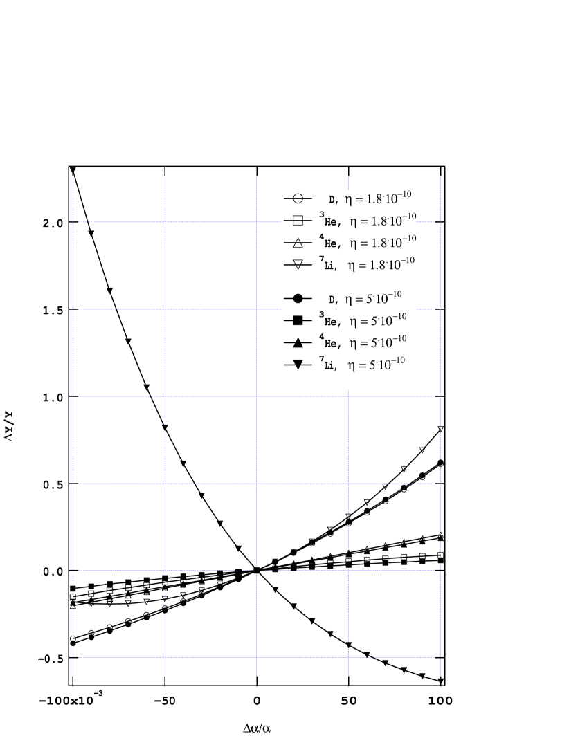
Figure 4: Fractional variation of the light-element abundances $Y$ vs fractional variation of the fine structure constant $\alpha$, for two values of the baryon-to-photon ratio $\eta$. Notice that the curves for ⁴He for the two $\eta$ values nearly overlap. The dramatic decrease of the ⁷Li abundance for a high $\eta$ value is due to the strong Coulomb barrier in its production.

Actually, the of $\eta$ coming from a comparison between the predictions of standard nucleosynthesis and observational data is presently quite uncertain, as is exemplified by the differing recent analyses of the problem in SBBN [21, 22]. In [21], a combined analysis gives $\eta\sim 1.8\cdot 10^{-10}$ (driven largely by accepting a high value of the deuterium abundance), whereas in [22] a low deuterium abundance is taken as the preferred observational result leading to a value $\eta\sim 5\cdot 10^{-10}$. In Fig. 4 the fractional changes in the light-element abundances are shown versus the assumed fractional change in $\alpha$ for both these values of $\eta$.

In the case of the low value of $\eta\sim 1.8\cdot 10^{-10}$, the ⁷Li abundance does not vary as strongly with a changing $\alpha$, and since this abundance is known less accurately than that of ⁴He it is the latter which has to be used to bound possible variations of $\alpha$. However, the observational status ⁴He is still a matter of debate, and it does not seem likely that the systematic errors are larger than usually quoted. For instance, the global fit referred to in [21] is

$$Y_{4}=0.238\pm 0.002\pm 0.005$$ (28)

whereas the corresponding value in a recent reanalysis by Izotov et al. [23] is given as

$$Y_{4}=0.244\pm 0.002$$ (29)

Using the second upper limit and the first lower limit for the ⁴He abundance, as is difficult to avoid before better data become available, we see from Fig. 3 (a) that a reduction of the value of $\alpha$ larger than 5 % is not excluded, if ⁴He is considered alone, and the other abundances are only used to generously bound $\eta$ to be in the interval $10^{-10}-10^{-9}$. Interestingly, one may note that on the contrary an increase of the electromagnetic strength by $2$ % would relieve the pressure these low-$\eta$ models feel from the upward revision of the ⁴He abundance of [23], while still falling in the allowed range for ⁷Li discussed below. Of course, we have to remember the fact that the change in ⁴He is caused by the model-dependent variation of the neutron-proton mass difference with $\alpha$.

For the high value of $\eta\sim 5\cdot 10^{-10}$, we see that a decrease of $\alpha$ by 2 % is within our allowed range of the ⁴He abundance (the change in deuterium caused by such a change in $\alpha$ does not affect very much the $\eta$ value assigned to a given deuterium measurement). Since for the high $\eta$ solution the variation of ⁷Li with $\alpha$ is rapid, we have to consider the observational data for lithium. Unfortunately, the situation is less than clear here as well. It seems that the data are well described by a “plateau” value versus metallicity, given by [24]

$$Y_{7}=\left(1.73\pm 0.30\right)\cdot 10^{-10}$$ (30)

The fact that there is little dispersion around this value could indicate that it represents the primordial abundance. However, lithium could be destroyed by stellar processes by an unknown amount, which has led some workers in the field [22] to consider the possibility that the true primordial value is up to a factor of 2 larger.

It is interesting to note from Fig. 1 that the ⁷Li abundance for this value of $\eta$ can be brought down to $2\cdot 10^{-10}$ if the strength of $\alpha$ was larger by around 3 % than the standard value (thus making the Coulomb suppression stronger). For the same change of $\alpha$, the ⁴He abundance is, however, violating our (model-dependent) upper bound by a considerable amount. Thus, we conclude that the high-$\eta$ solution, which already has problems explaining ⁷Li (if (30) represents the primordial value) can not be improved by changing $\alpha$, in contrast to the low-$\eta$ solution which may benefit from an increase of $\alpha$ by a couple of percent during nucleosynthesis.

6 Conclusions

The successful first-order comparison between Big Bang nucleosynthesis predictions and observed abundances implies that the values of the fundamental coupling constants at that epoch can not have been too much different from the present ones. When it comes to more precise statements, the situation is complicated by the presently partially conflicting measurements. (Similar conclusions have recently been obtained concerning possible limits on the effective number of neutrino species during nucleosynthesis [25].) We argue that it is impossible to quote a better bound than $2$ % on the deviation from the present value of $\alpha$ at the time of nucleosynthesis, and note that such a variation may even be implied, if the deuterium observations leading to the low-$\eta$ solution are confirmed with increased significance, and the trend continues of an increasing value for ⁴He from observations.

A new ingredient in our treatment is the discovery of the large sensitivity, especially at high values of $\eta$, of the ⁷Li abundance on the electromagnetic strength, due to exponential Coulomb barriers. If the experimental and theoretical situation is improved for this isotope, it holds the promise of giving the most stringent bound on variation of $\alpha$, with the added virtue that it is less sensitive to model assumptions than, e.g., ⁴He. The problem that the high-$\eta$ (low deuterium) solution may have in explaining the low plateau value of ⁷Li can in principle be solved by an increase in $\alpha$ by a few percent, but only if the true primordial ⁴He abundance is well above $0.25$ (or if $\Delta m$ depends on $\alpha$ in a different way than we have assumed).

It is of interest to notice that other exotic effects such as the presence of strong primordial magnetic fields mainly affect the ⁴He abundance [26] and not Li or the other elements. Also in this respect the signal given by ⁷Li is clearer.

The limit obtained here is about the same as the one potentially given by the recombination time test [10], but probably more significant since it is at a higher redshift. However, at the time when the microwave background was emitted, the universe was totally dominated by gravity and electromagnetic interactions from which it can be argued that it offers a less model-dependent test.

7 Acknowledgements

We thank Roberto Liotta for interesting discussions on the nuclear physics aspects of this problem. L.B. thanks the Swedish Natural Science Research Council for support, and S.I. is grateful to the Swedish Institute for a scholarship.

Number	Reaction	Reaction rate
$1$	${}^{2}H(p,\gamma)^{3}He$	$2.650\times 10^{3}(1+\delta)^{\frac{1}{3}}T_{9}^{-\frac{2}{3}}exp(-3.720(1+\delta)^{\frac{2}{3}}T_{9}^{-\frac{1}{3}})\times$
		$\times(1.000+1.120\times 10^{-1}(1+\delta)^{-\frac{2}{3}}T_{9}^{\frac{1}{3}}+1.990(1+\delta)^{\frac{2}{3}}T_{9}^{\frac{2}{3}}+1.560T_{9}+$
		$+1.620\times 10^{-1}(1+\delta)^{\frac{4}{3}}T_{9}^{\frac{4}{3}}+3.240\times 10^{-1}(1+\delta)^{\frac{2}{3}}T_{9}^{\frac{5}{3}})$
$2$	${}^{3}H(p,\gamma)^{4}He$	$2.200\times 10^{4}(1+\delta)^{\frac{1}{3}}T_{9}^{-\frac{2}{3}}exp(-3.869(1+\delta)^{\frac{2}{3}}T_{9}^{-\frac{1}{3}})\times$
		$\times(1.000+1.080\times 10^{-1}(1+\delta)^{-\frac{2}{3}}T_{9}^{\frac{1}{3}}+1.680(1+\delta)^{\frac{2}{3}}T_{9}^{\frac{2}{3}}+1.260T_{9}+$
		$+5.510\times 10^{-1}(1+\delta)^{\frac{4}{3}}T_{9}^{\frac{4}{3}}+1.060(1+\delta)^{\frac{2}{3}}T_{9}^{\frac{5}{3}})$
$3$	${}^{6}Li(p,\gamma)^{7}Be$	$6.690\times 10^{5}(1+\delta)^{\frac{1}{3}}T_{9a}^{\frac{5}{6}}T_{9}^{-\frac{3}{2}}exp(-8.413(1+\delta)^{\frac{2}{3}}T_{9a}^{-\frac{1}{3}})$
		$\left[T_{9a}=T_{9}/(1.000-9.690\times 10^{-2}T_{9}+2.000(1+\delta)^{\frac{2}{3}}T_{9}^{\frac{5}{3}}(1.000-9.690\times 10^{-2}T_{9})^{-\frac{2}{3}})\right]$
$4$	${}^{6}Li(p,\alpha)^{3}He$	$3.730\times 10^{10}(1+\delta)^{\frac{1}{3}}T_{9}^{-\frac{2}{3}}exp(-8.413(1+\delta)^{\frac{2}{3}}T_{9}^{-\frac{1}{3}}-(1.818\times 10^{-1}T_{9})^{2}(1+\delta)^{2})\times$
		$\times(1.000+5.000\times 10^{-2}(1+\delta)^{-\frac{2}{3}}T_{9}^{\frac{1}{3}}-6.100\times 10^{-2}(1+\delta)^{\frac{2}{3}}T_{9}^{\frac{2}{3}}-$
		$-2.100\times 10^{-2}T_{9}+6.000\times 10^{-3}(1+\delta)^{\frac{4}{3}}T_{9}^{\frac{4}{3}}+5.000\times 10^{-3}(1+\delta)^{\frac{2}{3}}T_{9}^{\frac{5}{3}})+$
		$+1.330\times 10^{10}T_{9}^{-\frac{3}{2}}exp(-1.776\times 10^{1}T_{9}^{-1})+$
		$+1.290\times 10^{9}T_{9}^{-1}exp(-2.182\times 10^{1}T_{9}^{-1})$
$5$	${}^{7}Li(p,\alpha)^{4}He$	$1.096\times 10^{9}(1+\delta)^{\frac{1}{3}}T_{9}^{-\frac{2}{3}}exp(-8.472(1+\delta)^{\frac{2}{3}}T_{9}^{-\frac{1}{3}})-$
		$-4.830\times 10^{8}(1+\delta)^{\frac{1}{3}}T_{9b}^{\frac{5}{6}}T_{9}^{-\frac{3}{2}}exp(-8.472(1+\delta)^{\frac{2}{3}}T_{9b}^{-\frac{1}{3}})+$
		$+1.060\times 10^{10}T_{9}^{-\frac{3}{2}}exp(-3.044\times 10^{1}T_{9}^{-1})+$
		$+1.560\times 10^{5}(1+\delta)^{\frac{1}{3}}T_{9}^{-\frac{2}{3}}exp((-8.472(1+\delta)^{\frac{2}{3}}T_{9}^{-\frac{1}{3}})-(5.896\times 10^{-1}T_{9})^{2}(1+\delta)^{2})\times$
		$\times(1.000+4.900\times 10^{-2}(1+\delta)^{-\frac{2}{3}}T_{9}^{\frac{1}{3}}-2.498(1+\delta)^{\frac{2}{3}}T_{9}^{\frac{2}{3}}+$
		$+8.600\times 10^{-1}T_{9}+3.518(1+\delta)^{\frac{4}{3}}T_{9}^{\frac{4}{3}}+3.080(1+\delta)^{\frac{2}{3}}T_{9}^{\frac{5}{3}})+$
		$+1.550\times 10^{6}T_{9}^{-\frac{3}{2}}exp(-4.478T_{9}^{-1})$
		$\left[T_{9b}=T_{9}/(1.000+0.759T_{9})\right]$
$6$	${}^{2}H(\alpha,\gamma)^{6}Li$	$3.010\times 10^{1}(1+\delta)^{\frac{1}{3}}T_{9}^{-\frac{2}{3}}exp(-7.423(1+\delta)^{\frac{2}{3}}T_{9}^{-\frac{1}{3}})\times$
		$\times(1.000+5.600\times 10^{-2}(1+\delta)^{-\frac{2}{3}}T_{9}^{\frac{1}{3}}-4.850(1+\delta)^{\frac{2}{3}}T_{9}^{\frac{2}{3}}+8.850T_{9}-$
		$-5.850\times 10^{-1}(1+\delta)^{\frac{4}{3}}T_{9}^{\frac{4}{3}}-5.840\times 10^{-1}(1+\delta)^{\frac{2}{3}}T_{9}^{\frac{5}{3}})+$
		$+8.550\times 10^{1}T_{9}^{-\frac{3}{2}}exp(-8.228T_{9}^{-1})$

Table 1: Reaction rates (in units of cm³s^-1mole^-1) for the most relevant $\alpha$-dependent reactions involved in SBBN (reactions 1-6). $T_{9}$ is the temperature in units of $10^{9}$ Kelvin.

Number	Reaction	Reaction rate
$7$	${}^{3}H(\alpha,\gamma)^{7}Li$	$3.032\times 10^{5}(1+\delta)^{\frac{1}{3}}T_{9}^{-\frac{2}{3}}exp(-8.090(1+\delta)^{\frac{2}{3}}T_{9}^{-\frac{1}{3}})\times$
		$\times(1.000+5.160\times 10^{-2}(1+\delta)^{-\frac{2}{3}}T_{9}^{\frac{1}{3}}+2.290\times 10^{-2}(1+\delta)^{\frac{2}{3}}T_{9}^{\frac{2}{3}}+$
		$+8.280\times 10^{-3}T_{9}-3.280\times 10^{-4}(1+\delta)^{\frac{4}{3}}T_{9}^{\frac{4}{3}}-3.010\times 10^{-4}(1+\delta)^{\frac{2}{3}}T_{9}^{\frac{5}{3}})+$
		$+5.109\times 10^{5}(1+\delta)^{\frac{1}{3}}T_{9c}^{\frac{5}{6}}T_{9}^{-\frac{3}{2}}exp(-8.068(1+\delta)^{\frac{2}{3}}T_{9c}^{-\frac{1}{3}})$
		$\left[T_{9c}=T_{9}/(1.000+0.138T_{9})\right]$
$8$	${}^{3}He(\alpha,\gamma)^{7}Be$	$4.817\times 10^{6}(1+\delta)^{\frac{1}{3}}T_{9}^{-\frac{2}{3}}exp(-1.496\times 10^{1}(1+\delta)^{\frac{2}{3}}T_{9}^{-\frac{1}{3}})\times$
		$\times(1.000+3.250\times 10^{-2}(1+\delta)^{-\frac{2}{3}}T_{9}^{\frac{1}{3}}-1.040\times 10^{-3}(1+\delta)^{\frac{2}{3}}T_{9}^{\frac{2}{3}}-$
		$-2.370\times 10^{-4}T_{9}-8.110\times 10^{-5}(1+\delta)^{\frac{4}{3}}T_{9}^{\frac{4}{3}}-4.690\times 10^{-5}(1+\delta)^{\frac{2}{3}}T_{9}^{\frac{5}{3}})+$
		$+5.938\times 10^{6}(1+\delta)^{\frac{1}{3}}T_{9d}^{\frac{5}{6}}T_{9}^{-\frac{3}{2}}exp(-1.286\times 10^{1}(1+\delta)^{\frac{2}{3}}T_{9d}^{-\frac{1}{3}})$
		$\left[T_{9d}=T_{9}/(1.000+0.107T_{9})\right]$
$9$	${}^{2}H(d,n)^{3}He$	$3.950\times 10^{8}(1+\delta)^{\frac{1}{3}}T_{9}^{-\frac{2}{3}}exp(-4.259(1+\delta)^{\frac{2}{3}}T_{9}^{-\frac{1}{3}})\times$
		$\times(1.000+9.800\times 10^{-2}(1+\delta)^{-\frac{2}{3}}T_{9}^{\frac{1}{3}}+7.650\times 10^{-1}(1+\delta)^{\frac{2}{3}}T_{9}^{\frac{2}{3}}+$
		$+5.250\times 10^{-1}T_{9}+9.610\times 10^{-3}(1+\delta)^{\frac{4}{3}}T_{9}^{\frac{4}{3}}+1.670\times 10^{-2}(1+\delta)^{\frac{2}{3}}T_{9}^{\frac{5}{3}})$
$10$	${}^{2}H(d,p)^{3}H$	$4.170\times 10^{8}(1+\delta)^{\frac{1}{3}}T_{9}^{-\frac{2}{3}}exp(-4.258(1+\delta)^{\frac{2}{3}}T_{9}^{-\frac{1}{3}})\times$
		$\times(1.000+9.800\times 10^{-2}(1+\delta)^{-\frac{2}{3}}T_{9}^{\frac{1}{3}}+5.180\times 10^{-1}(1+\delta)^{\frac{2}{3}}T_{9}^{\frac{2}{3}}+$
		$+3.550\times 10^{-1}T_{9}-1.000\times 10^{-2}(1+\delta)^{\frac{4}{3}}T_{9}^{\frac{4}{3}}-1.800\times 10^{-2}(1+\delta)^{\frac{2}{3}}T_{9}^{\frac{5}{3}})$
$11$	${}^{3}H(d,n)^{4}He$	$1.063\times 10^{11}(1+\delta)^{\frac{1}{3}}T_{9}^{-\frac{2}{3}}exp(-4.559(1+\delta)^{\frac{2}{3}}T_{9}^{-\frac{1}{3}}-(1.326\times 10^{1}T_{9})^{2}(1+\delta)^{2})\times$
		$\times(1.000+9.200\times 10^{-2}(1+\delta)^{-\frac{2}{3}}T_{9}^{\frac{1}{3}}-3.750\times 10^{-1}(1+\delta)^{\frac{2}{3}}T_{9}^{\frac{2}{3}}-$
		$-2.420\times 10^{-1}T_{9}+3.382\times 10^{1}(1+\delta)^{\frac{4}{3}}T_{9}^{\frac{4}{3}}+5.542\times 10^{1}(1+\delta)^{\frac{2}{3}}T_{9}^{\frac{5}{3}})+$
		$+8.047\times 10^{8}T_{9}^{-\frac{2}{3}}exp(-0.486T_{9}^{-1})$
$12$	${}^{3}He(d,p)^{4}He$	$5.021\times 10^{10}(1+\delta)^{\frac{1}{3}}T_{9}^{-\frac{2}{3}}exp(-7.144(1+\delta)^{\frac{2}{3}}T_{9}^{-\frac{1}{3}}-(3.704T_{9})^{2}(1+\delta)^{2})\times$
		$\times(1.000+5.800\times 10^{-2}(1+\delta)^{-\frac{2}{3}}T_{9}^{\frac{1}{3}}+6.030\times 10^{-1}(1+\delta)^{\frac{2}{3}}T_{9}^{\frac{2}{3}}+$
		$+2.450\times 10^{-1}T_{9}+6.970(1+\delta)^{\frac{4}{3}}T_{9}^{\frac{4}{3}}+7.190(1+\delta)^{\frac{2}{3}}T_{9}^{\frac{5}{3}})+$
		$+5.212\times 10^{8}T_{9}^{-\frac{1}{2}}exp(-1.762T_{9}^{-1})$

Table 2: Reaction rates (in units of cm³s^-1mole^-1) for the most relevant $\alpha$-dependent reactions involved in SBBN(reactions 7-12). $T_{9}$ is the temperature in units of $10^{9}$ Kelvin.

References

- [1] P. A. M. Dirac, Nature 139, 323 (1937).
- [2] Particle Data Group, C. Caso et al., Eur. Phys. J. C 3, 1 (1998).
- [3] E. W. Kolb, J. M. Perry and T. P. Walker, Phys. Rev. D 33, 869 (1986).
- [4] J. D. Prestage, R. L. Tjoelker and L. Maleki, Phys. Rev. Lett. 74, 3511 (1985).
- [5] J. K. Webb, V. V. Flambaum, C. W. Churchill, M. J. Drinkwater and J. D. Barrow, astroph/9803165 (1998); M. J. Drinkwater, J. K. Webb, J. D. Barrow and V. V. Flambaum, Mon. Not. Roy. Astron. Soc. 295, 457 (1998); L. L. Cowie and A. Songaila, Astrophys. J. 453, 596 (1995).
- [6] T. Damour and F. Dyson, Nucl. Phys. B 480, 37 (1996).
- [7] W. J. Marciano, Phys. Rev. Lett. 52 489 (1984).
- [8] G. Veneziano, Proc. of the Nobel Symposium “Particle Physics and the Universe”, to appear in Physica Scripta (L. Bergström, P. Carlson and C. Fransson, eds.).
- [9] T. Damour and A. M. Polyakov, Nuc Phys. B 423, 532 (1994).
- [10] M. Kaplinghat, R. J. Scherrer, M. S. Turner, astro-ph/9810133 (1998); S. Hannestad, astro-ph/9810102 (1998).
- [11] E. W. Kolb and M. S. Turner, “The Early Universe”, Addison-Wesley Publishing Company (1990).
- [12] M. S. Smith, L. H. Kawano and R. A. Malaney, Astrophys. J. Suppl. 85, 219 (1993).
- [13] D. A. Dicus, E. W. Kolb, A. M. Glesson, E. C. G. Sudarshan, V. L. Teplitz and M. S. Turner, Phys. Rev. D 26, 2694 (1982).
- [14] L. H. Kawano, FERMILAB-PUB-88/34-A, preprint (1988); FERMILAB-PUB-92/04-A, preprint (1992).
- [15] V. V. Dixit and M. Sher, Phys. Rev. D 37, 1097 (1988).
- [16] B. A. Campbell and K. A. Olive, Phys. Lett. B 345, 429 (1995).
- [17] J. Gasser and H. Leutwyler, Phys. Rep. 87, 77 (1982).
- [18] W. A. Fowler, G. R. Caughlan and B. A. Zimmerman, Ann. Rev. Astron. Astroph. 5, 525 (1967); W. A. Fowler, G. R. Caughlan and B. A. Zimmerman, Ann. Rev. Astron. Astroph. 13, 69 (1975).
- [19] H. Oberhummer, H. Herndl, T. Rauscher and H. Beer, Surveys in Geophysics, 17, 665 (1996).
- [20] H. J. Haubold and A. M. Mathai, Studies App. Math. 75, 123 (1986); H. J. Haubold and A. M. Mathai, astro-ph/9612011 (1996).
- [21] K. A. Olive, astro-ph/9901231 (1999).
- [22] S. Burles, K. M. Nollett, J. N. Truran and M. S. Turner, astro-ph/9901157 (1999).
- [23] Y. Izotov, T. Thuan and V. Lipovetsky, Astrophys. J. Suppl. 108, 1 (1997).
- [24] P. Bonifacio and P. Molaro, Mon. Not. Roy. Astron. Soc. 285, 847 (1997).
- [25] E. Lisi, S. Sarkar and F.L. Villante, hep-ph/9901404.
- [26] D. Grasso and H. R. Rubinstein, Phys. Lett. B 379, 73 (1996).