Building galaxy models with Schwarzschild method and spectral dynamics

Abstract

Tremendous progress has been made recently in modelling the morphology and kinematics of centers of galaxies. Increasingly realistic models are built for central bar, bulge, nucleus and black hole of galaxies, including our own. The newly revived Schwarzschild method has played a central role in these theoretical modellings. Here I will highlight some recent work at Leiden on extending the Schwarzschild method in a few directions. After a brief discussion of (i) an analytical approach to include stochastic orbits (Zhao 1996), and (ii) the “pendulum effect” of loop and boxlet orbits (Zhao, Carollo, de Zeeuw 1999), I will concentrate on the very promising (iii) spectral dynamics method, with which not only can one obtain semi-analytically the actions of individual orbits as previously known, but also many other physical quantities, such as the density in configuration space and the line-of-sight velocity distribution of a superposition of orbits (Copin, Zhao & de Zeeuw 1999). The latter method also represents a drastic reduction of storage space for the orbit library and an increase in accuracy over the grid-based Schwarzschild method.

1 Introduction

One of the classical problems in galaxy dynamics is building equilibrium models for a galaxy with an observed light distribution. The basic process can be illustrated by the simpliest form of the problem, which is to construct a spherical, isotropic model with a constant mass-to-light ratio $M/L$ and a stellar distribution function $DF$ which fits the light profile. This has the well-known solution (Eddington 1916),

$$DF(E)\propto\int_{E}^{0}{d^{2}\rho\over d\phi^{2}}{d\phi\over\sqrt{\phi-E}},$$ (1)

which is a function of the energy $E$ only, where the potential $\phi$ comes from solving the Poisson equation, and the volume density $\rho(r)$ comes from deprojecting the light profile $\mu(R)$

$$\rho(r)\propto{M\over L}\int_{r}^{\infty}{d\mu(R)\over dR}{dR\over\sqrt{R^{2}-r^{2}}}.$$ (2)

In general deprojecting the light and getting the potential are relatively easier parts of the problem.

While a simple problem in concept, it is challenging to extend the mathematical and numerical machinery to cope with realistic systems. In particular, galaxies are almost always flattened, and sometimes triaxial. They are also anisotropic in velocity distribution due to dissipational and dissipationless processes in formation. By formation they are often dominated by dark matter at very small and very large radii (central black holes as indicated by nuclear activities in AGNs and outer dark halos as by flat HI rotation curves). In short, none of the three simplifying assumptions (constant $M/L$, isotropic and spherical) are generally valid.

While progress has been made in the analytical direction, the application is generally limited. The Hunter & Qian (1993) method, for example, can construct two-integral models – with a DF being function of energy and angular momentum azimuthal component $DF(E,L_{z})$ – for axisymmetric galaxies and has been applied, e.g., in the case of the nucleus of M32 (Qian et al. 1995. See also, Dejonghe 1986, Dehnen & Gerhard 1994 for alternative techniques of building two-integral models). Formulaism also exists for building anisotropic non-axisymmetric models as long as the potential remains in Stäckel form (Teuben 1987, Statler 1987, 1991, Arnold et al. 1994, Dejonghe et al. 1995), and in a few cases for tumbling models (e.g. Freeman 1966, Vandervoort 1980). As a side comment separability is no guarantee for self-consistency; for example, the recent non-axisymmetric disc potentials by Sridhar & Touma (1997) require unphysically negative DF (Syer & Zhao 1998).

At the other end of the spectrum of methods straight N-body simulations can deal with all geometries (Aarseth & Binney 1976, Wilkinson & James 1982, Barnes 1996), but their power is again limited when it comes to sculpturing a simulation to fit a set of observations in certain $\chi^{2}$ sense. The limitation here is the huge amount of computation to cover enough degrees of freedom to find the true best fitting model, e.g. Fux’s models (1997) for the Milky Way.

The most promising approach so far is the so-called Schwarzschild (1979) method, after his pioneering efforts in this direction. Basically one tries to match the observed distribution of the light with typically a few hundred or thousand building blocks with each being one stellar orbit populated with certain amount of stars. One adjusts the mass assigned to each orbit until a best match is obtained (see reviews by Binney 1982, de Zeeuw & Franx 1991, de Zeeuw 1996, Merritt 1996, 1999).

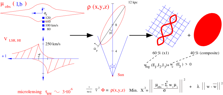
Figure 1: An illustration of the steps in building a bar model for the Milky Way with a modified Schwarzschild method. We start from (1) a dust-corrected near infrared surface brightness map $\mu_{obs}(l,b)$ of the Galaxy from COBE/DIRBE observations, (2) the velocity dispersion $\sigma_{r}$ measurements on the minor axis of the Galaxy, (3) the atomic hydrogen intensity map in the longitude $l$ vs. line of sight velocity plane, which is basically a measure of the rotation curve $V_{LSR,HI}$ of the Galaxy, and (4) the probability (optical depth) of microlensing $\tau_{BW}$ towards the Baade Window ($l=1^{o},b=-4^{o}$). We then use these input quantities to build the potential $\Phi(x,y,z)$ of the bar via the Poisson equation, and constrain the axis ratio and the orientation of the bar. Finally we seek a positive DF of regular orbits ($x_{1}$, $x_{2}$, $x_{4}$ orbits etc.) of weights $w(E_{J},I_{2},I_{3})$ plus super-orbits (composite orbits) of weights $w(E_{J})$ such that the ensemble $\sum_{i}^{N}w_{i}\mu_{i}$ matches the observed distribution $\mu_{obs}$ in a set of rectangular grid cells. The last step is a $\chi^{2}$ minimization problem, regularized by slightly ($\lambda\sim 10^{-4}$) penalizing DF where adjacent orbits in phase space have wildly different weights $w_{i}$. We feed the final model to an N-body code to test stability.

2 Schwarzschild method with bells & whistles

The Schwarzschild method has now been extensively applied to study nearby elliptical and S0 galaxies under the assumption of a static spherical, axisymmetric or triaxial potential (e.g., Richstone & Tremaine 1988, Merritt & Fridman 1996, Rix et al. 1997, van der Marel et al. 1998), and has also been applied to build 2-dimensional models of external bars (Pfenniger 1984, Wozniak & Pfenniger 1997, see also Sellwood & Wilkinson 1993) and 3-dimensional models of the tumbling bar of our own galaxy (Zhao 1996). These applications have also greatly generalized the original layout of the Schwarzschild method, and in particular, it is possible to match the orbits to a variety of kinematic data of gas and stars, and to derive a smooth physical solution (cf. the schematic Fig. 1). Nevertheless there are three main limitations of Schwarzschild approach and these are best overcome by joining force with the analytical and the N-body approaches.

Limitation A: Stability of a Schwarzschild model needs to be addressed by an N-body simulation. An interesting idea, due to Syer & Tremaine (1996) is to do the $\chi^{2}$ fitting and N-body simulation at the same time, adjusting the mass of each particle as the simulation evolves towards a best match of data with the distribution of the particles. A simpler, better understood approach is to design a Schwarzschild model first, then populate each library orbit with $N_{\bf A}$ particles with random phase where $N_{\bf A}$ is proportional to the weight assigned to the orbit with actions ${\bf A}$, and finally feed these particles to an N-body simulation code to test stability. This has been applied successfully to the Galactic bar, which is found to be stable (Zhao 1996).

Limitation B: Stochastic orbits in a Schwarzschild model make the model evolve on time scales of the mixing time (several hundred dynamical time, cf. Merritt & Valluri 1996). Merritt & Fridman (1996) propose to average out this effect by explicitly summing up many stochastic orbits to achieve a good phase-mix. This is challenging because it means integrating a few hundred orbits for a few thousand of dynamical times to beat down the time-dependent fluctuations. An alternative approach has been used in the case of the Galactic bar (Zhao 1996). The hybrid model makes use of two types of building blocks for the Galaxy (cf. Fig. 1): a library of regular orbits obtained by direct integration for several hundred dynamical time, and a library of “super-orbits”, which are nothing but many delta-like DFs $\sum_{i}N_{i}\delta(E_{J}-i\Delta)$, where the weighting $N_{i}$ are to be found by the same Non-Negative Least Square fitting code as with the weighting of the regular orbits. Each delta function includes all orbits with the same Jacobi integral $E_{J}\equiv E-\Omega J_{z}$ implicitly, where $\Omega$ is the tumbling speed of the bar and $E_{J}$ is the only analytical integral. Such a prescription naturally incorporates stochastic orbits in the model without explicitly making the division of the fraction of mass in stochastic orbits vs. regular ones. Variations of our analytical way of including stochastic orbits have now been developed to model axisymmetric systems and bars by the dynamics groups at Leiden (Cretton et al. 1998, private communication) and Oxford (Häfner et al. 1998, private communication).

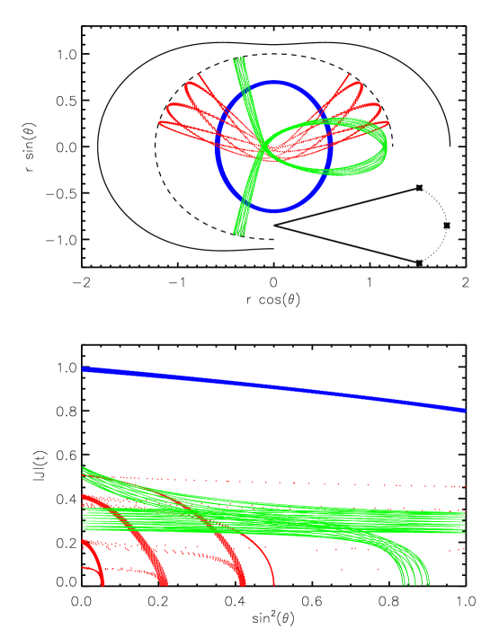
Figure 2: the upper panel shows three types of centro-phobic orbits: a loop orbit (thick band), a banana orbit (dotted lines) and a fish orbit (solid thin lines) together with the iso-density and iso-potential contours (heavy solid and dashed lines respectively). The lower panel shows the angular momentum $|J(t)|$ of a star as a function of the angle from the major axis ($\theta=0$) along the same three orbits, where each dot is one time step of the orbit. Note that $|J(t)|$ peaks on approaching the major axis for all boxlet orbits, like it does for the loops and the pendulum. A pendulum with a variable length is also sketched in the upper panel.

Limitation C: A Schwarzschild model is cell-dependent. Checking self-consistency of the model involves computing the amount of time an orbit spends inside a cell and comparing it with the amount of mass prescribed in the same cell. However it is possible to make cell-independent modeling. For example, to keep a triaxial galaxy in equilibrium requires a healthy mix of shapes of its building blocks with some orbits more flattened than the potential, some less flattened. It is well-known that loop orbits cannot reproduce a self-consistent triaxial potential because they move too fast and spend too little time at the major axis to match the relatively (compared to, say, the minor axis) high model density there. We find that this problem is actually more general (Zhao, Carollo & de Zeeuw 1999): it is easy to prove analytically that any regular orbit will reach a local maximum for its angular momentum $|J(t)|$ at the major axis, because the torque of triaxial potential is always directed towards the major axis (cf. Fig. 2). So in this regard a loop orbit or a boxlet orbit (with the shape of a banana, fish, pretzel etc) behaves like a pendulum with a stretchable length. Since a pendulum tends to swing too fast and spend too little time at its symmetry axis, the ”pendulum effect” generally prevents loops and boxlets from putting many stars at the major axis. This can be used as a cell-independent argument against making strongly flattened and triaxial galactic nuclei with bananas, fishes etc., consistent with previous authors (e.g., Gerhard & Binney 1985, Pfenniger & de Zeeuw 1989).

3 Spectral dynamics method

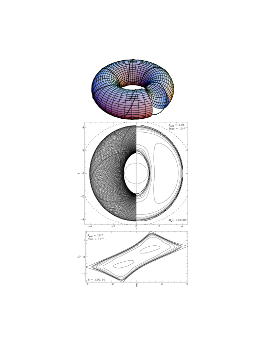
Figure 3: A planar loop orbit in various cuts of the phase space. The top panel shows the phase space torus of the orbit, which will be populated uniformly after integrating the orbit for a long time. The orbit in the configuration space is related to the torus by eq. (3), and the uniformly populated torus projects to a non-uniform distribution in the configuration space via a Jacobian (cf. eq. 6). The middle panel shows the reconstructed orbit in the $xy$ plane, folded to the left half, and the density contour map of the orbit, folded to the right half. The bottom panel shows the line of sight velocity distribution of the orbit in the impact parameter $x$ vs. velocity $v_{y}$ plane, computed with eq. (7); the tiled parallelogram is indicative of the rotation of the loop (Copin et al. 1999).

Another very promising cell-independent method of building galaxies is the spectral dynamics method. This method, as introduced by Binney & Spergel (1982), provides a conceptually simple representation of a regular orbit, by decomposing it into a truncated Fourier series involving three fundamental frequencies. The basic idea here is that a regular orbit in a 3D potential is simplest described in the action angle space since it satisfies periodic boundary conditions on the torus (cf. Fig. 3). Let an orbit be labeled by its three actions ${\bf A}$, then the phase space coordinates $[{\bf x}_{\bf A}(t),{\bf v}_{\bf A}(t)]$ are periodic with respect to the three action angles $\theta\equiv(\omega_{1},\omega_{2},\omega_{3})t$, ie., we have the following truncated Fourier series

$${\bf x}_{\bf A}(t)=\sum_{\lambda\equiv(l,m,n)}^{L}X_{\lambda}\cos(\lambda\cdot\theta+\chi_{\lambda}),~{}~{}\theta\equiv(\omega_{1},\omega_{2},\omega_{3})t.$$ (3)

where the $\omega$’s are the three basic frequencies, the coefficients $X_{\lambda}$ are the amplitudes of each frequency combination and $L$ is the highest order harmonics before truncation. Similarly the velocity of the orbit at any time, related to the position by a time derivative, can be written down as

$${\bf v}_{\bf A}(t)=-\sum_{\lambda\equiv(l,m,n)}^{L}\omega_{\lambda}X_{\lambda}\sin(\lambda\cdot\theta+\chi_{\lambda}),~{}~{}\omega_{\lambda}=l\omega_{1}+m\omega_{2}+n\omega_{3},$$ (4)

It is easy to work out the actions ${\bf A}$ by integrating along one of the three action angles,

$${\bf A}={1\over 2}\sum_{\lambda}X_{\lambda}^{2}(l\omega_{1},m\omega_{2},n\omega_{3}).$$ (5)

This method actually goes back to many years ago (e.g., Ratcliff, Chang & Schwarzschild 1984), but recent work by the Oxford group (e.g., Kaasalainen & Binney 1994), and by Papaphilipou & Laskar (1996) and Carpintero & Aguilar (1998) has made it possible to extract the basic frequencies numerically from the time series data of a regular orbit. Namely the step from $[{\bf x}_{\bf A}(i\Delta t),{\bf v}_{\bf A}(i\Delta t)]$ to $[\omega_{\lambda},X_{\lambda}]$.

Most important to the Schwarzschild method is that we can compute the volume density of the orbit ${\bf A}$ at a given point $(x,y,z)$. Since we know that a regular orbit is uniformly distributed in its action angle space, the density in the real space is given by

$$\rho_{\bf A}(x,y,z)={1\over(2\pi)^{3}}\left|{\partial(x,y,z)\over\partial(\theta_{1},\theta_{2},\theta_{3})}\right|^{-1},$$ (6)

where the partial derivatives are simply the Jacobian for the transformation between the action angle space $(\theta_{1},\theta_{2},\theta_{3})$ and the coordinate space $(x,y,z)$. Since the Jacobian can be evaluated analytically with eq. (3), we have derived a rigorous expression for the spatial distribution of an orbit. Likewise the line-of-sight velocity ($v_{z}$) distribution of an orbit in the direction $(x,y)$ (cf. Fig. 3) is given by

$$LOSVD_{\bf A}(x,y,v_{z})={1\over(2\pi)^{3}}\left|{\partial(x,y,v_{z})\over\partial(\theta_{1},\theta_{2},\theta_{3})}\right|^{-1}.$$ (7)

For details see Copin et al. (1999).

The beauty of this method is that the description of regular orbits is conceptually simple. The description is time-independent, and involves no gridding and binning. It is also easy to store and recover an orbit, thus saving the amount of disc space for storing orbit libraries. Typically the number of quantities to store is about $10$ times the dimension of the problem; this includes the basic frequencies and the leading amplitudes.

To conclude we remark that the most promising method might be some kind of generalized Schwarzschild method or hybrid method, where the computationally intentive stochastic orbits are implicitly modelled by the analytical super-orbits, and the spatial and velocity distribution of the regular orbits are treated with spectral dynamics.

I thank Tim de Zeeuw for a critical reading of an earlier version and Danny Pronk for making the electronic version of Figure 1.

References

- [1] Aarseth S. & Binney J. 1976, MNRAS, 185, 227
- [2] Arnold R., de Zeeuw P.T., & Hunter C. 1994, MNRAS 271, 924
- [3] Barnes J. 1996, in the formation of Galaxies, Proc. 5th Carnary Islands Winter School of Astrophysics, ed. C. Munoz-Tunon (Cambridge: Cambridge U. Press), p399
- [4] Binney J., 1982, ARAA, 20, 399
- [5] Binney J., Spergel, D., 1982, ApJ, 252, 308
- [6] Carpintero D.D., Aguilar L.A., 1998, MNRAS, 298, 1
- [7] Copin Y., Zhao H. & de Zeeuw P.T. 1999, in preparation
- [8] de Zeeuw P.T. 1996, in Gravitational Dynamics, Proc. 36th Herstmonceux Conf., ed. O. Lahav, E. Terlevich & R.J. Terlevich, Cambridge U. Press, p1
- [9] de Zeeuw P.T. & Franx M. 1991, ARAS, 29, 239
- [10] Merritt D. 1996, in The Nature of Elliptical Galaxies, 2nd Stromlo Symposium, ed. M. Arnaboldi, G. Da Costa and P. Saha (astro-ph/9611082)
- [11] Merritt D. 1999, PASP, 111, 129 (astro-ph/9810371)
- [12] Dehnen W. & Gerhard O. 1994, MNRAS, 268, 1019
- [13] Dejonghe H. 1986, Phys. Rep. 133, 217
- [14] Dejonghe H. et al. 1995, A&A, 306, 363
- [15] Eddington A. S. 1916, MNRAS 76, 572
- [16] Freeman K. 1966, MNRAS, 134, 15
- [17] Fux R. 1997, A&A 327, 983
- [18] Gerhard O. 1994, in Galactic Dynamics & N-body Simulations, Proc. 6th European Summer School, ed. G. Contopoulos & G. Spyrou (New York: Springer), p191
- [19] Gerhard O.E. & Binney J.J., 1985, MNRAS, 216, 467
- [20] Hunter C. & Qian E. 1993, MNRAS, 262, 401
- [21] Kaasalainen M. & Binney J. 1994, MNRAS, 268, 1033
- [22] Merritt D.R., Fridman T., 1996, ApJ, 460, 136
- [23] Merritt D.R., Valluri M., 1996, ApJ, 471, 82
- [24] Papaphilipou, Y., Laskar, J., 1996, A&A, 307, 427
- [25] Pfenniger D. 1984, A&A, 141, 171
- [26] Pfenniger D., de Zeeuw P.T., 1989, in Dynamics of Dense Stellar Systems, ed. Dave Merritt, Cambridge Univ. Press, p81
- [27] Qian E.E. et al. 1995, MNRAS, 274, 602
- [28] Ratcliff S.J., Chang K.M. & Schwarzschild M. 1984, ApJ, 279, 610
- [29] Richstone, D. & Tremaine, S. 1988, ApJ, 327, 82
- [30] Rix H.-W. et al. 1997, ApJ, 488, 706
- [31] Schwarzschild M., 1979, ApJ, 232, 236
- [32] Sellwood J. & Wilkinson A. 1993, Rep. Prog. Phys. 56, 173
- [33] Sridhar S., Touma J., 1997, MNRAS, 287, L1
- [34] Statler T. S., 1987, ApJ, 321, 113
- [35] Statler T. S., 1991, A.J., 102, 882
- [36] Syer D., Zhao H.S., 1998, MNRAS, 296, 407
- [37] Teuben P. 1987 MNRAS, 227, 815
- [38] van der Marel R.P. et al. 1998, ApJ 493, 613
- [39] Vandervoort P.O., 1980, ApJ, 240, 478
- [40] Wilkinson A. & James R.A. 1982, MNRAS, 199, 171
- [41] Wozniak H. & Pfenniger D. 1997, A&A, 317, 14
- [42] Zhao H.S., 1996, MNRAS, 283, 149
- [43] Zhao H.S., Carollo C.M. & de Zeeuw P.T. 1999, MNRAS, 304, 457