Projection effects in mass-selected galaxy-cluster samples

Abstract

Selection of galaxy clusters by mass is now possible due to weak gravitational lensing effects. It is an important question then whether this type of selection reduces the projection effects prevalent in optically selected cluster samples. We address this question using simulated data, from which we construct synthetic cluster catalogues both with Abell’s criterion and an aperture-mass estimator sensitive to gravitational tidal effects. The signal-to-noise ratio of the latter allows to some degree to control the properties of the cluster sample. For the first time, we apply the cluster-detection algorithm proposed by Schneider to large-scale structure simulations.

We find that selection of clusters through weak gravitational lensing is more reliable in terms of completeness and spurious detections. Choosing the signal-to-noise threshold appropriately, the completeness can be increased up to 100%, and the fraction of spurious detections can significantly be reduced compared to Abell-selected cluster samples.

We also investigate the accuracy of mass estimates in cluster samples selected by both luminosity and weak-lensing effects. We find that mass estimates from gravitational lensing, for which we employ the $\zeta$-statistics by Kaiser et al., are significantly more accurate than those obtained from galaxy kinematics via the virial theorem.

1 Introduction

Observed samples of galaxy clusters are notoriously contaminated by projection effects (Frenk et al. 1990) even when selected with respect to their X-ray emission (Bartelmann & Steinmetz 1996; van Haarlem, Frenk & White 1997; Cen 1997). This is particularly annoying because clusters constitute an important class of cosmological objects, and cleanly defined cluster samples could provide a wealth of cosmological information. Not only the definition of clusters within samples, but also observable cluster properties like their richness, X-ray luminosity, gas fraction, degree of substructure, velocity dispersion and the mass estimates derived therefrom can substantially be biased by projection effects.

While not solving the principal problem of observing aspherical three-dimensional objects in projection, selection of clusters by mass rather than luminosity might prove a substantial step towards more reliably defined cluster samples. With the advent of weak-lensing techniques and wide-field surveys, mass-selected cluster samples are beginning to come within reach. The tidal field of the total gravitating cluster mass determines the amount of distortion observed in images of background galaxies (Kaiser & Squires 1993). A variety of elaborate tools has been developed in the past few years to detect clusters and derive their masses utilising distortions of faint-galaxy samples (Fahlman et al. 1994; Kaiser 1995; Kaiser, Squires & Broadhurst 1995; Seitz & Schneider 1995; Bartelmann et al. 1996; Seitz & Schneider 1996; Squires & Kaiser 1996 to name just a few). In particular, weighted second-order measures of the distortion field in apertures like the aperture mass statistics ($M_{\rm ap}$-statistics) provide means to derive the signal-to-noise ratio $S$ of a measurement from the data themselves (Schneider 1996). A possible strategy to use aperture measures like $M_{\rm ap}$ for cluster detection is to move the aperture across a wide data field and monitor $M_{\rm ap}$ and $S$ as a function of aperture position. Points or regions of high $S$ can then be identified as potential clusters, leading to the definition of mass-selected cluster samples. This technique led to a cluster detection in the ESO Imaging Survey (T. Erben, private communication). A further spectacular example of galaxy clusters detected through weak lensing is given by Kaiser et al. (1998).

Strictly speaking, distortions caused by gravitational lensing trace the gravitational tidal field rather than the mass itself. This is due to the fact that a sheet of constant surface mass density added to any given lens does not change the shapes of distorted images, but only their sizes (the so-called mass-sheet degeneracy). Therefore, cluster detection techniques based on distortion measurements alone select clusters not by mass, but by the amplitude of their tidal field. Keeping this in mind, we will hereafter speak of mass-selected clusters in that sense.

The question then arises, are the cluster samples so obtained any more reliable than, e.g., cluster samples selected via Abell’s criterion or X-ray luminosity? More precisely, what fraction of true three-dimensional clusters is detected that way, and what fraction of the mass-selected samples are spurious detections, either not corresponding to real clusters at all or to clusters outside the desired mass range? This is the question addressed in this paper using simulated $N$-body data, to which we apply for the first time the $M_{\rm ap}$ statistics to construct synthetic cluster samples.

We use high-resolution large-scale structure simulations and first identify three-dimensional clusters in real space. We then populate the simulation volume with galaxies, fixing the average mass-to-light ratio. In projection, we apply Abell’s criterion to construct optically-selected cluster samples for comparison, and the $S$-statistics to define mass-selected cluster samples via the gravitational lensing effects of the simulated matter distribution. The quality of the mass-selected samples is then assessed in comparison to that of the optically-selected samples. Moreover, we derive masses both from galaxy kinematics and weak lensing to compare the reliability of the different mass estimates.

Section 2 details the methods used. Section 3 discusses the quality of the cluster samples in terms of completeness and the fraction of spurious detections. In Sect. 4 and in the Appendix, we give examples for the line-of-sight structure of some representative mass-selected clusters. Mass estimates are presented and discussed in Sect. 5, and Sect. 6 summarises our conclusions.

2 Methods

2.1 $N$-body simulation

In order to study the influence of projection effects on cluster surveys selected by optical and gravitational lensing information, we need simulated data allowing to mimic as accurately as possible the selection of clusters and the determination of their properties, for instance their masses. At the same time, the full phase-space information is required to assess the amount of contamination of selected clusters by intervening matter along the line-of-sight (hereafter los). For this purpose, we use a large, high-resolution $N$-body simulation of a standard Cold Dark Matter (SCDM) universe. The simulation was carried out within the GIF project (Kauffmann et al. 1998) using a parallelised version of the HYDRA code. HYDRA (Couchman, Pearce & Thomas 1995; Couchman, Thomas & Pearce 1996) is an adaptive particle-particle particle-mesh (AP³M) code. It uses direct force summation in clustered regions, whereas long-range forces and forces within weakly clustered regions are computed on a mesh. The simulation used here transports $256^{3}$ particles in a periodic comoving cubic volume of $(85\,h^{-1}\,{\rm Mpc})^{3}$, where $h$ is the Hubble constant in units of $100\,{\rm km\,s^{-1}\,Mpc^{-1}}$.

The simulation adopts the approximation to the linear CDM power spectrum (Bond & Efstathiou 1984) given by

$$P(k)=\frac{Ak}{[1+[aq+(bq)^{3/2}+(cq)^{2}]^{\nu}]^{2/\nu}}\;,$$ (1)

where $q=\Gamma^{-1}\,k$ with the shape parameter $\Gamma$, $a=6.4\,h^{-1}\,$Mpc, $b=3\,h^{-1}\,$Mpc, $c=1.7\,h^{-1}\,$Mpc, and $\nu=1.13$. The normalisation constant, $A$, is chosen by fixing $\sigma_{8}$, the rms density contrast in spheres of $8\,h^{-1}\,$Mpc radius. It is determined following the procedure outlined by White, Efstathiou & Frenk (1993) to meet the present-day local cluster abundance of $\approx 8\times 10^{-6}\,h^{3}\,{\rm Mpc}^{-3}$ for rich galaxy clusters. The cosmological parameters are $H_{0}=50\,{\rm km\,s^{-1}\,Mpc^{-1}}$ (i.e. $h=0.5$), $\Omega_{0}=1$, $\Omega_{\Lambda}=0$, $\Gamma=0.5$, and $\sigma_{8}=0.6$.

We select a simulation box located at a redshift of $z=0.431$ to achieve high lensing efficiency on sources at redshifts around unity, where we assume sources to be throughout this paper.

For the analysis of gravitational lensing effects of the simulated matter distribution, namely the $S$- and $\zeta$-statistics to be introduced below, the high resolution provided by the GIF simulations is essential. Spatial and mass resolution must be distinguished. The spatial resolution is determined by the comoving force softening length, $l_{\rm soft}=36\,h^{-1}\,$kpc. At one softening length from a particle, the softened force is about half its Newtonian value. This limitation is reduced by the high redshift of our simulation box, where the force softening translates to a very small force softening angle, $\theta_{\rm soft}\approx 10^{\prime\prime}$. The mass resolution, which describes the effect of the finite particle number, is given by the particle mass $m_{\rm p}=1.0\times 10^{10}\,h^{-1}\,M_{\odot}$. The finite mass resolution introduces a white noise component into the simulations. This is not negligible for the SCDM model because there a higher proportion of the particles is in voids than for models with lower mean density.

Since we want to evaluate two different methods for detecting clusters in projection, we first have to create a sample of true 3-dimensional (3-D) clusters or groups from the simulation that will serve as a reference set.

We extract clusters and groups from the 3-D dark-matter simulation with a friends-of-friends algorithm (also called group-finder, cf. Davis et al. 1985). The friends-of-friends algorithm is based on a percolation analysis: It identifies groups and clusters in the simulation box by linking together all particle pairs separated by less than a fraction $b$ of the mean particle separation. Each distinct subset of connected particles is then taken as a group or cluster. We have chosen $b=0.2$, but the result of group finding does not sensitively depend on the exact choice of $b$.

Assuming that the clusters and groups found by the group-finder are completely virialised, we compute their virial masses $M_{200}$, defined as the mass enclosed by a sphere with a radius $r_{200}$ which contains a mean overdensity of 200 times the critical mass density, $\bar{\rho}=200\,\rho_{\rm crit}$. For an $\Omega_{0}=1$ universe, this radius approximately separates virialised regions from the infall regions of the haloes (Cole & Lacey 1996). Several reference sets of “true” 3-D clusters are then formed by selecting objects with $M_{200}$ above certain mass thresholds.

2.2 Construction of mock cluster catalogues by optical cluster selection

Having dark-matter particles only, we need to populate our simulation with galaxies for optical cluster selection. We employ the following scheme.

Galaxy luminosities $L$ are drawn from a Schechter function (Schechter 1976),

$$\phi(L)=N_{*}\,(L/L_{*})^{-\alpha}\,\exp{(-L/L_{*})}\;,$$ (2)

with parameters $L_{*}=3.77\,\times 10^{9}\,L_{\odot}$ and $\alpha=1$ taken from the CfA redshift survey by Marzke, Huchra & Geller (1994). The formal divergence for $L\to 0$ in the number-density integral of the luminosity function is avoided by introducing a lower luminosity cut-off $L_{0}=0.1\,L_{*}$. For the normalisation of the luminosity distribution, we follow the prescription by Schechter (1976). We calculate a richness estimate by computing the most probable value of the third-brightest absolute magnitude $M_{3}$, and then integrate the luminosity distribution from $M_{3}$ to $M_{3}+2$. Frenk et al. (1990) showed that this yields the dimension-less normalisation factor $N_{*}=60.0$. The normalisation factor determines the amount of luminous galaxies to be introduced into the simulation. The total mass-to-light ratio of the 3-D clusters turns out to be $M/L=300\,h\,M_{\odot}/L_{\odot}$ on average, in qualitative agreement with observations.

Assuming that mass follows light in our model universe, galaxies inherit positions and velocities from randomly selected dark-matter particles. In this sense, our constructed galaxy sample is unbiased both in number density and velocity.

Transforming luminosities to apparent magnitudes for higher redshifts, we account for the $k$ correction. If the spectral energy distribution varies with frequency $\nu$ as a power law with exponent $\alpha^{\prime}$, the additive $k$ correction is

$$k=-2.5\,(1+\alpha^{\prime})\,\log_{10}(1+z)\;.$$ (3)

We choose $\alpha^{\prime}=-1.5$ for the spectral index, which sufficiently well reflects the spectral properties of ordinary galaxies.

Volume-limited cluster catalogues are then obtained after projecting particle positions onto planes along the three orthogonal axes of the simulation box. Groups and clusters in projection are identified with a 2-D version of the friends-of-friends algorithm.

We then apply the optical Abell criterion (Abell 1958) to select galaxy clusters. This widely used cluster detection and classification scheme does not depend on redshift $z$. Therefore, it can also be employed at the high redshift of the simulation even though it has traditionally been used only for fairly shallow cluster surveys. Briefly, a cluster is classified as an Abell cluster if within the Abell radius of $r_{\rm a}=1.5\,h^{-1}\,$Mpc from its centre, and after subtraction of the mean background, the number count of galaxies exceeds a certain value $n_{\rm a}$. Counting is restricted to the apparent magnitude interval $(m_{3},m_{3}+2)$, where $m_{3}$ denotes the apparent magnitude of the third-brightest cluster galaxy. The actual count $n_{\rm a}$ is used to assign Abell richness classes ${\cal R}$. For ${\cal R}=0$, a cluster has to contain at least $n_{\rm a}=30$ galaxies, while ${\cal R}=1$ and ${\cal R}=2$ correspond to $n_{\rm a}\geq 50$ and $n_{\rm a}\geq 80$, respectively.

We also straightforwardly apply Abell’s criterion to three-dimensional clusters in order to assess the influence of projection effects on richness-class estimates.

For the background subtraction, we follow Frenk et al. (1990). In order to estimate the background, i.e. the contamination by foreground and background galaxies in the simulation box, we assume that the number of galaxies contributing to the contamination is proportional to the volume projected onto the cluster. In our case, we expect 8 background galaxies within a cylinder of volume $V_{\rm proj}=\pi r_{a}^{2}l_{\rm box}$. Therefore, a cluster with richness class ${\cal R}=1$ has to encompass at least 58 galaxies in the appropriate magnitude interval; 8 background galaxies in addition to the 50 genuine cluster members.

Since observed column densities towards galaxy clusters will be considerably larger than assumed here, and since the conditions in realistic observations are less controlled than here, projection effects could even be larger in reality.

2.3 Detection of dark-matter concentrations through weak gravitational lensing

2.3.1 Basic relations

We briefly review in this section relations from gravitational lensing theory important later on. For a derivation cf. Schneider, Ehlers & Falco (1992). Some remarks on the numerical calculation of lensing properties will also be made.

The dimension-less surface mass density $\kappa$ (also called convergence) is given by

$$\kappa(\vec{x})=\frac{\Sigma(\vec{x})}{\Sigma_{\rm cr}}\;,$$ (4)

with the critical surface mass density

$$\Sigma_{\rm cr}=\frac{c^{2}}{4\pi G}\,\frac{D_{\rm s}}{D_{\rm d}D_{\rm ds}}\;.$$ (5)

$D_{\rm s}$, $D_{\rm d}$, and $D_{\rm ds}$ are the angular-diameter distances from the observer to the sources, from the observer to the lens, and from the lens to the sources, respectively. The surface mass density $\kappa(\vec{x})$ is related to the effective deflection potential $\psi(\vec{x})$ through the Poisson equation

$$\nabla^{2}\psi(\vec{x})=2\,\kappa(\vec{x})\;,$$ (6)

which can be solved for $\psi$,

$$\psi(\vec{x})=\frac{1}{\pi}\,\int_{\mathbb{R}^{2}}\,{\rm d}^{2}x^{\prime}\,\kappa(\vec{x}^{\prime})\,\ln{(|\vec{x}-\vec{x}^{\prime}|)}\;.$$ (7)

Boundary conditions have to be specified when solving eq. (6) numerically. Periodic boundaries are adequate because of the periodicity of the simulation volume.

For numerically computing $\psi$, the projected particle positions are interpolated on a grid of $2048^{2}$ cells to maintain the high resolution of the $N$-body simulation. The resulting surface mass density is scaled with the critical surface mass density (5) to find the convergence $\kappa$. For a numerically stable and efficient method to convert $\kappa$ to $\psi$, we use a fast Poisson solver (Swarztrauber 1984). The efficiency of this method rests on the fast Fourier transform (FFT) leading to an asymptotic operation count of ${\cal O}(2\,N\,\log N)$. The algorithm approximates the Laplacian on a grid, transforms to Fourier space, solves the resulting tri-diagonal system of linear equations, and back-transforms to real space. In contrast to other approaches, the approximation is made here by discretising the equations, which can then be solved exactly by a subsequent discrete FFT.

Having determined the deflection potential $\psi(\vec{x})$, the local properties of the lens, such as the surface mass density $\kappa$ and the complex shear $\gamma\equiv\gamma_{1}+{\rm i}\,\gamma_{2}$, can be expressed in terms of second derivatives of $\psi(\vec{x})$,

$$\kappa(\vec{x}) = \frac{1}{2}\,\nabla^{2}\psi(\vec{x})\;,$$ (8)

$$\gamma_{1}(\vec{x}) = -\frac{1}{2}\,(\psi_{,11}-\psi_{,22})\;,$$ (9)

$$\gamma_{2}(\vec{x}) = -\psi_{,12}\;,$$ (10)

where indices $i$ following commas denote partial derivatives with respect to $x_{i}$.

2.3.2 Aperture mass measures

Galaxy clusters can be selected solely by their mass using the method developed by Schneider (1996). For detecting dark-matter concentrations through image distortions of faint background galaxies, we define an aperture mass measure $m(\vec{x})$ as

$$m(\vec{x})\equiv\int{\rm d}^{2}y\,\kappa(\vec{y})\,W(|\vec{x}-\vec{y}|)\;,$$ (11)

where the integral extends over a circular aperture $|\vec{x}-\vec{y}|\leq R$, and $W(y)$ is a continuous weight function depending on the modulus of $\vec{y}$ only, vanishing for $y>R$. We assume $W(y)$ to be a compensated filter function, i.e.

$$\int_{0}^{R}{\rm d}y\,y\,W(y)=0\;.$$ (12)

For such filter functions, the aperture mass measure $m(\vec{x})$ can be expressed in terms of the tangential shear component $\gamma_{\rm t}$ inside a circle with radius $R$ (Fahlman et al. 1994; Schneider 1996)

$$m(\vec{x})=\int{\rm d}^{2}y\,Q(|\vec{y}|)\,\gamma_{\rm t}(\vec{x};\vec{y})\;,$$ (13)

where $Q$ is related to the filter function $W$ by

$$Q(x)\equiv\frac{2}{x^{2}}\,\int_{0}^{x}\,{\rm d}x^{\prime}\,x^{\prime}\,W(x^{\prime})-W(x)\;.$$ (14)

In the above equations, the tangential shear $\gamma_{\rm t}(\vec{x};\vec{y})$ at the position $\vec{y}$ relative to position $\vec{x}$ is given by

$$\gamma_{\rm t}(\vec{x};\vec{y})=\Re[\gamma(\vec{y})\,{\rm e}^{-2{\rm i}\phi}]\;,$$ (15)

where $\phi$ is the position angle of $\vec{y}-\vec{x}$. Equation (13) relates the spatially filtered aperture mass $m(\vec{x})$ to the observable shear field.

2.3.3 Signal-to-noise ratio

An estimate for the shear field $\gamma$, and thus for the aperture mass $m(\vec{x})$ via equation (13), is provided by the distortions of images of faint background galaxies. The complex ellipticity of galaxy images, $\chi$, is commonly defined in terms of second moments of the surface-brightness tensor (Schneider & Seitz 1995). For sources with elliptical isophotes with axis ratio $r\leq 1$, the modulus of the source ellipticities is given as $|\chi^{({\rm s})}|=(1-r^{2})/(1+r^{2})$, and the phase of the $\chi^{({\rm s})}$ is twice the position angle of the ellipse.

It has been demonstrated (Schramm & Kaiser 1995; Seitz & Schneider 1997) that the ellipticity $\chi$ of a galaxy image is an unbiased estimate of twice the local shear in the case of weak lensing, $|\gamma|\ll 1$. If one assumes that the intrinsic orientations of the sources are random,

$$\langle\chi^{({\rm s})}\rangle=0\;,$$ (16)

with the average taken over an ensemble of sources, then all average net image ellipticities $\langle\chi\rangle\neq 0$ reflect the gravitational tidal effects of the intervening mass distribution. We draw the source ellipticities from a Gaussian probability distribution

$$p_{\rm s}(|\chi^{({\rm s})}|)=\frac{1}{\pi\sigma_{\chi}^{2}\left[1-\exp\left(-\sigma_{\chi}^{-2}\right)\right]}\,\exp\left(-\frac{|\chi^{({\rm s})}|^{2}}{\sigma_{\chi}^{2}}\right)\;,$$ (17)

where the width of the distribution is chosen as $\sigma_{\chi}=0.3$. We set the number density of the background sources to $n=35\,{\rm arcmin}^{-2}$.

The complex image ellipticity $\chi$ can then be calculated in terms of the source ellipticity $\chi^{({\rm s})}$ and the reduced shear $g\equiv\gamma\,(1-\kappa)^{-1}$ by the transformation (Schneider & Seitz 1995)

$$\chi=\frac{\chi^{({\rm s})}-2g+g^{2}\chi^{({\rm s})*}}{1+|g|^{2}-2\,\Re(g\chi^{({\rm s})*})}\;.$$ (18)

In analogy to the tangential shear component $\gamma_{\rm t}$ occurring in (13), a similar quantity for the image ellipticities can be defined. Consider a galaxy image $i$ at a position $\vec{x}_{i}$ with a complex image ellipticity $\chi_{i}$. The tangential ellipticity $\chi_{{\rm t}i}(\vec{x})$ of this galaxy relative to the point $\vec{x}$ is then given by Schneider (1996)

$$\chi_{{\rm t}i}(\vec{x})=\Re\left(\chi_{i}\,\frac{(X_{i}-X)^{*}}{(X_{i}-X)}\right)\;,$$ (19)

where $X_{i}=x_{i1}+{\rm i}\,x_{i2}$ and $X=x_{1}+{\rm i}\,x_{2}$ are complex representations of the vectors $\vec{x}_{i}=(x_{i1},x_{i2})$ and $\vec{x}=(x_{1},x_{2})$.

We are now able to estimate the weighted integral (13) as a discrete sum over galaxy images,

$$m(\vec{x})\approx\frac{1}{2n}\,\sum_{i}\chi_{{\rm t}i}(\vec{x})\,Q(|\vec{x}_{i}-\vec{x}|)\;.$$ (20)

The dispersion $\sigma_{\rm m}(\vec{x})$ of the aperture mass estimate $m(\vec{x})$ is found by squaring (20) and taking the expectation value, which leads to

$$\sigma_{\rm m}^{2}(\vec{x})=\frac{\sigma_{\chi}^{2}}{4\,n^{2}}\sum_{i}Q^{2}(|\vec{x}_{i}-\vec{x}|)\;.$$ (21)

Finally, the signal-to-noise ratio $S$ at position $\vec{x}$ can be written as

$$S(\vec{x})\equiv\frac{m(\vec{x})}{\sigma_{\rm m}(\vec{x})}=\frac{\sqrt{2}}{\sigma_{\chi}}\,\frac{\sum_{i}\chi_{{\rm t}i}(\vec{x})\,Q(|\vec{x}_{i}-\vec{x}|)}{\left[\sum_{i}Q^{2}(|\vec{x}_{i}-\vec{x}|)\right]^{1/2}}\;.$$ (22)

2.3.4 The $\zeta$-statistics

So far, the formalism for aperture mass measures and their signal-to-noise ratios is independent of the choice for the weight function $W$. Specialising $W$ now, we are led to aperture measures with different merits. Two principal choices for the filter function have been suggested in the literature. One leads to the $\zeta$-statistics proposed by Kaiser (1995) and first applied by Fahlman et al. (1994). It gives a lower bound to the average surface mass density $\kappa$ within a circle inside an annulus by measuring the distortions of background galaxy images inside the annulus. The $\zeta$-statistics will be used in Sect. 5 for constraining the masses of clusters detected through their $S$-statistics. The piece-wise constant weight function for the $\zeta$-statistics reads (Schneider 1996)

$$W_{\zeta}(x)=\left\{\begin{array}[]{lll}\displaystyle\frac{1}{\pi x_{1}^{2}}&\hbox{for}&0\leq x<x_{1}\\ \displaystyle-\frac{1}{\pi(R^{2}-x_{1}^{2})}&\hbox{for}&x_{1}\leq x<R\\ \displaystyle 0&\hbox{for}&R\leq x<\infty\\ \end{array}\right.\;.$$ (23)

Inserting this weight function into eq. (13) yields

$$m_{\zeta}(\vec{x})\equiv\zeta(r_{1},r_{2})=\frac{1}{\pi}\,\frac{r_{2}^{2}}{r_{2}^{2}-r_{1}^{2}}\,\int_{r_{1}}^{r_{2}}\,\frac{{\rm d}^{2}r}{r^{2}}\,\gamma_{\rm t}(\vec{r})\;,$$ (24)

where $\vec{r}$ is the distance vector between the point under consideration and $\vec{x}$, and $r_{1}$ and $r_{2}>r_{1}$ are the bounding radii of an annulus around $\vec{x}$. It can then be shown that $\zeta(r_{1},r_{2})$ is related to the mean convergence $\bar{\kappa}(r_{1},r_{2})$ in the annulus by

$$\zeta(r_{1},r_{2})=\bar{\kappa}(r_{1})-\bar{\kappa}(r_{1},r_{2})\;,$$ (25)

$\bar{\kappa}(r_{1})$ being the mean convergence in the circle with radius $r_{1}$ around $\vec{x}$. In other words, the $\zeta$-statistics constrains the average convergence in a circular aperture through the tangential shear in an annulus surrounding the aperture. Since $\bar{\kappa}(r_{1},r_{2})\geq 0$, $\zeta(r_{1},r_{2})$ provides a lower bound to the mean surface mass density enclosed by $r_{1}$.

As mentioned before, it is possible to use the image ellipticities $\chi$ of the background galaxies as unbiased estimates of twice the tangential shear, $\chi_{\rm t}\approx 2\gamma_{\rm t}$. Therefore, the integral in (24) can be approximated as a discrete sum over galaxy images,

$$\zeta(r_{1},r_{2})\approx\frac{r_{2}^{2}}{N}\,\sum_{i=1}^{N}\frac{\chi_{{\rm t}i}}{r_{i}^{2}}\;.$$ (26)

In this study, we want to obtain a lower bound to the total cluster masses. For a meaningful application of the $\zeta$-statistics, it is important to include the complete cluster into the measurement. This can be achieved following Bartelmann (1995). If we apply the $\zeta$-statistics to a nested set of annuli with radii $r_{i}$, $1<i<n$, then the $\zeta$-statistics for an annulus with $r_{i}<r_{j}$ reads

$$\zeta_{ij}=\bar{\kappa}_{i}-\bar{\kappa}_{ij}\;.$$ (27)

where $\bar{\kappa}_{i}\equiv\bar{\kappa}(r_{i})$ and $\bar{\kappa}_{ij}\equiv\bar{\kappa}(r_{i},r_{j})$. On the other hand, the mass $M_{ij}$ in such an annulus is the product of surface mass density times the area,

$$M_{ij}=A_{ij}\,\bar{\kappa}_{ij}\;,$$ (28)

where the area of the annulus is

$$A_{ij}=\pi\,(r_{j}^{2}-r_{i}^{2})\;.$$ (29)

The crucial point is now that the mass contained within a circle of radius $R$ is always the sum of the masses contained in annuli with outer radii $r_{j}<R$, irrespective of how the area is decomposed into such rings. Keeping this in mind, eqs. (27) and (28) can be combined into a system of $(n-1)$ linear equations with $n$ unknowns $m_{k}$, where the $m_{k}$ denote the masses in adjacent rings $M_{k-1,k}$.

The fact that there is one equation less than the number of unknowns reflects the scaling invariance of the surface mass density $\kappa$. Assuming that the outermost annulus does not contain any significant convergence, i.e. $M_{n-1,n}=0$, we finally arrive at the following set of equations for the masses $M_{j}$ enclosed by radii $r_{j}$:

$$M_{j}=(1+\frac{A_{1,j}}{A_{1}})\,m_{1}-A_{1,j}\zeta_{1,j}$$ (30)

where $m_{1}$ is shorthand for

$$m_{1}\equiv A_{1}\,\frac{A_{1,n}\zeta_{1,n}-A_{1,n-1}\zeta_{1,n-1}}{A_{1,n}-A_{1,n-1}}\;.$$ (31)

Of course, a lower bound to the total cluster mass could also be obtained by placing an annulus around the entire cluster and applying the $\zeta$-statistics to that annulus only rather than to a set of nested annuli. Our approach has two advantages; first, it yields a profile of $\kappa$ which allows to assess the location of the outer cluster boundary, for which we found that $R=1.8h^{-1}$Mpc is an appropriate choice. Second, it uses galaxy ellipticity measurements in all annuli rather than the outermost only, thus reducing the noise. However, the errors in the $M_{j}$ are correlated at successive radii, making an immediate interpretation of the significance at any given radius less transparent.

2.3.5 The $S$-statistics

Since the $\zeta$-statistics is not designed for detecting mass concentrations, its filter function is not optimised for achieving high signal-to-noise ratios, leading to high noise levels in a signal-to-noise map. Schneider (1996) solved this problem by introducing the smooth, continuous weight function

$$W_{\rm S}(x)=\left\{\begin{array}[]{ll}\displaystyle 1&\\ \displaystyle\quad\hbox{for}\quad 0\leq x<\nu_{1}R&\\ \displaystyle\frac{1}{1-c}\left(\frac{\nu_{1}R}{\sqrt{(x-\nu_{1}R)^{2}+(\nu_{1}R)^{2}}}-c\right)&\\ \displaystyle\quad\hbox{for}\quad\nu_{1}R\leq x<\nu_{2}R&\\ \displaystyle\frac{b}{R^{3}}\,(R-x)^{2}(x-\alpha R)&\\ \displaystyle\quad\hbox{for}\quad\nu_{2}R\leq x\leq R&\\ \end{array}\right.\;.$$ (32)

In the following, the term $S$-statistics refers to the signal-to-noise ratio obtained from eq. (22) using the filter function $W_{\rm S}(x)$, which guarantees low noise in the signal-to-noise ratio map. The parameters $\alpha$, $b$, and $c$ are determined once $\nu_{1}$ and $\nu_{2}$ are specified; see Schneider (1996). We choose $\nu_{1}=0.05$ and $\nu_{2}=0.8$ in order to achieve high signal-to-noise ratios and evaluate the $S$-statistics for an aperture size of 2 arc minutes.

3 Completeness of cluster catalogues

We are now in a position to investigate completeness and homogeneity of cluster catalogues constructed with the $S$-statistics as opposed to the optical Abell criterion. To this end, we create two different samples of 2-D clusters by applying both methods to simulated data projected along the $x$-, $y$-, and $z$-axes. We then compare these 2-D clusters with our reference set of 3-D clusters.

To assess the quality of the constructed 2-D catalogues, we use several reference sets of 3-D clusters with different mass ranges. Looking at different mass ranges instead of cluster richness estimates is motivated by two reasons. First, the physical quantities of primary interest are the masses. Furthermore, this kind of comparison is more suitable for the $S$-statistics, which does not depend on the distribution of luminous galaxies but of the dark matter only. This way of addressing projection effects in cluster catalogues differs from previous studies (e.g. Cen 1997; van Haarlem et al. 1997), which focused on the influence of projection effects on the richness estimate of Abell catalogues.

Table 1: Completeness and homogeneity of optically selected, synthetic cluster catalogues constructed by Abell’s criterion. For five mass ranges of 3-D clusters, the detection rate (det.) and the spurious detection rate (spur. det.) is shown for cluster richness ${\cal R}>0$ and ${\cal R}\geq 0$. The detection rate gives the percentage of 3-D clusters correctly identified by Abell’s criterion. The spurious detection rate is the fraction of detected clusters which do not correspond to true 3-D clusters within the considered mass range. Further explanation is given in the text.

3-D clusters	${\cal R}>0$		${\cal R}\geq 0$
Mass range in $10^{14}\,h^{-1}\,M_{\odot}$	det.	spur. det.	det.	spur. det.
1.32 – 3.50	53%	50%	66%	82%
1.03 – 3.50	27%	50%	56%	69%
0.82 – 3.50	17%	50%	44%	64%
0.55 – 3.50	13%	25%	36%	40%
0.10 – 3.50	13%	6%	32%	29%

Figure 1: Performance of Abell’s criterion in identifying clusters in different mass ranges (cf. Tab. 1). The hatched bars illustrate the number of 3-D clusters for each mass range, the solid and dotted bars the number of Abell clusters with ${\cal R}>0$ and ${\cal R}\geq 0$, respectively. The overlap between hatched and empty bars illustrates the fraction of correct detections, and the fraction of spurious detections by Abell’s criterion corresponds to the rest of the empty bars. The fraction of correctly identified 3-D clusters and the fraction of spurious detections both increase for more massive cluster samples.

The results for the Abell-selected cluster catalogues are summarised in Tab. 1 and Fig. 1. The first column of Tab. 1 lists the mass range of the 3-D cluster reference set. The next two columns show the fraction of 3-D clusters correctly detected by Abell’s criterion, and the fraction of 2-D objects which do not correspond to 3-D clusters within the chosen mass range, respectively. The fraction of detected clusters is given with respect to the 3-D clusters in the given mass range, while the spurious detections are given relative to the total number of 2-D detections. The last two columns show the same information for a larger sample of Abell clusters also including clusters of richness class ${\cal R}=0$. Figure 1 illustrates the information of Tab. 1 as a histogram.

The first mass range considered in Tab. 1, $(1.32-3.5)\times 10^{14}\,h^{-1}\,M_{\odot}$, reflects the masses expected for Abell clusters with richness class ${\cal R}>0$. Looking at absolute numbers, we find that the total number of 2-D clusters with ${\cal R}>0$ in the Abell catalogue is very similar to the number of 3-D objects in this mass range (in Fig. 1, the corresponding bars are comparably long). However, as Tab. 1 shows, only $53\%$ of the 3-D clusters from the reference set can be found in the 2-D sample of ${\cal R}>0$ clusters. On the other hand, a high percentage ($50\%$) of the 2-D Abell clusters does not correspond to a true 3-D object. This means that not only half of the 3-D clusters in this mass range are missed by Abell’s criterion, but also a lot of spurious 2-D objects are found. This is due to two competing effects occurring in projection. Intrinsically rich clusters may disappear in the background, while the richness class of poor clusters can be enhanced by small groups and field galaxies collected along the line of sight. In the above case these two effects approximately cancel, so that the total numbers are approximately correct.

These results are consistent with the findings of Frenk et al. (1990) for projection effects in CDM-like universes with different biasing parameters $b$. Comparing Tab. 2 in their paper with our results for Abell ${\cal R}=1$ clusters, we find similar projection effects for our model universe and their CDM-like universes with biasing parameters between $b=2.5$ and $b=1.6$. A direct comparison is difficult because of the different normalisations of their model universe and ours. Furthermore, the redshift dependence of the biasing parameter $b$ is not known, further complicating a detailed comparison.

For 2-D galaxy clusters with richness class ${\cal R}=0$, the fraction of detected 3-D clusters is slightly increased from 53% to 66%. At the same time, the number of spurious 2-D clusters, i.e. clusters which cannot be linked to 3-D objects in the reference set, is increased by more than $30\%$. A detailed analysis of the line-of-sight structure of these clusters reveals that this large number of spurious detections is partly due to the additive projection of poorer groups corresponding to lower-mass 3-D objects. This increase in the number of both detections and spurious detections reflects the enhancement or reduction of cluster richness classes due to projection.

Extending the reference set of 3-D clusters to lower masses substantiates this assumption. The number of spurious detections declines quite steeply from over $80\%$ for the mass range of $(1.32-3.5)\times 10^{14}\,h^{-1}\,M_{\odot}$ to below $30\%$ for a lower mass threshold of $0.1\times 10^{14}\,h^{-1}\,M_{\odot}$, which is nearly one order of magnitude smaller than the lower mass threshold for ${\cal R}>0$ clusters. Therefore, many of the 2-D clusters detected by Abell’s criterion do indeed correspond to true 3-D objects, but in very different mass ranges. This clearly indicates that for our model universe a change of the richness estimate due to projection is likely. But still the number of truly spurious detections, i.e. detections of 2-D objects which cannot be connected with any 3-D object, remains quite high even in the broadest mass range.

Turning to the performance of the $S$-statistics in constructing a complete and homogeneous catalogue, Tab. 2 and Fig. 2 display the results of the $S$-statistics in a manner analogous to Tab. 1 and Fig. 1 for Abell’s criterion. Again, the first column contains the mass range of the investigated 3-D reference set, while the following columns display the percentage of detected 3-D clusters and of spuriously detected 2-D objects above a certain $S$-value. The analysis is performed for objects detected above different signal-to-noise thresholds.

Table 2: Completeness and homogeneity of a catalogue constructed with the $S$-statistics based on a weak gravitational lensing analysis of distorted images of background sources. The percentage of detections (det.) and spurious detections (spur. det.) is given for different $S$-values. For further explanation, see Tab. 1 and the text.

3-D clusters	$S\geq 5$		$S\geq 4.5$		$S\geq 4$		$S\geq 3.5$		$S\geq 3$
Mass range in $10^{14}\,h^{-1}\,M_{\odot}$	det.	spur. det.	det.	spur. det.	det.	spur. det.	det.	spur. det.	det.	spur. det.
1.32 – 3.50	60%	50%	60%	68%	100%	65%	100%	80%
1.03 – 3.50	43%	27%	60%	37%	76%	46%	93%	63%
0.82 – 3.50	33%	11%	48%	24%	64%	32%	91%	47%
0.55 – 3.50	18%	6%	28%	10%	37%	21%	61%	28%	81%	32%
0.10 – 3.50	14%	6%	22%	7%	30%	16%	46%	29%	90%	22%

Figure 2: Performance of the $S$-statistics in identifying clusters in different mass ranges (cf. Tab. 2). See the caption of Fig. 1 for the meaning of the overlapping and non-overlapping parts of the bars. The different line types are for different $S$ thresholds, as indicated in the plot. With increasing $S$, the fraction of spurious detections and the completeness are both reduced.

The first $S$-threshold investigated in detail is $S\geq 5$. This value has been advocated in the literature, e.g. by Schneider & Kneib (1998), as a signal-to-noise ratio promising significant detections. In comparison to the optical Abell criterion, the $S$-statistics has a similar detection rate for Abell ${\cal R}>0$ like objects ($53\%$ with Abell’s criterion compared to $60\%$ with the $S$-statistics). The number of spuriously detected objects ($50\%$) is identical to that for Abell’s criterion in the highest mass range.

Figure 3: Comparison of the performances of the $S$-statistics and Abell’s criterion in identifying clusters in different mass ranges. See the caption of Fig. 1 for the meaning of the overlapping and non-overlapping parts of the bars. The solid and dotted bars are for Abell-clusters with ${\cal R}\geq 0$ and $S$-selected clusters with $S\geq 4$, respectively. Evidently, the $S$-statistics performs better in all mass ranges in terms of spurious detections, and completeness is generally also larger.

The differences between the two methods show up when detections and spurious detections at mass ranges with a lower mass threshold are considered. Looking at the detection rate of spurious 2-D objects, we see a much steeper decline as in the Abell case. For a lower mass threshold of $1.03\times 10^{14}\,h^{-1}\,M_{\odot}$, only $27\%$ of the $S$-detected clusters do not correspond to 3-D clusters of the reference set, whereas more than half of the Abell clusters in that mass range are spurious detections. For an even lower mass threshold of $0.82\times 10^{14}\,h^{-1}\,M_{\odot}$, the rate of spurious detections falls to only $11\%$, which clearly indicates that a large number of suspected spurious detections in reality corresponds to 3-dimensional matter concentrations of lower mass.

If we reduce the $S$-threshold for significant detections to e.g. $S\geq 4.5$ or even below, the detection rate of 3-D clusters increases, which means that the $S$-cluster catalogue becomes more complete. However, the trade-off for the completeness is a higher number of spurious detections, belonging to lower-mass 3-D mass concentrations. For an $S$-threshold of $4.0$, we are able to construct a catalogue containing all massive Abell-like clusters at the expense of also detecting many less massive 3-D objects. Figure 3 compares the performance of Abell’s criterion with ${\cal R}\geq 0$ and the $S$-statistics with $S\geq 4$. It shows that $S$-selected cluster samples contain fewer spurious detections and are generally more complete than Abell-selected samples.

A crucial point in the application of the $S$-statistics is the identification of peaks in the $S$-map. Following Schneider (1996), we use a circular aperture for the $S$-statistics, which leads to an increased sensitivity for round objects. However, some of the $S$-maps for our simulation data show extended, non-circular areas with significant $S$-signals. Several of these structures contain more than one peak coming from within a plateau of high $S$ (see Fig. 4). It is important to properly categorise these structures as belonging to a single 3-D object and to not count them twice. An example of such a situation is shown in Fig. 4. The contour plot shows a blow-up of the $S$-map around two peaks which almost overlap in the lower-resolution $S$-map of the whole simulation box (see the mark in Fig. 5). These two peaks in the $S$-map correspond to one of the most massive clusters in the simulation. This is reflected in the high $S=7.6$ of the higher peak, while the second peak has $S=3.6$. On the other hand, the sample also contains examples of 3-D clusters projected onto each other showing only a single featureless peak. Therefore, we conclude that the morphological information contained in the $S$-map is low. Both cases of $S$-signals will be discussed in more detail in Sect. 4.

Figure 4: $S$-map for the rectangular section in Fig. 5 showing the double-peak structure of the map in more detail. Contours are spaced by $\Delta S=1$. The structure features two maxima, but corresponds to a single 3-D cluster.

Summarising the quantitative results from both cluster detection methods, we can say that the $S$-statistics leads to better results than Abell’s criterion. The catalogues constructed with the $S$-statistics are more complete and suffer less from spurious detections, at least in the sense that most peaks correspond to true 3-D objects. The $S$-statistics evidently produces fewer truly spurious detections than Abell’s criterion. However, we note that it is not possible to obtain a complete catalogue by counting only peaks with a high signal-to-noise value $S\geq 5$. There is no strict correlation between the height of a signal in the $S$-statistics and the mass of identified 3-dimensional objects.

Figure 5: Projection of true 3-D clusters/groups (squares) along the $z$-axis onto the full $xy$-plane of the simulation box, and comparison with Abell clusters identified in projection (2-D-Abell clusters, circles), and mass-selected clusters identified with the $S$-statistics (diamonds). 3-D clusters with masses in the range of $(0.10$-$3.5)\times 10^{14}\,h^{-1}\,M_{\odot}$, 2-D clusters with ${\cal R}\geq 0$ (Abell), and $S\geq 3.0$ ($M_{\rm ap}$) are shown. Filled symbols refer to clusters with masses $\geq 0.55\times 10^{14}\,h^{-1}\,M_{\odot}$, ${\cal R}>0$ and $S\geq 3.5$. (The offset between close symbols is deliberate to facilitate reading; it does not reflect the accuracy of measuring cluster positions.)

4 Structure of representative clusters

To achieve a deeper understanding of projection effects, we study the structure of archetypical clusters or groups along the line-of-sight. The main emphasis in this section will be on clusters selected by the $S$-statistics. A detailed discussion of the structure of Abell selected clusters along the line-of-sight for both real space and velocity space can be found, e.g., in Cen (1997) and van Haarlem et al. (1997).

Even though this section will concentrate on clusters detected by the $S$-statistics, in some cases also Abell-selected clusters will be discussed if the $S$-selected clusters also satisfy Abell’s criterion. As Fig. 5 shows for one of the three projection directions, this is the case for a lot of $S$-selected objects, i.e. there is considerable overlap between the two selection methods. Abell’s criterion detects the visible light from galaxies, while the $S$-statistics is sensitive to the underlying distribution of dark matter, making it possible to construct a “mass-selected” sample of clusters, as opposed to “flux-limited” samples which are obtained by observing luminous galaxies. Since this study is performed under the supposition that both selection methods detect the same physical objects, we have to assume that luminous galaxies are good tracers of the dark matter distribution. This is secured by the assumption used to populate the simulation that light follows mass.

For a more detailed analysis, the $S$-selected clusters will be subdivided into three classes according to the $S$-threshold employed. The first class considered are clusters detected with $S\geq 5$, the next class contains clusters with $5>S\geq 4$, and the last class clusters or groups with $4>S\geq 3$. The division into classes according to signal-to-noise values allows an investigation of systematic differences of projection effects in the different classes.

It is expected from theory that higher-mass clusters lead to larger values in the $S$-map. Such a trend was found in Sect. 3, but there is no sharp correlation between the masses of detected 3-D clusters and the threshold imposed on the $S$-statistics. This can be explained in terms of the intervening matter along the line-of-sight. Lower-mass 3-D objects are more prone to projection effects in the sense that the intervening matter makes up a more substantial fraction of their mass. Therefore, projection effects become more important for clusters with lower $S$. In the case of clusters with intrinsically lower masses, less intervening matter is needed to alter the signal in the $S$-map.

4.1 $S$-statistics: $S\geq 5$

As discussed in Sect. 3, there is a good correspondence between $S\geq 5$ clusters and massive 3-D-clusters. Investigating the line-of-sight structure of these 2-D-clusters, we can generally state that nearly all of them show a high, pronounced peak in the position histogram at the position of the true 3-D cluster. Even though the amount of contamination with intervening matter in this group is only moderate, some velocity histograms deviate significantly from a Gaussian shape.

The cluster given in Sect. 3 as an example for a cluster exhibiting a double-peaked $S$-map (see Fig. 4) clearly belongs into this class, since the main peak has $S=7.3$, while the nearby second peak has only $S=3.6$. The structure along the line-of-sight in both real space and velocity space is shown in Fig. 6. The position histogram is characterised by a dominant peak at the position of the corresponding 3-D cluster which has a mass of $M_{\rm 3-D}=3.4\times 10^{14}\,h^{-1}\,M_{\odot}$. The amount of dark matter along the line-of-sight is moderate with only two small clumps $40\,h^{-1}\,$Mpc and $65\,h^{-1}\,$Mpc behind the main clump, which both have masses smaller than $10^{13}\,h^{-1}\,M_{\odot}$. Although the 3-D cluster has Abell richness class ${\cal R}=0$, the projected cluster satisfies the 2-D Abell criterion for ${\cal R}=1$, indicating an inflation of richness class. The velocity dispersion $\sigma_{\rm 3-D}=775\,{\rm km\,s^{-1}}$ of the 3-D cluster is reduced to $\sigma_{2-D}=676\,{\rm km\,s^{-1}}$ in projection, hinting at an asymmetric velocity ellipsoid of the 3-D cluster.

Figure 6: Structure of a large 3-D cluster with moderate contamination, detected as a double peak with $S=7.3$ and $S=3.6$ (cf. Fig. 4). It is also an Abell ${\cal R}=1$ cluster, both in projection and in 3-D. The upper left panel displays the histogram of the dark matter distribution in real space along the line-of-sight, and the upper right panel shows the corresponding velocity histogram. The two lower panels show the dark matter distribution along a cylinder of radius $1.5\,h^{-1}\,$Mpc in real space (along the line-of-sight) and in velocity space. For better display in both lower panels, a random fraction of the dark matter particles is omitted.

Although the cluster is only moderately affected by projection effects, the los velocity histogram strongly deviates from a Gaussian, which is also true for the velocity distribution of the 3-D-cluster alone. The deviation from Gaussianity, as measured by higher order moments of the distribution like the skewness ${\cal S}$ and the curtosis ${\cal K}$, is ${\cal S}_{\rm 3-D}=-0.62$ and ${\cal K}_{\rm 3-D}=0.47$ for the 3-D-cluster as opposed to ${\cal S}_{\rm 2-D}=1.57$ and ${\cal K}_{\rm 2-D}=3.31$ in projection. The substantial increase of skewness and curtosis in projection emphasises the influence of projection effects in velocity space. Together with the decrease of the velocity dispersion and the increase of richness class in projection, this hints at the presence of non-virialised sub-clumps in the vicinity of the main cluster. Yet, this detection corresponds to a very massive 3-D cluster. More examples are given in Figs. 12 and 13 in the Appendix.

4.2 $S$-statistics: $5>S\geq 4$

The next sample of $S$-detected clusters has lower signal-to-noise; but, as has been shown in Sect. 3, the mass-selected cluster catalogue becomes more complete if these clusters are included. Most of them correspond to true 3-D clusters. Even though these detections are significant and contain some massive clusters, their amount of contamination in relation to their main 3-D cluster is generally larger than for clusters detected with larger $S$. One typical example of this class is shown in Fig. 7, two more are given in Figs. 14 and 15 in the Appendix.

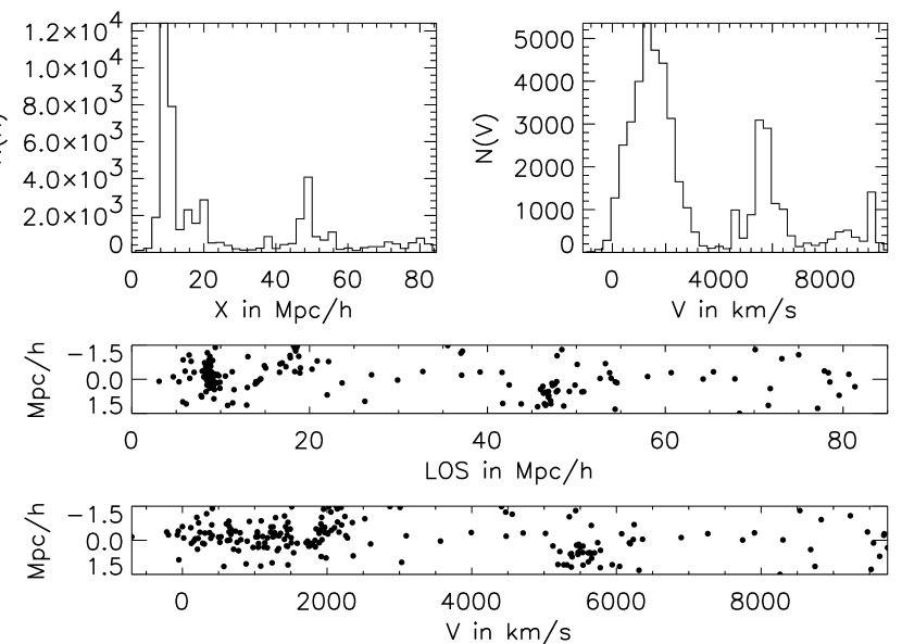
Figure 7: Structure of a moderately contaminated 3-D cluster with $S=4.7$. See the caption of Fig. 6 for a description of the panels.

The cluster in Fig. 7 is a high-mass cluster with $M_{\rm 3-D}=1.5\times 10^{14}\,h^{-1}\,M_{\odot}$, a clump nearby, and a second mass clump $30\,h^{-1}\,$Mpc away. It is detected at $S=4.7$. The velocity dispersion of the projected cluster is broadened from $\sigma_{\rm 3-D}=697\,{\rm km\,s^{-1}}$ to $\sigma_{\rm 2-D}=865\,{\rm km\,s^{-1}}$, and the projected velocity distribution has a bimodal shape. The higher-order moments of the velocity distribution indicate this through skewness and curtosis in projection (${\cal S}_{\rm 2-D}=1.85$ and ${\cal K}_{\rm 2-D}=3.27$), compared to 3-D (${\cal S}_{\rm 3-D}=0.18$ and ${\cal K}_{\rm 3-D}=-0.40$). The cluster satisfies Abell’s criterion with richness class ${\cal R}=0$, both in projection and in 3-D.

4.3 $S$-statistics: $4>S\geq 3$

The last class considered contains clusters with $S$ between 3 and 4. This class is mainly discussed for reasons of completeness. Clusters identified with such signal-to-noise correspond to lower-mass objects making projection effects along the line-of-sight more important. This can be seen looking at the three examples in Fig. 8 and in Figs. 16 and 17.

Figure 8: Line-of-sight structure of a highly contaminated cluster. This cluster is detected at $S=3.2$. See the caption of Fig. 6 for a description of the panels.

The peak with $S=3.2$ corresponding to the cluster shown in Fig. 8 is due to a 3-D cluster with a rather low mass only, $M_{\rm 3-D}=5.9\times 10^{13}\,h^{-1}\,M_{\odot}$. Compared to the low 3-D cluster mass, there is a high amount of intervening matter with several mass clumps along the line-of-sight. Because of this substantial contamination, the projected velocity dispersion is overestimated; $\sigma_{\rm 2-D}=669\,{\rm km\,s^{-1}}$ compared to $\sigma_{\rm 3-D}=364\,{\rm km\,s^{-1}}$ for the 3-D cluster. The velocity histogram has a second peak at the high-velocity tail of the distribution. The higher-order moments of the velocity distribution of the 3-D cluster (${\cal S}_{\rm 3-D}=-0.05$ and ${\cal K}_{\rm 3-D}=-0.07$) change by a large amount when looking at the projected velocity distribution (${\cal S}_{\rm 2-D}=1.12$ and ${\cal K}_{\rm 2-D}=2.43$). This reflects the large influence the intervening matter exerts on observation.

5 Mass estimates

The previous two sections put emphasis on the completeness of catalogues constructed with two different selection criteria, Abell’s criterion and the $S$-statistics based on weak gravitational lensing. Furthermore, we investigated the structure of some detected clusters along the line-of-sight. Of course, both kinds of information are important when deriving statistical information from such catalogues. A third very important test for cosmological theories are the different mass estimates and their relationship with each other. A mass estimate closely related to the optical selection derives from the virial theorem. As a gravitational-lensing based mass estimate, we choose the $\zeta$-statistics, which is closely related to the $S$-statistics as demonstrated in Sect. 2.3.4.

Under the assumption that clusters of galaxies are bound self-gravitating systems in dynamical equilibrium, the total cluster mass can be estimated via the virial theorem (Binney & Tremaine 1987; Sarazin 1986),

$$M_{\rm tot}=\frac{R_{\rm G}\langle v^{2}\rangle}{G}\;,$$ (33)

where $R_{\rm G}$ is the gravitational radius of the cluster relating the system’s mass to its potential energy. Gunn & Gott (1972) showed that this radius is approximately given by $r_{200}$, the radius of a sphere containing an overdensity of $200\,\rho_{\rm crit}$. For the clusters of our study, a radius of $R_{\rm G}=0.75\,h^{-1}\,$Mpc is a good approximation. Observationally, only the los velocity dispersion $\sigma_{\parallel}$ can be measured. Assuming isotropic orbits, the two quantities are related by $\langle v^{2}\rangle=3\sigma_{\parallel}^{2}$.

When calculating the radial velocities from simulated data, the Hubble flow has to be added to the peculiar velocities of the simulation. Since the simulation data are at high redshift, the dependence on redshift of the cosmological constants also has to be taken into account. Therefore, the radial velocities are given by

$$v_{\parallel}=\dot{a}(z)\,x_{\parallel}+a(z)\,\dot{x}_{\parallel}=a(t)\,[H(z)\,x_{\parallel}+\dot{x}_{\parallel}]\;,$$ (34)

with the expansion factor

$$a(z)=(1+z)^{-1}$$ (35)

and the Hubble parameter

$$H(z)=H_{0}\,(1+z)^{3/2}\;.$$ (36)

Apart from the validity of the virial theorem, the virial mass estimate depends solely on a correct estimate of the velocity dispersion $\sigma_{\parallel}$. Since the velocity dispersion is very sensitive to field galaxies and small sub-clumps projected onto the main clusters, it is important to remove these from the sample. We convolve the velocity histogram with a $4000\,{\rm km\,s^{-1}}$ wide top-hat filter to reject interlopers, i.e. galaxies with relative velocities greater than $4000\,{\rm km\,s^{-1}}$ from the peak of the convolved histogram are removed. We further employ the so-called $3\sigma$-clipping procedure proposed by Yahil & Vidal (1977) which has widely been applied to observational samples. It can be summarised as follows:

1. compute the mean radial velocity;

2. remove the galaxy which deviates most from the mean of the sample and re-determine the mean without this galaxy;

3. if the removed galaxy deviates from the new mean by more than $3\sigma$, it is removed from the sample;

4. repeat the procedure until the last tested galaxy remains in the sample.

Figure 9: Comparison of the virial mass estimate $M_{\rm VT}$ to the true cluster mass $M_{\rm 3-D}$. Both panels of this figure display the ratio $M_{\rm VT}/M_{\rm 3-D}$ as a function of the true cluster mass $M_{\rm 3-D}$. In the left panel, the velocity dispersions before $3\sigma$ clipping are used to compute the virial-theorem based mass estimate, while in the right panel, the velocity dispersions after $3\sigma$ clipping are used. In both panels, the open circles refer to ${\cal R}=0$ clusters and the filled circles to ${\cal R}=1$ clusters.

Figure 9 displays the correlation of the virial mass estimate with the true mass of the corresponding 3-D cluster. The left and right panels show the ratio of the virial mass with the 3-D cluster mass as a function of the 3-D mass before and after $3\sigma$ clipping, respectively.

Table 3: Comparison of statistical parameters for the ratio $M_{\rm VT}/M_{\rm 3-D}$ and $M_{\zeta}/M_{\rm 3-D}$ for different sub-samples of masses estimated via the velocity dispersion and the $\zeta$-statistics.

sample	mean	median	standard deviation
complete optical sample before $3\sigma$ clipping	4.90	3.52	1.91
Abell cluster ${\cal R}=1$ before $3\sigma$ clipping	3.84	1.86	1.10
Abell cluster ${\cal R}=0$ before $3\sigma$ clipping	5.44	3.73	2.67
complete optical sample after $3\sigma$ clipping	4.53	3.39	2.01
Abell cluster ${\cal R}=1$ after $3\sigma$ clipping	3.58	1.86	1.18
Abell cluster ${\cal R}=0$ after $3\sigma$ clipping	5.01	3.67	2.80
complete lensing sample	1.27	1.05	0.34
$S\geq 5$	1.23	1.13	0.34
$5\geq S\geq 4$	1.32	1.02	0.31

The first thing to notice is that the masses of clusters with richness class ${\cal R}>0$ are less severely overestimated than masses of clusters with lower richness. This holds true for the mass estimates before and after $3\sigma$-clipping for both the mean and the median, as can be seen in Tab. 3. The second thing readily seen in Fig. 9 and Tab. 3 is the large dispersion of the underlying distribution. This dispersion is smaller for clusters with higher richness class than for clusters with the lowest richness class ${\cal R}=0$ considered. We also note that this dispersion is hardly affected by the $3\sigma$-clipping procedure. The only effect of the clipping procedure is to reduce the average of the estimated cluster masses irrespective of the richness class. A third trend to be seen in Fig. 9 is that the overestimation of the mass is generally more severe for 3-D clusters with lower mass. For the most massive clusters in the sample ($M_{3-D}\lesssim 2.0\times 10^{14}\,h^{-1}\,M_{\odot}$), the continuation of this trend in some cases leads to an underestimation of the masses, as can be seen in the right-hand side of each panel in Fig. 9. The $3\sigma$ clipping procedure fails to correct for the mass overestimates. When comparing Fig. 9 and Tab. 3 to Fig. 15 of Cen (1997), one has to keep in mind the different selection procedure for clusters or groups of galaxies in both studies, but on the whole the results are consistent.

The behaviour described above can largely be attributed to the influence of projection effects on the velocity dispersion. Generally, the inclusion of field galaxies and unvirialised sub-clumps broadens the distribution and leads to distributions which deviate significantly from Gaussian shape, as illustrated by the examples in Sect. 4. The clipping procedure is successful when the amount of contamination along the line-of-sight is low or moderate, but the algorithm fails to remove larger sub-clumps projected onto the main cluster which can significantly broaden the distribution, sometimes even making it bimodal. In some cases it is possible that the clipping procedure removes galaxies belonging to the 3-D cluster, thus contributing to an underestimation of the mass.

Even though we expect from the studies of Frenk et al. (1990) and van Haarlem et al. (1997) that the high-velocity tail of the velocity distribution is severely overestimated, the effect on the mass estimate is most pronounced for galaxy clusters with lower mass. This is due to the fact that they are more easily overestimated with respect to their true dispersion.

Figure 10: Comparison of the $\zeta$-statistics mass estimate to the true cluster mass $M_{\rm 3-D}$. Diamonds and circles refer to clusters identified with a $S\geq 5$ and $S\geq 4$, respectively. Clusters detected at lower $S$ are excluded because of their high contamination.

The $\zeta$-statistics as compared to Abell’s criterion leads to smaller overestimates of the 3-D cluster masses as shown in Fig. 10. Interpreting the quantitative results of the $\zeta$-statistics mass estimate, one has to keep in mind two competing effects: On the one hand, the $\zeta$-statistics, like every gravitational-lensing based method, measures all the mass along the line-of-sight to the cluster; on the other hand, it gives a lower bound to the cluster mass. In combination, these two competing effects lead to fairly moderate mass overestimates, as can be seen in Tab. 3. This also explains the difference to the lensing mass estimates given in the paper by Cen (1997). There, all masses along the line of sight are added up under the assumption of a perfect lensing reconstruction method with an otherwise calibrated mass-sheet degeneracy.

The other interesting feature in Fig. 10 and Tab. 3 is the low dispersion of the underlying distribution. This dispersion does not depend sensitively on the $S$-value at which the clusters are detected. (Clusters detected with $S<4$ where excluded here because of their large contamination.) The dispersion is typically less than a third of the dispersion in the Abell samples.

As for clusters detected with Abell’s criterion, masses of small 3-D clusters are more strongly overestimated than for more massive 3-D clusters. This is due to the fact that the proportion of contaminating matter to the 3-D cluster mass is higher for less massive 3-D objects than for the extremely massive objects. For the intermediate-mass objects, the fact that the $\zeta$-statistics only gives lower bounds to the masses partially outweighs this effect. There, the masses are even slightly underestimated.

Investigating the relationship between velocity-based mass estimates and the gravitational lensing based $\zeta$-statistics in Fig. 11, we see that the $\zeta$-statistics gives on average smaller estimates of the 3-D cluster masses than the virial theorem. Again we stress that this is due to the fact that the $\zeta$-statistics is derived under the assumption of an empty outer annulus, restricting it to estimate lower bounds to the masses. The dispersion between the ratio of $\zeta$-statistics mass to virial mass is large, which is due to the large underlying dispersion in the virial mass estimate.

Figure 11: Comparison of the $\zeta$-statistics mass estimate to the virial mass estimate $M_{\rm VT}$. Only such clusters are included which are detected with both methods, Abell’s criterion and $S$-statistics. Only clusters with $S>4$ are considered.

6 Conclusions

We investigated for the first time with simulated data whether mass-selected galaxy cluster samples are more reliable than samples constructed via Abell’s criterion. Selection of clusters by mass is possible through their gravitational lensing effects, in particular through the coherent image distortion patterns imposed on faint galaxies in their background. As mentioned in the introduction, image distortions trace the gravitational tidal field of a lens rather than its mass, and it is in that sense that we speak of “mass-selected” cluster samples. The second-order aperture-mass statistics $M_{\rm ap}$ was used which is particularly suitable for detecting dark-matter haloes. The signal-to-noise ratio, $S$, of $M_{\rm ap}$ provides a straightforward detection criterion. We also compared the performance of cluster mass estimators based on cluster-galaxy kinematics and gravitational lensing. Our results can be summarised as follows.

1. As already found in previous studies, Abell clusters are severely affected by projection effects. This not only concerns the selection of Abell clusters, but also mass estimates based on galaxy kinematics and the virial theorem, indicating that the velocity dispersion is also hampered by projection effects. A second reason for the failure is the fact that the assumption of dynamical equilibrium is not justified in at least some of the clusters. The projection effects are worse for clusters and groups of lower richness class.

2. Clusters detected with a high significance $S$ of $M_{\rm ap}$ are less affected by projection effects than typical Abell-selected clusters. Like Abell cluster samples, the mass-selected cluster samples are generally incomplete: Samples of clusters detected above a certain $S$ threshold typically do not encompass all three-dimensional clusters present in the simulation; some clusters have lower $S$. However, the completeness of the samples can be increased by lowering the $S$ threshold. We therefore investigated the effect of varying the $S$ threshold on the samples. Completeness of $\approx 100\%$ can be achieved for massive three-dimensional cluster samples ($M\gtrsim 10^{14}\,h^{-1}\,M_{\odot}$) by varying $S\gtrsim 4$. Then, the samples also contain a substantial fraction of spurious detections, most of which correspond to real clusters with smaller masses. Generally, there is a trade-off between completeness and the contamination by spurious detections. More complete cluster samples are more heavily contaminated by spurious clusters, and the balance can be adapted choosing the $S$ threshold. It should be noted that the exact thresholds on $S$ depend somewhat on the choice of the weight function entering the definition of $S$ (cf. the discussion in Sect. 2).

3. While qualitatively the same trend is also observed in Abell-selected cluster samples, the $S$-statistics generally performs significantly better than Abell’s criterion: Higher completeness can typically be achieved with a lower fraction of spurious detections. For instance, cluster samples detected at $S\geq 4$ contain all of the most massive clusters in the simulation and 65% spurious detections, while Abell samples with richness ${\cal R}\geq 0$ encompass only about two-thirds of the most massive clusters and 82% spurious detections.

4. Lensing-based mass estimates are significantly more accurate than mass estimates based on cluster-galaxy kinematics and the virial theorem. Virial masses are typically biased high because line-of-sight velocity distributions are broadened by projection effects. Lensing also adds up mass in front of and behind the clusters, but the bias is less severe. The standard deviation from the true (three-dimensional) mass of the lensing mass estimate is smaller by a factor of three or more than that of the virial mass estimates. It should, however, be noticed that the accuracy of lensing-based mass estimates depends on the depth of the background-galaxy sample and other observational effects. While the mass estimates based on the $\zeta$ statistics are accurate to within $\approx 30\%$ in our simulations, they may well be less accurate under realistic observational conditions.

Our study underestimates projection effects because of the limited size of the simulation volume. This affects both the optical and the lensing-based cluster selection. Yet it appears that selection of clusters by mass yields more reliable cluster samples than optical cluster selection, and, more importantly, the quality of the samples can be controlled by an objective criterion, namely the signal-to-noise threshold imposed.

Selection of clusters by their gravitational-lensing effects is comparable to selection by their X-ray luminosity. In essence, both methods measure weighted projections of the Newtonian cluster potential along the line-of-sight. However, lensing-based cluster detections only require sufficiently deep imaging of wide fields in optical or near-infrared wave bands, and detection algorithms can then be applied in a straightforward manner. In particular, lensing can detect clusters out to significantly higher redshifts than X-ray surveys. What is more, lensing-based mass estimates do not rely on any assumptions on the composition and physical state of the cluster matter, in contrast to X-ray mass estimates. It can therefore be expected that reliable, mass-selected cluster samples at moderate to high redshifts can be constructed in the near future from upcoming deep, wide-field surveys with a straightforward, well-controlled algorithm, and that the accuracy of cluster mass estimates will generally be substantially improved.

Lensing-based cluster detection algorithms like that based on the $S$-statistics can be utilised for cosmology without reference to actual 3-D clusters. Instead, one could define a “cluster” operationally as something visible as a sufficiently high peak in an $S$ map, and then compare model predictions with observations (cf. Kruse & Schneider 1999). If, however, emphasis is laid on clusters as individual entities, it needs to be clarified how well different selection criteria fare in detecting true clusters. Our study has shown that selection of clusters by means of gravitational lensing techniques can be adapted such that the resulting samples are superior to Abell-selected samples in terms of completeness, spurious detections, and the quality of mass estimates.

Appendix A Structure of further representative clusters

We give a few more examples of line-of-sight structures of $S$-selected galaxy clusters here.

A.1 $S$-statistics: $S\geq 5$

A second example for a cluster with high $S$ is given in Fig. 12. The cluster is detected at $S=9.6$. The particle distribution in real space is broad and dominated by a massive 3-D cluster with a mass of $2.1\times 10^{14}\,h^{-1}\,M_{\odot}$. This cluster is detected as an Abell cluster in projection, but the main 3-D cluster by itself already passes the luminosity threshold of a 3-D Abell cluster. In contrast to the first example, the velocity dispersion is hardly affected by projection. The 3-D cluster has a velocity dispersion of $\sigma_{\rm 3-D}=884\,{\rm km\,s^{-1}}$, while the dispersion of the projected cluster is $\sigma_{\rm 2-D}=779\,{\rm km\,s^{-1}}$. The higher-order moments indicate a velocity distribution close to Gaussian shape for both the 3-D cluster (${\cal S}_{\rm 3-D}=0.01$, ${\cal K}_{\rm 3-D}=-0.04$) and the projected cluster (${\cal S}_{\rm 2-D}=0.09$, ${\cal K}_{\rm 2-D}=-0.37$). All this reveals a fairly relaxed cluster with low contamination.

Figure 12: Structure of a massive 3-D cluster detected with $S=9.6$. See the caption of Fig. 6 for a description of the panels.

Almost all other clusters in this class show similar position and velocity histograms. The only exceptions are the 2-D clusters corresponding to less massive 3-D clusters. For one of these clusters with relatively high $S=7.9$, the structure is given in Fig. 13. Even though the position histogram is dominated by a 3-D cluster, the distribution for this cluster is broad, and there is a large amount of intervening matter with at least four smaller clumps with masses of order $M=10^{13}\,h^{-1}\,M_{\odot}$. Qualitatively, the los velocity histogram looks artificially broadened by these clumps, and in fact the velocity dispersion ($\sigma_{\rm 3-D}=651\,{\rm km\,s^{-1}}$) is significantly increased in projection ($\sigma_{\rm 2-D}=860\,{\rm km\,s^{-1}}$). The higher-order moments are also strongly affected by this intervening matter (${\cal S}_{\rm 3-D}=-0.05$ and ${\cal K}_{\rm 3-D}=-0.64$ compared to ${\cal S}_{\rm 2-D}=1.19$ and ${\cal K}_{\rm 2-D}=0.87$). This cluster is detected as ${\cal R}=1$ Abell cluster although it corresponds only to a ${\cal R}=0$ cluster in 3-D.

Figure 13: Structure of a less massive 3-D cluster whose size is increased in projection due to matter concentrations along the line-of-sight. See the caption of Fig. 6 for a description of the panels.

A.2 $S$-statistics: $5>S\geq 4$

Figure 14: Structure of a moderately contaminated 3-D cluster with a $S=4.7$. See the caption of Fig. 6 for a description of the panels.

Figure 14 shows a cluster with $S=4.7$. It is apparently only mildly contaminated by a clump $30\,h^{-1}\,$Mpc from the main clump, which is a high-mass object with $M_{\rm 3-D}=2.3\times 10^{14}\,h^{-1}\,M_{\odot}$. The projected velocity dispersion is almost unaffected ($\sigma_{\rm 2-D}=650\,{\rm km\,s^{-1}}$ compared to $\sigma_{\rm 3-D}=635\,{\rm km\,s^{-1}}$), and shows a bimodal feature, which is also reflected by the curtosis of the projected cluster, ${\cal K}_{\rm 2-D}=0.51$, while the velocity distribution of the 3-D cluster has a negative curtosis of ${\cal K}_{\rm 3-D}=-0.22$. Similarly, the skewness changes from ${\cal S}_{\rm 2-D}=-0.44$ to ${\cal S}_{\rm 3-D}=-0.03$. The cluster is detected as a 2-D Abell cluster with richness class ${\cal R}=1$, while the richness class of the 3-D cluster is ${\cal R}=0$. Therefore, the richness class is inflated due to projection. Even though this cluster shows some projection effects, the corresponding 3-D cluster is massive and therefore clusters like that should be included in a mass-limited sample.

Figure 15: Structure of a moderately contaminated 3-D cluster with $S=4.4$. See the caption of Fig. 6 for a description of the panels.

The last example for this class is shown in Fig. 15. Here, the $S$-map has a peak with $S=4.4$. The position histogram shows a very broad peak with a secondary maximum on top of the main peak. The corresponding 3-D cluster has a high mass, $M_{\rm 3-D}=3.4\times 10^{14}\,h^{-1}\,M_{\odot}$. The projected velocity distribution is only moderately skewed with ${\cal S}_{\rm 2-D}=0.22$ compared to the skewness of the main cluster alone, ${\cal S}_{\rm 3-D}=0.17$. However, the curtosis of the projected peak, ${\cal K}_{\rm 2-D}=0.38$, even changes sign when compared to the 3-D cluster, ${\cal K}_{\rm 3-D}=-0.27$. This cluster satisfies Abell’s criterion in projection, but the main peak has a lower richness class, ${\cal R}=0$.

A.3 $S$-statistics: $4>S\geq 3$

Figure 16: Structure of moderately large 3-D group with $S$ between 3 and 4. The 3-D object is contaminated by projection along the line-of-sight, leading to an increased $S$ of $3.4$. See the caption of Fig. 6 for a description of the panels.

Another example for a low-$S$ cluster detected at $S=3.4$ is displayed in Fig. 16. This detection also corresponds to a 3-D cluster with $M_{\rm 3-D}=6.6\times 10^{13}\,h^{-1}\,M_{\odot}$. Again, the velocity distribution of this cluster is largely altered by the considerable amount of intervening matter. The velocity dispersion itself is inflated from $\sigma_{\rm 3-D}=504\,{\rm km\,s^{-1}}$ to $\sigma_{\rm 2-D}=1134\,{\rm km\,s^{-1}}$. This is reflected by the curtosis, which changes from ${\cal K}_{\rm 3-D}=-0.02$ to ${\cal K}_{\rm 2-D}=-0.5$, while the skewness changes from ${\cal S}_{\rm 3-D}=0.18$ to ${\cal S}_{\rm 2-D}=-0.94$. Both low-$S$ examples are neither 2-D Abell clusters nor do they pass the selection criteria for Abell clusters in 3-D.

Figure 17: Structure of a spuriously detected object which does not correspond to a 3-D cluster. The high contamination along the line-of-sight leads to $S=3.8$. See the caption of Fig. 6 for a description of the panels.

The last example in Fig. 17 with $S=3.75$ does not correspond to a 3-D cluster or group with mass exceeding $M_{\rm 3-D}=10^{13}\,h^{-1}\,M_{\odot}$. Instead, one sees a large amount of contaminating matter and smaller sub-clumps. This material is responsible for the signal in the $S$ map. The velocity distribution is characterised by three peaks with dispersion $\sigma_{\rm 2-D}=1235\,{\rm km\,s^{-1}}$, skewness ${\cal S}_{\rm 2-D}=-0.30$, and curtosis ${\cal K}_{\rm 2-D}=-1.39$. Obviously, the contamination along the line-of-sight is large enough to lead to the detection of an Abell cluster with richness class ${\cal R}=0$.

References

- [1] Abell G.O., 1958, ApJS, 3, 211
- [2] Bartelmann, M., 1995, A&A, 303, 643
- [3] Bartelmann M., Narayan R., 1995, ApJ, 451, 60
- [4] Bartelmann M., Steinmetz, M., 1996, MNRAS, 283, 431
- [5] Bartelmann M., Narayan, R., Seitz, S., Schneider, P., 1996, ApJ, 464, L115
- [6] Binney J., Tremaine S., 1987, Galactic Dynamics, Princeton University Press
- [7] Bond J.R., Efstathiou G., 1984, ApJ, 285, L45
- [8] Cen R., 1997, ApJ, 485, 39
- [9] Cole S.M., Lacey C., 1996, MNRAS, 281, 716
- [10] Couchman H.M.P., Thomas P.A., Pearce F.R., 1995, ApJ, 452, 797
- [11] Couchman H.M.P., Thomas P.A., Pearce F.R., 1996, astro-ph/9603116
- [12] Davis M., Efstathiou G.P., Frenk C.S., White S.D.M., 1985, ApJ, 292, 371
- [13] Fahlman G., Kaiser N., Squires G., Woods D., 1994, ApJ, 437, 56
- [14] Frenk C.S., White S.D.M., Efstathiou G., Davis M., 1990, ApJ, 351, 10
- [15] Gunn J., Gott J.R., 1972, ApJ, 176, 1
- [16] Jenkins A., Frenk, C.S., Pearce, F.R., Thomas, P.A., et al., 1998, ApJ, 499, 20
- [17] Kaiser N., 1995, ApJ, 439, L1
- [18] Kaiser, N., Squires, G., 1993, ApJ, 404, 441
- [19] Kaiser, N., Squires, G., Broadhurst, T., 1995, ApJ, 449, 460
- [20] Kaiser, N., Wilson, G., Luppino, G., Kofman, L., Gioia, I., Metzger, M., Dahle, H., 1998, ApJ submitted, preprint astro-ph/9809268
- [21] Kauffmann, G.A.M., Colberg, J.M., Diaferio, A., White, S.D.M., MNRAS submitted, preprint astro-ph/9805283
- [22] Kruse, G., Schneider, P., 1999, MNRAS, 302, 821
- [23] Lucey J.R., 1983, MNRAS, 204, 33
- [24] Marzke R.O., Huchra J.P., Geller M.J., 1994, ApJ, 428, 43
- [25] Sarazin C.L., 1986, Rev. Mod. Phys., 58, 1
- [26] Schechter P., 1976, ApJ, 203, 297
- [27] Schneider P., 1996, MNRAS, 283, 837
- [28] Schneider P., Kneib J.P., in: The Next Generation Space Telescope: Science Drivers and Technological Challenges, 34th Liège Astrophysics Colloquium, June 1998, p. 89
- [29] Schneider P., Seitz C., 1995, A&A, 294, 411
- [30] Schneider P., Ehlers J., Falco E.E., 1992, Gravitational Lenses, Springer-Verlag
- [31] Schramm T., Kayser R., 1995, A&A, 299, 1
- [32] Seitz C., Schneider P., 1995, A&A, 297, 287
- [33] Seitz C., Schneider P., 1997, A&A, 318, 687
- [34] Seitz, S., Schneider, P., 1996, A&A, 305, 383
- [35] Squires, G., Kaiser, N., 1996, ApJ, 473, 65
- [36] Swarztrauber P., 1984, in Golub G., ed., Studies in Numerical Analysis, 24, p.319
- [37] van Haarlem M.P., Frenk C.S., White S.D.M., 1997, MNRAS, 287, 817
- [38] White S.D.M., Efstathiou G., Frenk C.S., 1993, MNRAS, 262, 1023
- [39] Yahil A., Vidal N.V., 1977, ApJ, 214, 347