Vorticity generation in large-scale structure caustics

Abstract

A fundamental hypothesis for the interpretation of the measured large-scale line-of-sight peculiar velocities of galaxies is that the large-scale cosmic flows are irrotational. In order to assess the validity of this assumption, we estimate, within the frame of the gravitational instability scenario, the amount of vorticity generated after the first shell crossings in large-scale caustics. In the Zel’dovich approximation the first emerging singularities form sheet like structures. Here we compute the expectation profile of an initial overdensity under the constraint that it goes through its first shell crossing at the present time. We find that this profile corresponds to rather oblate structures in Lagrangian space. Assuming the Zel’dovich approximation is still adequate not only at the first stages of the evolution but also slightly after the first shell crossing, we calculate the size and shape of those caustics and their vorticity content as a function of time and for different cosmologies.

The average vorticity created in these caustics is small: of the order of one (in units of the Hubble constant). To illustrate this point we compute the contribution of such caustics to the probability distribution function of the filtered vorticity at large scales. We find that this contribution that this yields a negligible contribution at the 10 to 15 $h^{-1}$Mpc scales. It becomes significant only at the scales of 3 to 4 $h^{-1}$Mpc, that is, slightly above the galaxy cluster scales.

1 Introduction

The analysis of large-scale cosmic flows has become a very active field in cosmology (see Dekel 1994 for a recent review on the subject). The main reason is that it can in principle give access to direct dynamical measurements of various quantities of cosmological interest. There are now a very large number of methods and results for the comparison of the measured large–scale flows with the measured density fluctuations as observed in the galaxy catalogues. Most of these methods are sensitive to a combination of the density of the universe in units of the critical density, $\Omega$, and the linear bias, $b$, associated to the mass tracers adopted to estimate the density fluctuations. The estimated values of $\beta=\Omega^{0.6}/b$ are about $0.3$ to 1 depending on the method or on the tracers that are used. There are other lines of activities that aim to estimate $\Omega$ from only the intrinsic properties of the velocity field, (i.e., without comparison with the observed galaxy density fluctuations). All these methods exploit non-Gaussian features expected to appear in the velocity field, either the maximum expansion rate of the voids (Dekel & Rees 1994), non-Gaussian general features as expected from the Zel’dovich approximation (Nusser & Dekel 1993), or the skewness of the velocity divergence distribution (Bernardeau et al. 1995). Yet they all also assume that the velocity field is potential. This is indeed a necessary requirement for building the whole 3D velocity out of the line-of-sight informations in reconstruction schemes such as Potent (Bertschinger & al. 1990, Dekel et al. 1994). This is also a required assumption for carrying calculations in the framework of perturbation theory. It is therefore interesting to check the rotational content of the cosmic flows at scales at which they are considered in galaxy catalogues, that is at about 10 to 15$h^{-1}$Mpc. This investigation ought to be carried in the frame of the gravitational instability scenario with Gaussian initial conditions. It is known that in the single stream régime, primordial vorticity is diluted by the expansion and that the higher order terms in a perturbation expansion cannot create “new” vorticity. Hence it is natural to assume that the vorticity on larger scales originate from the (rare) regions where multi-streaming occurs. During the formation of large scale structures this happens first when the largest caustics cross the first singularity, creating a three-flow region where vorticity can be generated. As we argue in Sect. 2, analytical calculations of constrained random Gaussian fields suggest that the largest caustics that are created are sheet-like structures, in rough agreement with what is found in numerical simulations or in galaxy catalogues. It is therefore reasonable to use Zel’dovich’s approximation to describe the subsequent evolution of those objects.

In order to estimate the large scales vorticity distribution we therefore proceed in five steps: first we evaluate the mean constrained random field corresponding to a local asymmetry of the deformation tensor on a given scale, $R_{L}$; secondly we solve for the multi-flow régime within the generated caustic, using Zel’dovich’s approximation throughout, even slightly beyond this first singularity. We then evaluate the vorticity field in that caustic. The next step involves modelling the variation of the characteristics of typical caustics as a function of time for different power spectra. Finally, we estimate the amount of vorticity expected at large scales arising from large scale flow caustics.

For the sake of simplicity and because is pedagologically more appealing, we present calculations carried out in two dimensions as well as in three dimensions. The former case is in particular easier to handle numerically.

The second Section of this paper evaluates the characteristics of the typical caustics expected at large–scale in a 2D or 3D density field. The third Section is devoted to the explicit calculation of the vorticity for the most typical caustics. The fourth Section provides an estimate for the shape of the tail of the probability distribution function of the modulus of the vorticity in a sphere of a given radius. It is followed by a discussion on the validity and implications of these results.

2 Asymmetric constrained random fields

Since it is not our ambition to solve the problem of deriving the vorticity statistics in its whole generality the vorticity will be estimated only within specific but typical caustics in the framework of the Zel’dovich approximation.

The first step involves building an initial density field in which a caustic will eventually appear. The initial fluctuations are assumed to be Gaussian with a given power spectrum $P(k)$, characterizing the amplitude and shape of the initial fluctuations. No a priori assumptions about the values of $\Omega$ and $\Lambda$ are made. It will be shown that the statistics has very straightforward dependences upon these parameters. The expectation values of the random variables, $\delta({\bf k})$, corresponding to the Fourier transforms of the local density field,

$$\delta({\bf x})=\int{\rm d}^{3}{\bf k}\,\delta({\bf k})\,\exp[{\rm i}{\bf k}\cdot{\bf x}],$$ (1)

are calculated once a local constraint has been imposed. This constraint will be chosen so that the caustic-to-be will have just gone through first shell crossing at the present time. It is expressed in terms of the local deformation matrix of the smoothed density field. The components of the local deformation tensor at the position ${\bf x}_{0}$ are given by

$$\Phi_{i,j}({\bf x}_{0})=\int{\rm d}^{3}{\bf k}\ \delta({\bf k})\ W_{D}(k\,R_{L})\exp[{\rm i}{\bf k}\cdot{\bf x}_{0}]\,{{\bf k}_{i}{\bf k}_{j}\over k^{2}},$$ (2)

where $W_{D}$ is the adopted window function. In what follows, we will use the top-hat window function for which

$$W_{2}(k)=2\ {J_{1}(k)\over k^{1/2}}\quad{\rm in\ }\ \ 2D,\ \ W_{3}(k)=3\sqrt{\pi/2}\ {J_{3/2}(k)\over k^{3/2}}\ \ {\rm in\ }\ \ 3D,$$ (3)

where $J_{\nu}$ is the Bessel function of index $\nu$. The scale $R_{L}$ is the scale of the caustic in Lagrangian space. Here $\sigma_{0}$ stands for the rms density fluctuation at this scale:

$$\sigma_{0}^{2}=\int{\rm d}^{3}k\,P(k)\,W_{2}^{2}(k\,R_{L}).$$ (4)

For the sake of simplicity a typical caustic is chosen to be characterized by the average local perturbation over a sphere of radius $R_{L}$ for which the deformation tensor at its centre is fixed. We are aware that this is a somewhat drastic approximation but consider that, at large scales, the behaviour of caustics having the mean initial profile will be representative of the average behaviour. This is certainly not true at small scales where the complex interactions of structures at different scales and positions are expected to affect the global behaviour of any given caustic. For some rare enough objects however we expect the fluctuations around the mean profile to be small enough to affect only weakly the global properties of the caustics. This has been shown to be true in the early stages of the dynamics for spherically symmetric perturbations (Bernardeau 1994a). In the following we will, however, encounter properties (see §3.3) that we think are not robust against small scale fluctuations. Such properties will be ignored in the subsequent applications of our results.

Within the frame of this calculation, the values of $\delta({\bf k})$ hence correspond to the expectation values of $\delta({\bf k})$ for the power spectrum $P(k)$ when the constraints on the deformation tensor are satisfied. These solutions can be written as a linear combination of the values of the deformation tensor:

$$\delta({\bf k})=\sum_{i=1}^{D}-{\left(C^{-1}\right)_{0,i}\over\left(C^{-1}\right)_{0,0}}\ \lambda_{i}\,\equiv\sum_{i=1}^{D}\,\,\alpha_{i}\,\lambda_{i}\,,$$ (5)

where the coefficients $C$ is the matrix of the cross-correlations between the random Gaussian variables $\Phi_{ij}$ and $\delta({\bf k})$ as shown in Appendix A. In Eq. (5) the summation is made only on the diagonal elements of the deformation tensor since it is always possible to choose the axis in such a way that the other elements are zero. In this instance, the diagonal elements are identified with the eigenvalues $\lambda_{i}$, of the matrix.

2.1 The 2D field

In 2D geometry, the two coefficients $\alpha_{1}$ and $\alpha_{2}$ defined by Eq. (5) are given by

$$\alpha_{1}=(3I_{1}-I_{2})/\sigma_{0}^{2}\,,\ \ \alpha_{2}=(3I_{2}-I_{1})/\sigma_{0}^{2}\,,\ \ {\rm where}\ \ I_{i}=\big{<}\delta_{k}\,\Phi_{ii}\big{>}=P(k)\,W_{2}(kR_{L})\,{{\bf k}_{i}^{2}\over k^{2}}.$$ (6)

The brackets, $\big{<}.\big{>}$, denote ensemble averages over the initial (unconstrained) random density field. As a result, Eq. (5) reads

$$\delta({\bf k})={P(k)\,W_{2}(kR_{L})\over\sigma_{0}^{2}}\,\big{[}2\,(\lambda_{1}+\lambda_{2})+4\,(\lambda_{1}-\lambda_{2})\,\cos(2\theta)\big{]}\,;$$ (7)

$\lambda_{1}$ and $\lambda_{2}$ are the eigenvalues of the deformation tensor and where $\theta$ is the angle between ${\bf k}$ and the eigenvector associated with the first eigenvalue (see Appendix A for details). Consider the parameter $a$ defined by

$$a={2(\lambda_{1}-\lambda_{2})\over\lambda_{1}+\lambda_{2}}.$$ (8)

The coefficient $a$ represents the amount of asymmetry in the fluctuation (thus $a=0$ corresponds to a spherically symmetric perturbation). This parameter is similar to the eccentricity, $e$, that was used by Bardeen et al. (1986) and more specifically by Bond & Efstathiou (1987) for 2D fields. In these studies however investigations were made for the shape of the peaks around the maximum (i.e. eigenvalues of the second order derivatives of the local density), so $a$ and $e$ cannot be straightforwardly identified.

Figure 1: The distribution function of $\lambda_{\rm max}/\sigma_{0}$ (solid line) in 2D dynamics. The dashed line is given by (Eq. (11)):

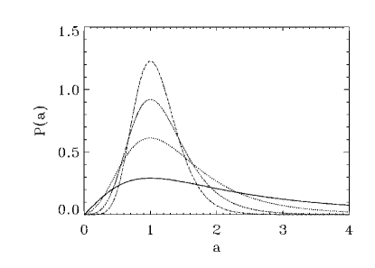
Figure 2: The distribution functions of $a$ for fixed values of $\lambda_{\rm max}/\sigma_{0}=1,\ 2,\ 3,\ 4$ (respectively the solid, long dashed, short dashed and long dotted dashed lines).

The formation time of the first singularity is determined by the maximum value of the eigenvalues, $\lambda_{\rm max}$. It is therefore relevant to calculate the distribution function of $\lambda_{\rm max}$, and the distribution function of $a$ once $\lambda_{\rm max}$ is known. From the statistical properties of the matrix elements $\Phi_{ij}$ we derive the distribution function of the eigenvalues $\lambda_{\rm min}$ and $\lambda_{\rm max}$ (see Appendix B), which reads

$$P(\lambda_{\rm min},\lambda_{\rm max}) = {2^{3/2}\over\pi^{1/2}\,\sigma_{0}^{3}}\,(\lambda_{\rm max}-\lambda_{\rm min})\exp\left[-{1\over\sigma_{0}^{2}}\left({3\over 2}J_{1}^{2}-{4}\,J_{2}\right)\right],$$ (9)

with

$$J_{1}=\lambda_{\rm min}+\lambda_{\rm max}\,,\quad J_{2}=\lambda_{\rm min}\,\lambda_{\rm max}.$$ (10)

The distribution function of $\lambda_{\rm max}$ follows by numerical integration over $\lambda_{\rm min}$. Fig. (2) shows the distribution function of $\lambda_{\rm max}$ in units of the variance. The dashed line corresponds to the approximation, valid at $\lambda_{\rm max}/\sigma_{0}\gg 1$:

$$p_{\rm max}(\lambda_{\rm max})\,{\rm d}\lambda_{\rm max}\approx 1.5\,{\lambda_{\rm max}\over\sigma_{0}}\exp\left[-{4\over 3}\left({\lambda_{\rm max}\over\sigma_{0}}\right)^{2}\right]\ {{\rm d}\lambda_{\rm max}\over\sigma_{0}}.$$ (11)

The distribution function of $a$ for different values of $\lambda_{\rm max}/\sigma_{0}$ is presented in Fig. (2). It turns out that the most significant value corresponds to $a\approx 1$. In the following this value is chosen as the typical value for the asymmetry in two dimensions.

2.2 The 3D field

In three dimensions the geometry is slightly more complicated and yields for the constrained density field (see Appendix B for details)

$$\delta({\bf k}) = {3\ P(k)\,W_{3}(k\,R_{L})\over 8\sigma_{0}^{2}}\ \Big{(}\lambda_{1}\,\big{[}1+5\,\cos(2\phi_{k})-5\cos(2\theta_{k})-5\,\cos(2\phi_{k})\,\cos(2\theta_{k})\big{]}+$$ (12)

$$\lambda_{2}\,\big{[}1+5\,\cos(2\phi_{k})-5\cos(2\theta_{k})-5\,\cos(2\phi_{k})\,\cos(2\theta_{k})\big{]}+\,2\lambda_{3}\,\big{[}3+5\,\cos(2\,\theta_{k})\big{]}\Big{)},$$

where $\theta_{k}$ and $\phi_{k}$ are polar angles of the vector ${\bf k}$ with respect to the basis of the eigenvectors associated to the three eigenvalues, $\lambda_{1},\lambda_{2},\lambda_{3}$. The asymmetry of the distribution is again characterized by the values of

$$a=5\,{2\lambda_{3}-\lambda_{1}-\lambda_{2}\over\lambda_{1}+\lambda_{2}+6\lambda_{3}}\,,\ \ {\rm and}\ \ b=5\,{\lambda_{1}-\lambda_{2}\over\lambda_{1}+\lambda_{2}+6\lambda_{3}}.$$ (13)

When $b$ only is zero Eq. (13) corresponds to a perturbation with axial symmetry, and when both $a$ and $b$ are zero it is a spherically symmetric perturbation. In terms of $a$ and $b$ Eq. (12) then becomes

$$\delta({\bf k})={3\,P(k)\,W_{3}(k\,R_{L})\over 8\,\sigma_{0}^{2}}\,(\lambda_{1}+\lambda_{2}+6\lambda_{3})\Big{(}1+a\,\cos(2\theta_{k})+b\,\cos(2\phi_{k})\big{[}1+\cos(2\theta_{k})\big{]}\Big{)}.$$ (14)

Let us now evaluate the distribution of $a$ and $b$ from the distribution function of the eigenvalues $(\lambda_{1},\lambda_{2},\lambda_{3})$ in 3D (assuming $\lambda_{1}>\lambda_{2}>\lambda_{3}$) in order to identify the shape of the most significant caustics. This distribution is given by (Doroshkevich 1970)

$$P(\lambda_{1},\lambda_{2},\lambda_{3})={5^{5/2}\ 27\over 8\,\pi\,\sigma_{0}^{6}}\,(\lambda_{1}-\lambda_{2})\,(\lambda_{1}-\lambda_{3})\,(\lambda_{2}-\lambda_{3})\,\exp\left[-{1\over\sigma_{0}^{2}}\left(3J_{1}^{2}-{15\over 2}\,J_{2}\right)\right],$$ (15)

with

$$J_{1}=\lambda_{1}+\lambda_{2}+\lambda_{3}\,,\ \ {\rm and}\ \ J_{2}=\lambda_{1}\lambda_{2}+\lambda_{2}\lambda_{3}+\lambda_{3}\lambda_{1}.$$ (16)

From this expression we compute numerically the distribution function of the maximum eigenvalue (Fig. (4)). An analytical fit of this distribution function is provided by its behaviour at large $\lambda_{\rm max}$

$$p_{\rm max}(\lambda_{\rm max})\,{\rm d}\lambda_{\rm max}\approx 6\,\left(\lambda_{\rm max}\over\sigma_{0}\right)^{2}\,\exp\left[-{5\over 2}\left({\lambda_{\rm max}\over\sigma_{0}}\right)^{2}\right]\,{{\rm d}\lambda_{\rm max}\over\sigma_{0}}.$$ (17)

This fit is accurate for the rare event tail (as shown in Fig. (4)), which will be relevant for the derivation of Sect. 4.4. For a given value of $\lambda_{\rm max}$ we compute the distribution of the other eigenvalues, and thus the join distribution function of $a$ and $b$.

Figure 3: The distribution function of $\lambda_{\rm max}/\sigma_{0}$ (solid line) in 3D dynamics. The dashed line is the analytical fit (17).

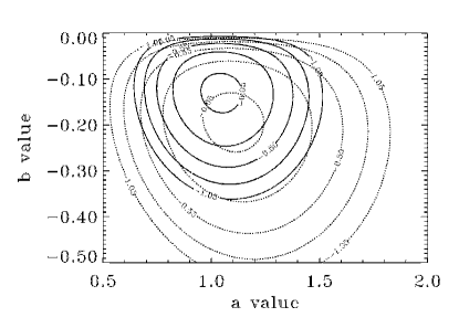
Figure 4: The contour plot for the distribution of $a$ and $b$ for a fixed value of $\lambda_{\rm max}/\sigma_{0}=2$ (dashed lines) and $\lambda_{\rm max}/\sigma_{0}=3$ (solid lines). The lines are evenly distributed in a logarithmic scale.

The resulting contour plot corresponding to $\lambda_{\rm max}/\sigma_{0}=2$ and $\lambda_{\rm max}/\sigma_{0}=3$ is illustrated on Fig. (4). As for the distribution of $a$ in the previous subsection in 2D it depends only weakly upon the adopted value of $\lambda_{\rm max}$ (although the position of the maximum varies a little), and it tends to be all the more peaked on its maximum as $\lambda_{\rm max}$ is large. This implies that a typical caustic will be given by $a\approx 1$ with a small $b$. For further simplifications we will assume that $b=0$. Such a caustic then corresponds to a pancake-like structure with axial symmetry. Note that this result seems to differ from the results of Bardeen et al. (1986) who found that the shape of the rare peaks should be somewhat spherically symmetric or filamentary (this picture was recently sustained by Pogosyan & al., 1996, from the result of $N$-body simulations). This apparent discrepancy is due to the constraint under which the expectation values of $a$ and $b$ are calculated. In Bardeen et al.’s work the constraint is given by the value of the local density, i.e. the sum of the three eigenvalues, whereas in this paper we put a constraint on the largest eigenvalue. This is a natural assumption for this investigation since the multi-streaming occurs as soon as a singularity has been reached in one direction. Of course, this analysis assumes that the Zel’dovich approximation holds in order to predict the time at which this first singularity is reached. For oblate initial structures such as the ones obtained for the most likely values of $a$ (see Figs. 5 and 6), we expect that this approximation is sufficiently accurate.

3 The geometry & vorticity of large-scale caustics

In this section we investigate the properties of the caustics that are induced by the initial density fluctuation profiles we found in the previous section. All the calculations are performed within the framework of the Zel’dovich approximation, even sightly after the first shell crossing.

3.1 The linear displacement field

In the framework of the Zel’dovich approximation the displacement field can be written

$${\bf x}={\bf q}+D(t)/D(t_{0})\,\Psi({\bf q})\,;$$ (18)

where $D(t)$ accounts for the time dependency of the linear growing mode (it is proportional to the expansion factor in case of an Einstein-de Sitter geometry only). An important simplification is that, at the order of the Zel’dovich approximation, this displacement field is separable in time and space, and its space dependence, $\Psi({\bf q})$, is potential, i.e., there is a velocity potential $U({\bf q})$ so that

$$\Psi({\bf q})=\nabla_{{\bf q}}\cdot U({\bf q})\,.$$ (19)

This velocity potential is given by

$$U({\bf q})=\int{\rm d}^{3}{\bf q}\,\delta({\bf k})\,{1\over k^{2}}\,\exp[{\rm i}{\bf k}\cdot({\bf q}-{\bf q}_{0})]\,.$$ (20)

By construction the point ${\bf q}_{0}$ in Lagrangian space corresponds to the point ${\bf x}_{0}$ in real space (central position of the caustic). Both of them will be taken to be zero. For the calculation of the explicit expressions of $\delta({\bf k})$ and $U({\bf q})$ we will assume that the power spectrum follows a power law behaviour,

$$P(k)\propto k^{n},$$ (21)

characterized by the power index $n$. From Eq. (21) the expression of the linear variance as a function of scale follows

$$\sigma(R_{L})\propto R_{L}^{-(n+D)/2}.$$ (22)

This approximation is valid within a limited scale range as will be discussed in Sect. 5. At the scales of interest the index $n$ is expected to be the range of $n\approx-1,\ -2$ from the constraints obtained with the large-scale galaxy catalogues, like the APM survey (Peacock 1991) the IRAS galaxy survey (Fisher et al. 1993) or from X-ray cluster number counts (Henry & Arnaud 1991, Eke et al. 1996, Oukbir & Blanchard 1997). In two dimensions there are of course no such observationally motivated values, but we will consider $n$ of the order of $-1$ as an illustrative case.

3.1.1 The 2D potential

From the Eqs. (7), (20) it is possible to calculate the expression of the potential

$$U({\bf q})=G(0,n-2,q)+a\,\cos(2\theta_{q})\,\left[G(0,n-2,q)-2\ G(1,n-2,q)\right]\,,\quad{\rm with}\quad G(\nu,n,q)=\int{\rm d}^{2}{\bf k}\,k^{n}\,{J_{\nu}(k\,q)\over(k\,q)^{\nu}}\,W_{2D}(k).$$ (23)

The latter expression is given by

$$G(\nu,n,q)=\,_{2}F_{1}(1+n/2,n/2,1+\nu,q^{2})\,,\quad{\rm for}\quad q<1\,,\quad{\rm and}$$ (24)

$$G(\nu,n,q)={\Gamma(1+\nu)\,\Gamma(1-n/2)\over q^{n+2}\,\Gamma(\nu-n/2)}\ \,_{2}F_{1}(1+n/2,1-\nu+n/2,2,q^{-2})\,,\ \ {\rm for}\ \ q>1.$$ (25)

The expressions for the gradients of the potential involve similar hyper-geometric functions.

3.1.2 The 3D potential

The expression of the potential following from Eqs. (12), (20) becomes quite complicated, but involves here only “simple” functions. It reads

$$U({\bf q})=[V(q)-V(-q)]/q^{3},$$ (26)

with

$$V(q) = |1+q|^{2-n}\,{\rm sign}(1+q)\Big{(}{{{\it A}(q)-{\it B}(q)\,\big{[}b\,\cos(2\,\phi)\,\left[1-\cos(2\,\theta)\right]+a\,\cos(2\,\theta)\big{]}}}\Big{)}\,,$$ (27)

$$A(q) = -10\,{q^{2}}+7\,n\,{q^{2}}-{n^{2}}\,{q^{2}}+5\,{q^{3}}-n\,{q^{3}}+a\,\left(-1+2\,q-n\,q+2\,{q^{2}}-n\,{q^{2}}-{q^{3}}\right)\,,$$ (28)

$$B(q) = 3-6\,q+3\,n\,q+4\,{q^{2}}-4\,n\,{q^{2}}+{n^{2}}\,{q^{2}}-2\,{q^{3}}+n\,{q^{3}}$$ (29)

Note that the potentials in Eqs. (23) and  (26) have discontinuous derivative at $q=1$, which is an artifact of using a top-hat window function. Note also that the potentials given here have arbitrary normalizations. This is of no consequence for the derived results since the global normalization of the initial density profile is absorbed in the discussion for the value of $\lambda_{\rm max}$ (Sect. 4.4).

3.2 The shape of the caustics

A multi-flow region forms as soon as Eq. (18) has more than one solution. The corresponding region forms the so-called caustic. These regions are illustrated in Figs. (6) and  (6) in respectively 2 and 3 dimensions for typical values of the parameters. The solid lines show in 2D the shape of the caustic in real space, and the dashed lines their shape in the original Lagrangian space.

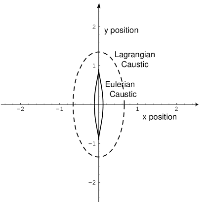
Figure 5: The shape of the caustic for the 2D dynamics, $n=-1$, and $\lambda_{\rm max}\approx 1.3$. The dashed line is the shape in Lagrangian space and the solid line the shape in real space.

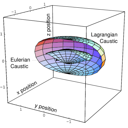
Figure 6: The shape of the caustic for the 3D dynamics, $n=-1.5$ and $\lambda_{\rm max}\approx 1.5$. The external shell is the Lagrangian position of the caustic, the internal one its position in real space.

For the chosen values of $a$ and $b$ and for the relevant $\lambda_{\rm max}$ the caustics form elongated structures. These figures are plotted in units of the smoothing scale $R_{L}$. They suggest that the largest dimension of the caustics are roughly of the order of magnitude of the initial Lagrangian scale. Note that the boundaries of the caustics correspond to surfaces (or lines in 2D) where the Jacobian of the transformation between Lagrangian space and real space vanishes, i.e.

$$J({\bf q})=\big{|}{\partial{\bf x}\over\partial{\bf q}}\big{|}=0.$$ (30)

The size and shape of these caustics are characterized, in 2D and 3D (although only approximately), by two lengths, the half-depth of the caustic, $d$, (that is the distance that has been covered by the shock front after the first singularity) and its half-extension $e$. For instance in Fig. (6) the value of $d$ is about $0.1$ and the value of $e$ is about $0.9$ in units of the Lagrangian size of the fluctuation $R_{L}$. In the case of the 3D dynamics $e$ corresponds to the radius of the caustic since we restrict ourselves to cylindrical symmetry.

The density in each flow “$s$” is given by the inverse of the Jacobian of the transformation so that

$$\rho({\bf q}_{s})=1/J({\bf q}_{s})\,.$$ (31)

The total density within the caustic is then given by the summation over each flow of each of their densities,

$$\rho({\bf x})=\sum_{{\rm flow}\ s}\ \rho({\bf q}_{s}).$$ (32)

3.3 The velocity field, and the generated vorticity

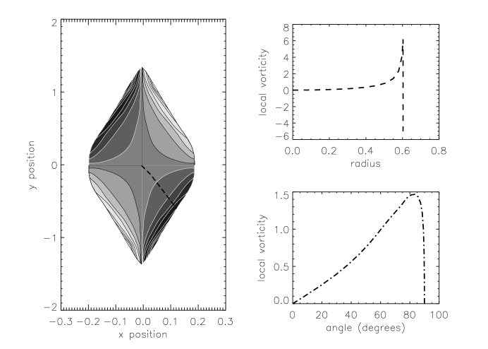
Figure 7: The map of the vorticity in a typical 2D caustic ($n=-1$). Left panel: the local vorticity is antisymmetric with respect to the centre of the caustic. It points along the Z-axis, and is positive in the second and fourth quadrant, and negative in the first and third. Right panels: behavior of the local vorticity along two different lines (thick dot-dashed line on the left panel). The top panel shows that the vorticity is singular near the edge of the caustic. It behaves as described by Eq. (43) and there is a non zero lineic vorticity located on the edges (represented here by a vertical line) due to the discontinuity of the local velocity field. The bottom panel shows that the local vorticity goes continuously to zero towards the axes.

The velocity in each flow is given by

$${\bf u}({\bf q})=\dot{D}(t)/D(t_{0})\,\Psi({\bf q}).$$ (33)

For a given Robertson Walker cosmology, $\dot{D}(t)$ obeys

$$\dot{D}(t)=f(\Omega)\,H_{0}\,D(t)\approx\Omega^{0.6}\,H_{0}\,D(t)\,.$$ (34)

where $H_{0}$ is the Hubble constant at the present time and $f(\Omega)$ is the logarithmic derivative of the growing factor with respect to the expansion factor. Eq. (34) is the only place where the $\Omega$ dependence (and $\Lambda$ dependence though it is negligible) will come into play.

In general the velocity field, ${\bf u}({\bf x})$, is defined as the density averaged velocities of each flow. Thus we have

$${\bf u}({\bf x})={\sum_{{\rm flow}\ s}\rho({\bf q}_{s})\,{\bf u}({\bf q}_{s})\over\sum_{{\rm flow}\ s}\rho({\bf q}_{s})}\,,$$ (35)

where the summation is carried on all the flows that have entered the neighborhood of ${\bf x}$. The vorticity is then given by the anti-symmetric derivatives of the total velocity with respect to ${\bf x}$:

$$\omega_{k}({\bf x}) = \sum_{i,j}\,\epsilon^{k,j,i}\,{\partial{\bf u}_{i}({\bf x})\over\partial{\bf x}_{j}}=\sum_{i,j}\,\epsilon^{k,j,i}\,\left(\left[\sum_{{\rm flow}\ s}{\partial\rho({\bf q}_{s})\over\partial{\bf q}_{sl}}(D^{-1})_{j,l}\,{\bf u}_{i}({\bf q}_{s})\right]\right.\left[\sum_{{\rm flow}\ s}\rho({\bf q}_{s})\right]-\left[\sum_{{\rm flow}\ s}\rho({\bf q}_{s}){\bf u}_{i}({\bf q}_{s})\right]\times$$ (36)

$$\left.\left[\sum_{{\rm flow}\ s}{\partial\rho({\bf q}_{s})\over\partial{\bf q}_{sl}}(D^{-1})_{j,l}\right]\right)/\left[\sum_{{\rm flow}\ s}\rho({\bf q}_{s}){\bf u}_{i}({\bf q}_{s})\right]^{2}\,,$$

where $D_{i,j}$ is the matrix of the transformation between the Lagrangian space and the Eulerian space,

$$D_{i,j}={\partial{\bf x}_{i}\over\partial{\bf q}_{j}}\,,$$ (37)

and $\epsilon^{k,j,i}$ the totally antisymmetric tensor. The numerical expression of the local vorticity follows from the roots of Eq. (18) and the potentials Eqs. (23), (26).

3.3.1 The local vorticity

As illustrated in Fig. (7) (the 2D case) and  (8) (the 3D case), the vorticity is null outside the caustic. First note that the vorticity sign changes from one quadrant to another, so that the global vorticity is zero (as it should be), and note that within each quadrant the vorticity is rather smooth. Note also that the vorticity is mainly located near the edges of the caustic. In fact the vorticity at the edge is unbounded and the behaviour of the vorticity close to the edges is easily estimated. Calling ${\bf q}_{0}$ and ${\bf x}_{0}$ the position of a point on the edge in respectively the Lagrangian space and the Eulerian space, we can expand ${\bf x}$ and ${\bf q}$ close to ${\bf x}_{0}$ and ${\bf q}_{0}$. Since the linear term in the expansion is singular in ${\bf q}={\bf q}_{0}$ (by definition of the caustic), there is one direction, orthogonal to the edge and typeset with the subscript _⊥, for which

$$({\bf x}-{\bf x}_{0})_{\bot}\approx-\eta\,({\bf q}_{i}-{\bf q}_{0})_{\bot}^{2}\,,$$ (38)

where $\eta$ is given by the second order expansion of the displacement field along this direction. The minus sign accounts here for the fact that ${\bf x}_{0\bot}$ has been assumed to be larger than ${\bf x}_{\bot}$. This equation is valid for two different flows (say 1 and 2) corresponding to the two roots of ${\bf q}_{i}$ in Eq. (38). The Jacobian for the first two flows is then

$$J({\bf x})\approx-2\eta\,({\bf q}_{i}-{\bf q}_{0})_{\bot}\approx 2\,\sqrt{\eta\,({\bf x}_{0}-{\bf x})_{\bot}}.$$ (39)

Note that on the edge of the caustic, $J({\bf x})|\partial\,J({\bf x})/\partial{\bf x}|$ has a finite value, $\eta$. There is also a third flow in the vicinity of ${\bf x}_{0}$ which is regular; let us call ${\bf q}_{3}$ the Lagrangian position of ${\bf x}_{0}$ in this flow. The velocity is then given by

$${\bf u}({\bf x})\approx\left(({\bf x}_{0}-{\bf x})_{\bot}^{-1/2}/\sqrt{\eta}\,{\bf u}({\bf q}_{0})+\rho({\bf q}_{3})\,{\bf u}({\bf q}_{3})\right)/\left(({\bf x}_{0}-{\bf x})_{\bot}^{-1/2}/\sqrt{\eta}+\rho({\bf q}_{3})\right).$$ (40)

As a result we have

$${\bf u}({\bf x})\approx{\bf u}({\bf q}_{0})+\rho({\bf q}_{3})\,\sqrt{\eta}\,({\bf x}_{0}-{\bf x})_{\bot}^{1/2}\,({\bf u}({\bf q}_{3})-{\bf u}({\bf q}_{0})),$$ (41)

when ${\bf x}$ is within the caustic and

$${\bf u}({\bf x})={\bf u}({\bf q}_{3}),$$ (42)

when ${\bf x}$ has crossed the caustic boundary. The local velocity is thus discontinuous at the caustic boundary and the induced vorticity is consequently singular at ${\bf x}_{0}$ with

$$\omega({\bf x})\approx-\rho({\bf q}_{3})\,\sqrt{\eta}\,({\bf x}_{0}-{\bf x})_{\bot}^{-1/2}\,({\bf u}({\bf q}_{3})-{\bf u}({\bf q}_{0}))_{\parallel}/2.$$ (43)

The direction $\parallel$ is a direction parallel to the caustic. There is only one such direction in 2D, two in 3D. There is however not only a surface (or volume) contribution within the caustic. Because of the discontinuity of the velocity field at the edges of the caustic, a vorticity field on the boundary of the caustic is created (see Fig. 7 for the 2D case), whose linear or surface density for respectively the 2D and 3D cases are given by

$$\omega_{\rm lin.,\ surf}=({\bf u}({\bf q}_{3})-{\bf u}({\bf q}_{0}))_{\parallel}.$$ (44)

It turns out that the two contributions tend to cancel each other. Indeed, as we have noticed previously, the velocity increases close to the edge of the caustic, and then has a discontinuity at the edge. This creates a sharp peak in the vicinity of the edge of the vorticity. The vorticity, which is obtained by differentiation of the local velocity is then expected to be opposite on both side of this peak. Realistically, the small scale perturbations are going to wash out these features, and to smooth the velocity peaks. As a result the quantities describing the behaviour of the vorticity near the edge of the caustic are not robust and should not be taken at face value. On the other hand, we expect the integrated vorticity to be a more robust quantity, since it is roughly independent of small scale fluctuations.

3.3.2 The integrated vorticity

In two dimensions, the integrated vorticity in each quadrant can be easily obtained numerically by simple one dimensional integrals which, from Stoke’s theorem, can be expressed as

$$\omega_{\rm quad.}=\int_{\rm quadran}\,{\rm d}^{2}{\bf x}\,\omega({\bf x})=\int_{\rm edges}{\bf u}\cdot{\bf dl},$$ (45)

where ${\bf dl}$ describes the edge of the quadrant. One should bear in mind that, in Eq. (45) the velocities on the edge of the caustic are taken as the velocities of the third flow, ${\bf u}({\bf q}_{3})$, so that the singular part of the vorticity is taken into account.

In three dimensions and for (almost) spherically symmetric caustics the local vorticity is independent of the azimuthal angle, $\theta$. It is then convenient to calculate the integrated vorticity per azimuthal angle in each quadrant,

$$\omega_{\rm quad.}\,{\rm d}\theta=\left(\int_{\rm quadran}\,{\rm d}z\,r\,{\rm d}r\,\omega({\bf x})\right)\,{\rm d}\theta=\left(\int_{\rm edges}r\,{\bf u}\cdot{\bf dl}+\int_{\rm quadran}\,{\rm d}^{2}{\bf x}\,u_{z}\right)\,{\rm d}\theta,$$ (46)

where $r$ is the distance of the running point to the symmetry axis, and $u_{z}$ is the velocity component along this axis. Compared to the 2D case there is a further difficulty due to the surface integral of one component of the velocity. Note nonetheless that this contribution is not singular at the edge of the caustic as shown by Eq. (41), and can thus be safely computed numerically. We found that this second integral contributes typically to about $15\%$ of the total for the relevant caustics.

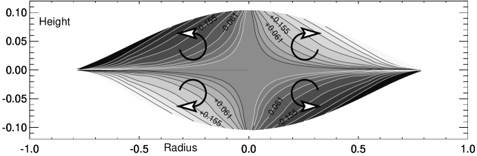
Figure 8: Section of the vorticity field for the caustic of Fig. (6). The local vorticity is antisymmetric with respect to the centre of the caustic. In this $X-Z$ section, it points along the Y-axis, and is negative in the second and fourth quadrant, positive in the first and third.

3.3.3 Scaling laws

We now bring forward fits to describe the dependence of the integrated vorticity with the spectral index $n$ and $\lambda_{\rm max.}$ which will allow us to characterize the most significant caustics that contribute to the large–scales vorticity. We make explicit the dependence of those quantities with respect to the size of the perturbation $R_{L}$ and the cosmological parameter $\Omega$. Expressed in units of the expansion factor, the displacement, in the Zel’dovich approximation, is independent of $\Omega$. Therefore $a$ and $b$ are independent of $\Omega$, and are simply proportional to $R_{L}$. The total vorticity in each quadrant is on the other hand proportional to $H_{0}$ and $f(\Omega)$ (defined in Eq. (34)), given that it is proportional to the local velocity, and is clearly proportional to the volume of the perturbation. We thus have the following scalings,

$$d(R_{L})=R_{L}\ d_{0}\ (\lambda_{\rm max}-1)^{\alpha_{d}},\ \ e(R_{L})=R_{L}\ e_{0}\ (\lambda_{\rm max}-1)^{\alpha_{e}},\ \ \omega_{\rm quad}(R_{L},\Omega)=f(\Omega)\ R_{L}^{D}\ \omega_{0}\ (\lambda_{\rm max}-1)^{\alpha}\,H_{0},$$ (47)

where the parameters $\alpha$, $\alpha_{d}$, $\alpha_{e}$, $\omega_{0}$, $d_{0}$ and $e_{0}$ are given in Table (1) and  (2) for respectively the 2D and the 3D geometry. The accuracy of these fits is illustrated on Figs. (10)– (10). These functions yield estimates of the geometry and vorticity generated by these large-scale caustics. From these tables one can see that the average vorticity (in units of $H_{0}$) is roughly one within the caustic. The amount of vorticity which is generated in the caustics is thus found to be somewhat limited. It is also interesting to note that $\omega_{\rm quad.}$ presents no singular behaviour when the caustic appears at $\lambda_{\rm max}\approx 1$ (i.e. $\alpha>1$).

Figure 9: $\omega_{\rm quad.}$ for 2D caustics as a function of $\lambda_{\rm max}$ and its corresponding fit for a $n=-1.5$ (circles, solid line), $n=-1$ (squares, long dash line), and $n=-0.5$ (triangles, short dashed line) power spectrum.

Figure 10: $\omega_{\rm quad.}$ for 3D caustics as a function of $\lambda_{\rm max}$ and its corresponding fit for a $n=-2$ (circles, solid line), $n=-1.5$ (squares, long dash line), and $n=-1$ (triangles, short dashed line) power spectrum.

Table 1: Fitting parameters in Eq. (47) for the 2D caustics. The quality of those fits for $\omega_{0}$ and $\alpha$ are illustrated in Fig. (10).

$n$	$\omega_{0}$	$\alpha$	$d_{0}$	$\alpha_{d}$	$e_{0}$	$\alpha_{e}$
-1.5	3.94	1.95	0.8	1.3	2.7	0.6
-1	1.80	1.59	0.67	1.3	1.6	0.45
-0.5	1.63	1.43	0.75	1.3	1.3	0.32

Table 2: Fitting parameters in Eq. (47) for the 3D caustics. The quality of those fits are illustrated in Fig. (10).

$n$	$\omega_{0}$	$\alpha$	$d_{0}$	$\alpha_{d}$	$e_{0}$	$\alpha_{e}$
-2	0.67	1.76	0.57	1.31	1.61	0.49
-1.5	0.46	1.55	0.52	1.30	1.25	0.37
-1	0.49	1.37	0.53	1.30	1.13	0.30

4 The vorticity distribution at large scales

As argued previously, the calculation of the global shape of the vorticity distribution is beyond the scope of this paper. Indeed the low $\omega$ behaviour of the vorticity distribution is dominated by the small caustics that are not rare, and therefore not well described by the dynamical evolution of an isolated object. The aim of this section is to estimate the shape and position of the cutoff in the probability distribution function of the local smoothed vorticity. We will therefore estimate $P_{R_{s}}(>\omega_{s})$, the probability that in a circular or spherical cell of radius $R_{s}$ the mean vorticity exceeds $\omega_{s}$. This estimation requires

• identifying the caustics that contribute mostly for each case;

• estimating the contribution of each of those caustics.

In each case various approximations are used. In the main text we simply spell the major highlights of the derivation. A more detailed and explicit calculation of the vorticity distribution is presented in Appendix C.

4.1 Identification of the caustics

We assume in what follows that $\omega_{s}$ is large enough for the contribution to $P_{R_{s}}(>\omega_{s})$ to be dominated by large and rare caustics. This assumption is the corner stone of the calculation: only a small fraction of the caustics with specific characteristics at some critical time will contribute.

The identification of the caustics contributing most results of a trade off between the amount of vorticity a given caustic can generate and its relative rarity: the higher $\lambda_{\rm max}$, the greater the internal vorticity is, according to Eq. (47) and given that $\alpha$ is positive, but the rarer those caustics are (Equations  (11) and  (17)). Obviously $\lambda_{\rm max}$ should be larger than unity for any vorticity at all to be generated. The calculation is slightly complicated by the fact that the Eulerian size of the caustics also depends of the value of $\lambda_{\rm max}$. Let us assume here that the Eulerian size of the caustics is substantially smaller than the smoothing length, so that the entire integrated vorticity in a quadrant can contribute (in Appendix C, this assumption is shown to be self-consistent). This implies a scaling relation between the smoothing cell, $\omega_{s}$ and $\lambda_{\rm max}$,

$$\omega_{s}\ R_{s}^{D}\propto R_{L}^{D}\ (\lambda_{\rm max}-1)^{\alpha}.$$ (48)

For a given smoothing length and a given $\omega_{s}$, Eq. (48) yields a relation between the value of $\lambda_{\rm max}$ and the size of the caustic. The caustics which contribute most to the vorticity are then obtained by minimizing the ratio $\lambda_{\rm max}^{2}/\sigma^{2}(R_{L})$ which appears in the exponential cutoff of the distribution function of $\lambda_{\rm max}$ (Equations  (11) and  (17)). Given that $\sigma^{2}(R_{L})$ behaves like $R_{L}^{-(n+D)}$ this minimization yields for the extremum value of $\lambda_{\rm max}$,

$$\lambda_{\rm max}^{(0)}={2D\over 2D-\alpha(n+D)}.$$ (49)

Note that for the values of $\alpha$ we have found, $\lambda_{\rm max}^{(0)}$ is always finite and positive. This means that the filtered vorticity is indeed expected to be dominated by caustics which have evolved for a finite time. This provides an a posteriori justification of the assumptions leading to this calculation.

The value of $\lambda_{\rm max}$ found in Eq. (49) is a robust result of our calculations, although it cannot be excluded that this value could be affected by the failure of the Zel’dovich approximation after the first shell crossing.

4.2 Estimation of the caustic contribution to the vorticity PDF

In order to estimate the contribution of those caustics to $P_{R_{s}}(>\omega_{s})$ two other fundamental quantities have to be estimated:

• the number density of caustics;

• the volume for which each of them contributes to $P_{R_{s}}(>\omega_{s})$.

These quantities have been estimated for the specific caustics we have previously identified in Sect. 4 1.

4.2.1 The number density of caustics

Estimating the number density of caustics is, in general, a complicated problem. In the case of Gaussian fields the corresponding investigation was carried by Bardeen et al. (1986) for 3D fields, and by Bond & Efstathiou (1987) for 2D fields. The number of caustics is simply determined by the number of points at which the first derivatives of the local density vanishes. This defines accordingly the extrema of the local density field. The further requirements we have here on the second order derivatives of the potential ensures that such points are in fact maxima of density field. We refer here to Bardeen et al. (1986) for more details on how to carry the investigation. A critical step involves transforming the $\delta_{\rm Dirac}$ function in the value of the first derivatives into a $\delta_{\rm Dirac}$ function in the position, thus introducing the Jacobian of the second order derivatives of the density field. After some algebra we find:

$$n_{R_{L}}(\{\lambda_{i}\})\,{\rm d}^{D}\lambda_{i}=p\left(\left\{\lambda_{i}\over\sigma(R_{L})\right\}\right)\,{{\rm d}^{D}\lambda_{i}\over\sigma^{D}(R_{L})}{|{\rm Jac}_{2}(\{\lambda_{i}\})|\over(2\pi\sigma_{1}^{2})^{D/2}}\,,$$ (50)

where the probability $p$ is given either by Eq. (9) or  (15) in respectively 2D and 3D, ${\rm Jac}_{2}(\{\lambda_{i}\})$ is the Jacobian of the second order derivatives of the density field for given eigenvalues of the deformation matrix and $\sigma_{1}$ is the variance of the derivatives of the local density field,

$$\sigma_{1}^{2}(R_{L})=\int{\rm d}^{D}k\ P(k)\ {{\bf k}^{2}\over 2}\ W_{D}^{2}(R_{L}).$$ (51)

For a given geometry (i.e. given values of $a$ and $b$) ${\rm Jac}_{2}$ is proportional to $\lambda_{\rm max}^{3}$, and it scales as $R_{L}^{-2\,D}$ due to the derivatives involved in the expression of the matrix elements. It is therefore appropriate to re-express Eq. (50) as

$$n_{R_{L}}(\{\lambda_{i}\})\,{\rm d}^{D}\lambda_{i}=p\left(\left\{\lambda_{i}\over\sigma(R_{L})\right\}\right)\,{{\rm d}^{D}\lambda_{i}\over\sigma^{D}(R_{L})}{n_{0}(\{\lambda_{i}\})\over R_{L}^{D}}\,\left({\lambda_{\rm max}\over\sigma(R_{L})}\right)^{D}\quad{\rm where}\quad n_{0}(\{\lambda_{i}\})={|{\rm Jac}_{2}(\{\lambda_{i}\})|\over\lambda_{\rm max}^{D}\ (2\pi)^{D/2}}\ \left[{\sigma\over\sigma_{1}}\right]^{D}\,R_{L}^{D}.$$ (52)

Note that $n_{0}$, thanks to the prefactor $R_{L}^{D}$, is a dimensionless quantity in Eq. (52). A further simplification is provided by the fact that for large enough values of $\lambda_{\rm max}$, the distribution function $p(\{\lambda_{i}\})$, at fixed $\lambda_{\rm max}$, allows only a small range of possible values for the smaller eigenvalues. We therefore neglect the variations of ${\rm Jac}_{2}(\{\lambda_{i}\})$ with respect to those variables: it is viewed here as a function of $\lambda_{\rm max}$ only and calculated for fixed values of the a-symmetry parameters $a$ and $b$. The ratio $\sigma/\sigma_{1}$ depends only on the value of the power law index. Recall however (see Bardeen et al. 1986) that this ratio is not well-defined for top-hat window functions because of spurious divergences for some values of $n$. To avoid this problem, we used the Gaussian window function to compute this ratio. As a result, for fixed values of $a$ and $b$, $n_{0}$ is a dimensionless quantity that can be explicitly calculated in a straightforward manner. Relevant values of $n_{0}$ are given in tables in the Appendix C.

4.3 The contributing region

The region over which each caustic contributes is the surface (or volume in 3D) of space in the vicinity of a given caustic where, if one centers a cell in that location, the total vorticity induced by the caustic within the cell is above $\omega_{s}$.

In general the contributing surface or volume can be written,

$$V_{\rm caus.}(R_{L},R_{s},\{\lambda_{i}\},\omega_{s})=\int\Theta\left[\omega_{\bf c}\left({\bf c},R_{L},R_{s},\{\lambda_{i}\}\right)-\omega_{s}\right]\,{\rm d}^{D}c\,,$$ (53)

where $\Theta$ is the Heaviside step function, $\bf c$ stands for the vector pointing to the center of the sampling sphere, while $\omega_{\bf C}$ is the vorticity found in that sphere intersecting the caustic with characteristics $R_{s},\{\lambda_{i}\}$. In its full generality, $V_{\rm caus.}$ is a rather complex function of the scales $R_{L}$ and $R_{s}$, and the eigenvalues ${\lambda_{i}}$ through the shape of the caustics and of $\omega_{s}$. Yet, since the functional form of the rare event tail in the probability distribution function is basically fixed by the exponential in Eq. (11), the only required ingredient for computing $P_{R_{s}}(>\omega_{s})$ is the scaling behaviour of $V_{\rm caus.}$ at its takeoff – when reaching the critical time, $\lambda_{\rm max}^{(0)}$, at which a given caustic is large enough to start contributing. The detailed geometry of the caustic and its vorticity field accounts only for a correction in a multiplicative factor. Consequently we make approximations describing the distribution of the vorticity on the caustic in order to estimate the scaling properties of $V_{\rm caus.}$.

4.3.1 The 2D contributing surface

In two dimensions we make the radical assumption that the vorticity is entirely concentrated on four discrete points, which – consistently with the hypothesis of Sect. 3.3.2, have been taken to bear either the vorticity $+\omega_{\rm quad.}$ or $-\omega_{\rm quad.}$, depending on which quadrant is being considered. In practice the position of the points is chosen somewhat arbitrarily at a third of the depth and extension of the caustic. The corresponding area $V_{\rm caus.}$ is therefore identically null before a critical time corresponding to the chosen $\omega_{s}$ and $R_{s}$ and then takes a constant value which can be deduced geometrically from the area of the loci of the center of the sampling disks. In Fig. (12) we show the shape of this location on a particular example. Under this assumption, the function $V_{\rm caus.}$ takes the form,

$$V_{\rm caus.}=V_{0}(R_{L}/R_{s})\ \Theta(\lambda_{\rm max}-\lambda_{\rm max}^{(0)})\,R_{L}\,R_{s}\,,$$ (54)

where $V_{0}$ can be calculated for the values of interest of $R_{L}$ and $R_{s}$.

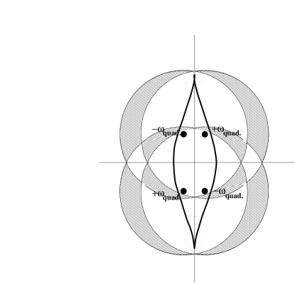
Figure 11: Sketch showing the adopted simplification for describing a 2D caustic. Vorticity is assumed to be localized on the black dots having either $+\omega_{\rm quad.}$ or $-\omega_{\rm quad.}$. The dashed area represents $V_{\rm caus.}$ for $\omega_{s}>|\omega_{\rm quad.}|$.

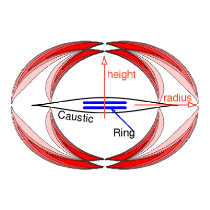
Figure 12: Sketch showing the adopted simplification for describing a 3D caustic. Vorticity is assumed to be localized on two rings (that appear as two horizontal black segments) having a lineic vorticity of either either $+3\,\omega_{\rm quad.}/e$ or $-3\,\omega_{\rm quad.}/e$. The shaded area represents ${\rm d}V_{\rm caus.}/{\rm d}\omega_{s}$.

4.3.2 The 3D contributing volume

In three dimensions, the vorticity will be assumed to be distributed uniformly along two rings which are taken to bear the linear vorticity $3\omega_{\rm quad.}/e$ – with respectively prograde and retrograde orientation. In practice these rings are also positioned at a third of the depth and extension of the caustic. The mean vorticity to be expected in a sampling sphere of radius $R_{s}$ is then given by algebraic summation over the segments corresponding to the intersection of that sphere with the two rings. Maps of the sampled vorticity as a function of the centers of the sphere are derived to compute $V_{\rm caus.}$ which according to Eq. (53) corresponds to the volume in space defined by these centers yielding a vorticity larger than $\omega_{s}$. Fig. (12) gives the shape of this location for a given caustic and sampling radius. The function $V_{\rm caus.}$ takes the form,

$$V_{\rm caus.}=V_{0}(R_{L}/R_{s})R_{L}R_{s}^{2}\ (\lambda_{\rm max}-\lambda_{\rm max}^{(0)})^{\gamma}\,,$$ (55)

where $V_{0}$ and $\gamma$ can be calculated for the values of interest of $R_{L}$ and $R_{s}$ at this critical values (see Appendix  D, where it is in particular demonstrated that when $R_{L}\ll R_{s}$, $V_{0}$ asymptotes to a fixed value and $\gamma=1/2$).

4.4 Estimation of $P_{R_{s}}(>\omega_{s})$

The tail of the probability distribution for the vorticity is now estimated while integrating over all the caustics that might contribute, and assuming that, for a fixed caustic, the probability distribution is given by the number density of caustics times the volume associated with each caustic. There is however a further difficulty. The distribution of caustics $n_{R_{L}}$ is well defined for a fixed value of $R_{L}$ only, but there are actually caustics of all sizes. To circumvent this difficulty we simply choose $R_{L}$ so that the result we obtain is maximal, i.e.,

$$P_{R_{s}}(>\omega_{s})\simeq\max_{R_{L}}\left[\int{\rm d}^{D}\lambda_{i}\ n_{R_{L}}(\{\lambda_{i}\})\ V_{\rm caus.}(R_{L},R_{s},\{\lambda_{i}\},\omega_{s})\right]\,.$$ (56)

Furthermore, it is fair to neglect the dependence of $n_{0}({\lambda_{i}})$ and $V_{\rm caus}$ on the initial asymmetry because the overall factor $p({\lambda_{i})}$ peaks in a narrow range of relevant values for the smaller eigenvalue(s). It is then possible to integrate over those variables introducing the probability distribution of $\lambda_{\rm max}$ in the expression of $P_{R_{s}}(>\omega_{s})$,

$$P_{R_{s}}(>\omega_{s})\simeq\max_{R_{L}}\left[\int{{\rm d}\lambda_{\rm max}}\ p_{\rm max}\left({\lambda_{\rm max}}\right)\,{n_{0}(\lambda_{\rm max})\over R_{L}^{D}}\,\left({\lambda_{\rm max}\over\sigma(R_{L})}\right)^{D}V_{\rm caus.}(R_{L},R_{s},\lambda_{\rm max},\omega_{s})\right]\,.$$ (57)

We show in Appendix C that the maximum of Eq. (56) is indeed given by caustics of size of the order of $R_{s}$ at most. A detailed account of how to perform the sum in Eq. (56) is also given there for the two geometries. Repeated use of the rare event approximation together with the geometrical assumptions on the vorticity distribution sketched in Sect. 4.3.1 and Sect. 4.3.2 yields eventually an explicit expression for the tail of the probability distribution for the vorticity as a function of $\omega_{s}$ and $R_{s}$.

4.4.1 The two dimensional vorticity distribution

In two dimensions, the vorticity distribution is shown to obey (Eq. (101))

$$P_{R_{s}}(>\omega_{s})\simeq 0.56\,n_{0}\,V_{0}\,\left({\lambda_{\rm max}^{(0)}\over\sigma(R_{s})}\right)^{2}\,f_{s}^{n+1}\,\omega_{s}^{(n+1)/2}\,\exp\left[-{4\over 3}\,\left({\lambda_{\rm max}^{(0)}\over\sigma(R_{s})}\right)^{2}\,f_{s}^{n+2}\,\omega_{s}^{(n+2)/2}\right].$$ (58)

In the rare event régime, the quantity that dominates Eq. (58) arises from the exponential cutoff. For $n=-1$ we find for instance that

$$\log\left[P_{R_{s}}(>\omega_{s})\right]\simeq 3.5\,{\omega_{s}^{1/2}\over\sigma^{2}(R_{s})}.$$ (59)

The r.h.s. of Eq. (59) is roughly $0.5$ when $\omega_{s}\approx 10^{-3},\ \sigma(R_{s})\approx 0.5$ or $\omega_{s}\approx 0.1,\ \sigma(R_{s})\approx 1.5$, hence defining a threshold corresponding to a one sigma damping for $P_{R_{s}}(>\omega_{s})$. Equation  (58) is illustrated on Fig. (14).

4.4.2 The three dimensional vorticity distribution

Similarly, the probability distribution is shown in the Appendix C (Eq. (111)) to obey in 3D:

$$P_{R_{s}}(>\omega_{s})=0.48\,n_{0}\,V_{0}\,\left({\lambda_{\rm max}^{(0)}\over\sigma(R_{s})}\right)^{7/2}\,f_{s}^{(13+7n)\over 4}\,\omega_{s}^{(13+7n)\over 12}\,\exp\left[-{5\over 2}\,\left({\lambda_{\rm max}^{(0)}\over\sigma(R_{s})}\right)^{2}\,f_{s}^{n+3}\,\omega_{s}^{(n+3)/3}\right],$$ (60)

For $n=-1.5$, Eq. (60) gives for $\log\left[P_{R_{s}}(>\omega_{s})\right]$

$$\log\left[P_{R_{s}}(>\omega_{s})\right]\simeq 20.\,{\omega_{s}^{1/3}\over\sigma^{2}(R_{s})}.$$ (61)

yielding again at a one sigma level the range of relevant values for $\omega_{s}$ and $\sigma(R_{s})$: $\omega_{s}\approx 5\,10^{-5},\ \sigma(R_{s})\approx 0.5$ or $\omega_{s}\approx 0.1,\ \sigma(R_{s})\approx 3.5$. In both cases the caustics start to generate significant vorticity only at rather small scales. Equation  (60) is also illustrated on Fig. (14). From this figure it is clear that the amount of vorticity that we derived is below what has been measured in $N$-body simulations (open and filled circles). Numerical measurements of this quantity are sparse, so we compared our estimations to measurements carried out by Bernardeau & Van de Weygaert (1996) in an adaptive P³M simulation with CDM initial conditions (see Couchman 1991 for a description of these simulations). The typical amount of vorticity at the $10$ to $15$ $h^{-1}$Mpc scale for which the rms of the density is below $0.5$ was found to be about $0.2$ (in units of $H_{0}$). This is well above the values we have estimated in this paper. Though it is quite possible that these numerical measurements are spoiled by noise, we do not expect that it could account for all the discrepancy between the measured and the predicted vorticities (as suggested by the relative the scatter between the two methods suggested in Bernardeau & Van de Weygaert, 1996).

There are various possible explanations for such discrepancies. It could of course arise from the fact that the vorticity at large-scales does not spring from the rare and large caustics but from small scale multi-steaming events that cascade towards the larger scales. Such a scenario cannot be excluded but is difficult to investigate by means of analytic calculations. It is also possible that the $N$-body simulations do not address properly the physics of the large scales multi-streaming. In particular the two-body interactions should in principle be negligible, a property which seems to be hardly satisfied in current $N$-body simulations. This shortcoming has been raised by Suisalu & Saar (1995), Steinmetz & White (1997) and more specifically by Splinter et al. (1998), where they examine the outcome of the planar singularity in phase space. They have found in particular that in classical algorithms the particle’s velocity dispersions are incorrectly large in all directions. These could turn out to be a major unphysical source of vorticity (since the Lagrangian time derivative of the vorticity scales like the curl of the divergence of the velocity anisotropies). Specific numerical experiments, that follow for instance the initial density profiles given in this paper, should be carried to address this problem more carefully.

Figure 13: $P_{R_{s}}(>\omega_{s})$ in two dimensions for scales characterized by a $\sigma(R_{s})$ of $0.5$ (thick lines) and $1$ (thin lines) and for a $n=-1.5$ (solid line), $n=-1$ (long dash line), and $n=-0.5$ (short dashed line) power spectrum.

Figure 14: $P_{R_{s}}(>\omega_{s})$ in three dimensions for scales characterized by a $\sigma(R_{s})$ of $0.5$ (thick lines) and $1$ (thin lines) and for a $n=-2$ (solid line), $n=-1.5$ (long dash line), and $n=-1$ (short dashed line) power spectrum. The filled and open circles correspond respectively to the measured integrated PDF in a CDM simulation at $15h^{-1}$Mpc scale with the “Delaunay” or “Voronoi” methods (see Bernardeau & Van de Weygaert 1996).

5 Discussion and Conclusions

We have estimated, within the framework of the gravitational instability scenario, the amount of vorticity generated after the first shell crossings in large-scales caustics. The calculations relied on the Zel’dovich approximation which yields estimates of the characteristics of the largest caustics and allows explicit calculation of their vorticity content. This analysis corresponds to one of the first attempts to investigate the properties of cosmological density perturbations beyond first shell-crossing. The previous investigations (Fillmore & Goldreich 1984, Bertschinger 1985) were carried out for spherically symmetric systems only, and obviously do not address the physics of vorticity generation. The only other means of investigation for this régime is numerical $N$-body simulations.

We found that large scales caustics can provide only an extremely low contribution to the vorticity at scales of $10$ to $15h^{-1}{\rm Mpc}$. This contribution could be significant only at relatively small scales, when the variance reaches values of a few units. This effect is even more important in three dimensions, the difference arising mainly from the coefficient in the exponential cut-off. It is therefore unlikely that these caustics can have produced a significant effect on the velocity at large scales. In view of these results, it is amply justified to assume that the velocity remains potential down to very small scales, i.e. typically the cluster scale at which it is then more natural to expect the multi-streaming régime (not only three-flow régime) to play an important role.

This result provides a complementary view to the picture developed by Doroshkevich (1970) describing the emergence of galaxy angular momentum from small-scale torque interactions between protogalaxies (a prediction subsequently checked by White (1984), and examined in more detail by Catelan & Theuns, (1996 and 1997)). We rather explore here the large scale coherence of the vorticity field that may emerge in a hierarchical scenario from scale much larger than the galactic size. The effects we are exploring here does not originate from the two-body interaction of haloes as in the picture developed by Doroshkevich, but from the possible existence of large scale coherent vorticity field. The conclusion of our work is however that the efficiency with which the large-scale structure caustics generate vorticity is rather low. Therefore these results do not really challenge the fact that the small scales interactions should indeed be the dominant contribution to the actual galactic angular momenta.

As a consequence, we do not expect either a significant correlation of the angular momenta at large scale. In particular the vorticity field generated in caustics does not seem to be able to induce a significant large scale correlation of the galactic shapes which would have been desastruous for weak lensing measurements.

Let us reframe this calculation in the context of perturbation theory which has triggered some interest in the last few years as a tool to investigate the quasi-linear growth of structures. One key assumption in these techniques is that the velocity field is assumed to form a single potential flow. The detailed description of the properties of the first singularities is by essence not accessible to this theory: such singularities cannot be “seen” through Taylor expansions of the initial fields. In this context it was unclear whether the back reaction of the small scales multi-streaming régime on the larger scales (which were thought to be adequately described by perturbation theory) could affect the results on those scales. Such effects are partially explored here where we find that the impact of the first multistreaming regions is rather low on larger scales. Our results therefore support the idea that the large scales velocity field can be accurately described by potential flows and support our views on the validity domain of perturbation theory calculations.

In the course of this derivation we have made various assumptions. We followed in essence the approach pioneered by Press & Schechter (1974) for the mass distribution of virialized objects by trying to identify in the initial density field the density fluctuations that contribute mostly to the large-scales vorticity. The calculations have been designed to be as accurate as possible in the rare event limit, an approximation which turned out to be crucial at various stages of the argument.

• The above estimation relies heavily on the assumption that the caustics only contribute to large-scale vorticity independently of each other. In other words it is assumed that the caustics do not overlap. Moreover the dynamical evolution of one caustic is taken to be well-described by the evolution of the caustic having the mean profile. This can be approximately true only in the rare event limit since otherwise it is likely that the substructures and its environment will change the dynamical evolution of the caustics. Although it is clear that, in the régime we investigated, the caustics are rare enough not to overlap, the effects of substructure are more difficult to investigate. In particular we have outlined some local features (3.3.1) of the vorticity maps that we think are unlikely to survive the existence of substructures.

• The typical caustics are characterized in this rare event limit. For instance the values of $a$ and $b$ were found to be all the more peaked to given values as the corresponding events are rare. We have then estimated the vorticity such caustics generate while assuming that slightly different geometries are unlikely to produce very different results. This assumption is somewhat suspicious, since it might turn out that slightly different geometries could produce more vorticities, and thus change the exact position of the cut-off. We do not expect however that the conclusions we have reached could be changed drastically in this manner.

• The contributions of each caustics to $P_{R_{s}}(>\omega_{s})$ have also been calculated in the rare event limit. This is in practice a very useful approximation on large scales since it is then natural to expect the entire distribution to be dominated by a unique value of $\lambda_{\rm max}$.

• We have finally deliberately simplified the spatial distribution of the vorticity within the caustics. Since in the rare event limit it is natural to expect that the Lagrangian scales of the caustics are much smaller than the smoothing scale this detailed arrangement should be of little relevance. It certainly should not affect the scaling laws as only the value of the overall factor $V_{0}$ will change, and this has little bearing on our conclusions.

On top of the rare event limit approximation, we have also made a dramatic simplification by using the Zel’dovich approximation throughout. This is certainly a secure assumption before the first shell-crossing since the geometries that we have investigated were rather sheet-like structures (and the Zel’dovich approximation is exact in 1D dynamics). After the first shell-crossing however, the back reaction of the large over-densities that are created could possibly affect the velocity field. However we do not expect that this effect should be very large so long as $\lambda_{\rm max}$ is moderately small (up to about 1.5), since before then the initial inertial movement should dominate. Later on, matter is expected to bounce back to the center of the caustics. Whether the vorticity content is then amplified or reduced remains an open question.

CP wishes to thank J.F. Sygnet, D. Pogosyan, S. Colombi and J.R. Bond for useful conversations. Funding from the Swiss NF is gratefully acknowledged.

Appendix A Average profile of an a-spherical constrained random field

A.1 General Formula

Let us evaluate here the average profile of an a-spherical constrained random field in both 2 and 3D. Similar calculations as those presented in this Appendix have been investigated by Bardeen et al. (1986) for the 3D field and by Bond & Efstathiou (1987) for 2D fields. But, here, instead of the second order derivative of the density field, we consider instead the deformation tensor corresponding to second order derivatives of the potential. We also investigate the global properties that such constraints induce on the density field.

Consider a random density field, in either 2D or 3D, having fluctuations following a Gaussian statistics. It is then entirely determined, in a statistical sense, by the shape of its power spectrum, $P(k)$. Recall that $P(k)$ is defined from the Fourier transform of the density field,

$$\delta({\bf k})=\int{\rm d}^{3}{\bf x}\exp({\rm i}{\bf k}.{\bf x})\ \delta({\bf x})\,,\ \ {\rm with}\ \ \big{<}\delta({\bf k})\,\delta({\bf k}^{\prime})\big{>}=\delta_{\rm Dirac}({\bf k}+{\bf k}^{\prime})\,P(k),$$ (62)

where the brackets $\big{<}.\big{>}$ stands for the ensemble average of the random variables. Let us calculate the expectation value of $\delta({\bf k})$ when a local constraint has been set in order to create an a-spherical perturbation. To set such a constraint, we have chosen to consider the deformation tensor of the density field smoothed at a given scale $R_{L}$. This tensor reads,

$$\phi_{i,j}=\int{\rm d}^{3}{\bf k}\ \delta({\bf k})\ W_{D}(k\,R_{L})\ {{\bf k}_{i}{\bf k}_{j}\over k^{2}}.$$ (63)

Note that the local smoothed density is given by the trace of this tensor. The chosen window function $W_{D}$ in Fourier space corresponds to a top-hat filter in real space and it reads,

$$W_{2}(k)=2\ {J_{1}(k)\over k^{1/2}}\quad{\rm in\ }\ \ 2D,\ \ W_{3}(k)=3\sqrt{\pi/2}\ {J_{3/2}(k)\over k^{3/2}}\ \ {\rm in\ }\ \ 3D,$$ (64)

where $J_{\nu}$ are the Bessel functions of index $\nu$. The matrix $\phi_{i,j}$ is now set to be equal to a given constraint. It is obviously possible to choose the axis so that this constraint is a diagonal matrix with eigenvalues $(\lambda_{i}),i=1,D$. The elements of the matrix $\phi_{i,j}$ and $\delta({\bf k})$ form a Gaussian random vector,

$$\begin{array}[]{cl}V_{c}=\left(\delta({\bf k}),\phi_{1,1},\dots,\phi_{D,D},\phi_{1,2},\dots,\phi_{1,D},\right.\left.\phi_{2,2},\dots,\phi_{D,D-1}\right),\end{array}$$ (65)

and the desired expectation value of $\delta({\bf k})$ is directly related to the cross-correlation matrix of the components of this vector. Consider the matrix $C_{a,b}$ with $a=0,\cdots D(D+1)/2$ and $b=0,\cdots D(D+1)/2$, so that

$$C_{0,0} = \big{<}\delta({\bf k})\,\delta({\bf k})\big{>}=P(k)\,,$$ (66)

$$C_{a,0} = \big{<}\delta({\bf k})\,\phi_{i,j}\big{>}=P(k)\,W_{D}(k\,R_{L})\,{{\bf k}_{i}{\bf k}_{j}\over k^{2}}\,,$$ (67)

$$C_{a,b} = \big{<}\phi_{i,j}\,\phi_{i^{\prime},j^{\prime}}\big{>}=\int{\rm d}^{3}{\bf k}\ P(k)\,W_{D}^{2}(k\,R_{L}){{\bf k}_{i}{\bf k}_{j}{\bf k}_{i^{\prime}}{\bf k}_{j^{\prime}}\over k^{4}}\,,$$ (68)

where the indices ${i,j}$ (respectively ${i^{\prime},j^{\prime}}$) for the matrix elements $\phi_{ij}$ corresponds to the $(a+1)^{\rm th}$ (respectively $(b+1)^{\rm th}$) component of $V_{c}$. For a given spectrum these quantities are easily calculated and are given in the following subsections for power law spectrum in resp. 2 and 3 dimensions. The distribution function of the components of the vector $V_{c}$ then reads in terms of Eq. (68),

$$p(V_{c})\,{\rm d}V_{c}=\exp\left[-{1\over 2}\sum_{a,b}\,\left(C^{-1}\right)_{a,b}\,Vc_{a}\,Vc_{b}\right]\,{{\rm d}V_{c}\over[2\pi{\rm Det}(C)]^{1/2+D(D+1)/4}}.$$ (69)

The expectation value of $\delta({\bf k})$ is given by the ratio

$$\delta^{\rm expec.}({\bf k})={\int{\rm d}\delta({\bf k})\ \delta({\bf k})\ p(Vc)\over\int{\rm d}\delta({\bf k})\ p(Vc)}\,,$$ (70)

A straightforward calculation shows that this quantity is given by

$$\delta^{\rm expec.}({\bf k})=\sum_{i=1}^{D}-{\left(C^{-1}\right)_{0,i}\over\left(C^{-1}\right)_{0,0}}\ \lambda_{i}\,.$$ (71)

Note that the further constraint that the first derivative of the density field should be zero (so that the point $x_{0}$ is actually located on a maximum of the density field) would not change the resulting expression of $\delta^{\rm expec.}({\bf k})$ since the cross correlation of the first order derivatives with any other involved quantities identically vanish.

A.2 The 2D profile

In 2 dimensions we have

$$C_{a,b}=\left(\begin{array}[]{cccc}C_{0,0}&C_{0,1}&C_{0,2}&C_{0,3}\\ C_{0,1}&3\sigma_{0}^{2}/8&\sigma_{0}^{2}/8&0\\ C_{0,2}&\sigma_{0}^{2}/8&3\sigma_{0}^{2}/8&0\\ C_{0,2}&0&0&\sigma_{0}^{2}/8\end{array}\right)\,,$$ (72)

with the variance of the smoothed density field, $\sigma_{0}$, given by

$$\sigma_{0}^{2}=\int{\rm d}^{3}{\bf k}\ P(k)\ W^{2}_{D}(k\,R_{L}).$$ (73)

The required elements of the inverse of this matrix are given by

$$\left(C^{-1}\right)_{0,0} = {1\over 64}\sigma_{0}^{6}/{\rm Det}(C)\,,$$ (74)

$$\left(C^{-1}\right)_{0,1} = -\left|\begin{array}[]{ccc}C_{0,1}&C_{0,2}&C_{0,3}\\ \sigma_{0}^{2}/8&3\sigma_{0}^{2}/8&0\\ 0&0&\sigma_{0}^{2}/8\end{array}\right|\ {1\over 64\ {\rm Det}(C)}={\left(C_{0,2}-3\,C_{0,1}\right)\sigma_{0}^{4}\over 64\ {\rm Det}(C)}\,,$$ (78)

$$\left(C^{-1}\right)_{0,2} = \left|\begin{array}[]{ccc}C_{0,1}&C_{0,2}&C_{0,3}\\ \sigma_{0}^{2}/8&\sigma_{0}^{2}/8&0\\ 0&0&\sigma_{0}^{2}/8\end{array}\right|\ {1\over 64\ {\rm Det}(C)}={\left(C_{0,1}-3\,C_{0,2}\right)\sigma_{0}^{4}\over 64\ {\rm Det}(C)}\,.$$ (82)

As a result, Eq. (71) becomes here

$$\delta^{\rm expec.}({\bf k})={P(k)\,W_{2}(k\,R_{L})\over\sigma_{0}^{2}}\left(\lambda_{1}+\lambda_{2}+2\cos(2\theta)[\lambda_{1}-\lambda_{2}]\right)\,,$$ (83)

where the angle $\theta$ were chosen so that

$$k_{1}/k=\cos(\theta)\,,\quad k_{2}/k=\sin(\theta).$$

$\theta$ the angle between a given vector and the eigenvector associated to the first eigenvalue.

A.3 The 3D profile

In 3 dimensions the matrix $C$ reads,

$$C=\left(\begin{array}[]{ccc}C_{0,0}&\dots&C_{0,6}\\ \vdots&D&\\ C_{0,6}&&\end{array}\right)\,,\quad{\rm with}\quad D={\sigma_{0}^{2}\over 15}\left(\begin{array}[]{cccccc}3&1&1&&&\\ 1&3&1&&0&\\ 1&1&3&&&\\ &&&1&0&0\\ &0&&0&1&0\\ &&&0&0&1\\ \end{array}\right).$$ (84)

From this expression of the matrix of the cross correlations it is quite straightforward to re-express Eq. (71) as

$$\delta^{\rm expec.}({\bf k})={3P(k)\,W_{3}(k\,R_{L})\over 2}\left(\lambda_{1}[{\bf k}_{2}^{2}+{\bf k}_{3}^{2}-4{\bf k}_{1}^{2}]+\right.\left.\lambda_{2}[{\bf k}_{1}^{2}+{\bf k}_{3}^{2}-4{\bf k}_{2}^{2}]+\lambda_{3}[{\bf k}_{1}^{2}+{\bf k}_{2}^{2}-4{\bf k}_{3}^{2}]\right).$$ (85)

When the coordinates of the wave vector are expressed in terms of the angles $\theta_{k}$ and $\phi_{k}$, defined by

$$k_{1}=k\,\sin(\theta_{k})\ \cos(\phi_{k})\quad k_{2}=k\,\sin(\theta_{k})\ \sin(\phi_{k})\quad{\rm and}\quad k_{3}=k\,\cos(\theta_{k})\,.$$

Eq. (85) becomes

$$\delta^{\rm expec.}({\bf k})={3\,P(k)\,W_{3}(k\,R_{L})\over 8\,\sigma_{0}^{2}}\,(\lambda_{1}+\lambda_{2}+6\lambda_{3})\left(1+a\,\cos(2\theta_{k})+b\,\cos(2\phi_{k})[1+\cos(2\theta_{k})]\right)\,,$$ (86)

where $a$ and $b$ are specific combinations of the eigenvalues,

$$a=5\,{2\lambda_{3}-\lambda_{1}-\lambda_{2}\over\lambda_{1}+\lambda_{2}+6\lambda_{3}}\,,\quad{\rm and}\quad b=5\,{\lambda_{1}-\lambda_{2}\over\lambda_{1}+\lambda_{2}+6\lambda_{3}}.$$ (87)

Appendix B The DF of the eigenvalues of the local deformation tensor

The derivation of the distribution function of the eigenvalues of the local deformation tensor was carried in 3D by Doroshkevich (1970). We extend here the calculation to the 2D case (for which the calculations are straightforward). Starting with equation  (72) – the cross-correlations between the elements of the deformation tensors, one can easily get the expression of the joint distribution function of the deformation tensor elements,

$$p(\phi_{1,1},\phi_{1,2},\phi_{2,2})\ {\rm d}\phi_{1,1}\ {\rm d}\phi_{1,2}\ {\rm d}\phi_{2,2}={8\over(2\pi)^{3/2}}\ {{\rm d}\phi_{1,1}\ {\rm d}\phi_{1,2}\ {\rm d}\phi_{2,2}\over\sigma_{0}^{3}}\ \exp\left[-{1\over 2}\left(3\phi_{1,1}^{2}+8\phi_{1,2}^{2}+3\phi_{2,2}^{2}-2\phi_{1,2}\phi_{2,2}\right)\right]$$ (88)

The change of variables,

$$\lambda_{+}={\phi_{1,1}+\phi_{2,2}\over 2}+{\sqrt{\Delta}\over 2}\,,\quad\lambda_{-}={\phi_{1,1}+\phi_{2,2}\over 2}-{\sqrt{\Delta}\over 2}\,,\quad{\rm with}\quad\Delta=(\phi_{1,1}-\phi_{2,2})^{2}+4\phi_{1,2}^{2},$$ (89)

allows us to introduce the eigenvalues of the matrix. The Jacobian $J$ of this transformation is given by

$$\begin{array}[]{cl}J^{-1}=\left|\begin{array}[]{ccc}{1\over 2}+{\phi_{1,1}-\phi_{2,2}\over 2\sqrt{\Delta}}&\sim&{1\over 2}-{\phi_{1,1}-\phi_{2,2}\over 2\sqrt{\Delta}}\\ \\ {1\over 2}-{\phi_{1,1}-\phi_{2,2}\over 2\sqrt{\Delta}}&\sim&{1\over 2}-{\phi_{1,1}+\phi_{2,2}\over 2\sqrt{\Delta}}\\ \\ 0&1&0\end{array}\right|=\sqrt{1-4\,\phi_{1,2}/\Delta}\end{array}\,.$$ (90)

As a result we have

$$p(\lambda_{+},\lambda_{-},\phi_{1,2})\ {\rm d}\lambda_{+}\ {\rm d}\lambda_{-}\ {\rm d}\phi_{1,2}={8{\rm d}\lambda_{+}\ {\rm d}\lambda_{-}\ {\rm d}\phi_{1,2}\over(2\pi)^{3/2}\sigma_{0}^{3}}\ {1\over\sqrt{1-4\,\phi_{1,2}/\Delta}}\ \exp\left[-{1\over\sigma_{0}^{2}}\big{(}{3\over 2}J_{1}^{2}-4J_{2}\big{)}\right]\,,$$

with

$$J_{1}=\lambda_{+}+\lambda_{-}\ ,,\quad{\rm and}\quad J_{2}=\lambda_{+}\ \lambda_{-}.$$ (91)

The integration over $\phi_{1,2}$ yields

$$\begin{array}[]{l}p(\lambda_{+},\lambda_{-})\ {\rm d}\lambda_{+}\ {\rm d}\lambda_{-}=\sqrt{2\over\pi}\ {{\rm d}\lambda_{+}\ {\rm d}\lambda_{-}\over\sigma_{0}^{3}}|\lambda_{+}-\lambda_{-}|\ \exp\left[-{1\over\sigma_{0}^{2}}\big{(}{3\over 2}J_{1}^{2}-4J_{2}\big{)}\right].\end{array}$$ (92)

Note that if $\lambda_{+}$ is a priori assumed to be greater than $\lambda_{-}$ the distribution should be multiplied by 2.

Appendix C Estimation of $P_{R_{s}}(>\omega_{s})$

In this Appendix we estimate the probability $P_{R_{s}}(>\omega_{s})$ that a sphere of radius $R_{s}$ contains an integrated vorticity larger than $\omega_{s}$. In order to account for caustics of all sizes we argued in the main text that $P_{R_{s}}(>\omega_{s})$ was well approximated by

$$P_{R_{s}}(>\omega_{s})\simeq\max_{R_{L}}\left[\int{\rm d}^{D}\lambda_{i}\ n_{R_{L}}(\lambda_{i})\ V_{\rm caus.}(R_{L},R_{s},\{\lambda_{i}\},\omega_{s})\right]\,.$$ (93)

We will now show that the maximum is indeed given by caustics of size of the order of $R_{s}$ and approximate this integral in 2 and 3D. To simplify further Eq. (93), note first that the distribution function of the eigenvalues is peaked in a given geometry (i.e. $a=1$, and $b\simeq 0$ in 3D) for rare caustics (large values of $\lambda_{\rm max}$). Therefore the integral in Eq. (93) will be dominated by caustics of this geometry and the factor $V_{\rm caus.}$ can be taken at this point while carrying the integration over the other two eigenvalues. As a result we have

$$P_{R_{s}}(>\omega_{s})\simeq\max_{R_{L}}\left[\int_{1}^{\infty}{\rm d}\lambda_{\rm max}\ p_{\rm max}(\lambda_{\rm max})\ \left({\lambda_{\rm max}\over\sigma(R_{L})}\right)^{D}\,{n_{0}(\lambda_{\rm max})\ V_{\rm caus.}(R_{L},R_{s},\lambda_{\rm max},\omega_{s})\over R_{L}^{D}}\right].$$ (94)

This integral runs from 1 to infinity since the caustics exist only when $\lambda_{\rm max}$ is greater than 1. The evaluation of Eq. (94) requires insights into the function $V_{\rm caus.}$. Although there are no real qualitative changes between the the 2D and 3D cases, we now proceed with the computation of Eq. (94) by distinguishing the two geometries for the sake of clarity.

C.1 The 2D statistics

Recall that the integral Eq. (93) will be dominated by the rare even tail, and thus by the lowest value of $\lambda_{\rm max}$ that contributes to the integral. In other words, when considering a given caustic characterized by its Lagrangian scale $R_{L}$, one should wait long enough so that it has grown sufficiently in order to contribute after sampling a vorticity larger than $\omega_{s}$. For each $R_{L}$ therefore corresponds $\lambda_{\rm max}^{(0)}(R_{L})$, the lowest value of $\lambda_{\rm max}$ for which $V_{\rm caus.}$ is non zero:

$$P_{R_{s}}(>\omega_{s})\simeq\max_{R_{L}}\left[\int_{\lambda_{\rm max}^{(0)}}^{\infty}{\rm d}\lambda_{\rm max}\ p_{\rm max}(\lambda_{\rm max})\ \left({\lambda_{\rm max}\over\sigma(R_{L})}\right)^{2}\,{n_{0}(\lambda_{\rm max})\,V_{\rm caus.}(R_{L},R_{s},\lambda_{\rm max},\omega_{s})\over R_{L}^{2}}\right].$$ (95)

The lower bound $\lambda_{\rm max}^{(0)}(R_{L})$ is reached as soon as $\omega_{\rm quad.}$ is larger than $\pi\ R_{s}^{2}\ \omega_{s}$: the largest possible value of the integrated vorticity in a cell of a given radius. It is therefore implicitly defined by

$${\omega_{s}={\omega_{\rm quad.}\over\pi\ R_{s}^{2}}\equiv\omega_{M}=f(\Omega)\ {R_{L}^{2}\over\pi R_{s}^{2}}\omega_{0}\ (\lambda_{\rm max}^{(0)}(\omega_{s},R_{L})-1)^{\alpha}}\,.$$ (96)

Assuming that $V_{\rm caus.}$ does not contain any exponential cutoff, and assuming that $\lambda_{\rm max}$ is in the rare event tail, Eq. (94) can be approximatively re-expressed as

$$P_{R_{s}}(>\omega_{s})\simeq\max_{R_{L}}\left[0.56\ \left({\lambda_{\rm max}^{(0)}\over\sigma(R_{L})}\right)^{2}\ \exp\left[-{4\over 3}\left({\lambda_{\rm max}^{(0)}\over\sigma(R_{L})}\right)^{2}\right]{n_{0}\,V_{\rm caus.}(R_{s},R_{L},\lambda_{\rm max}^{(0)},\omega_{s})\over R_{L}^{2}}\right],$$ (97)

when using Eq. (11) for the distribution function of $\lambda_{\rm max}$, integrating by part and dropping the residual integral for large enough ${\lambda_{\rm max}^{(0)}/\sigma(R_{L})}$ (see Appendix E for details). This maximum with respect to $R_{L}$ is then approximated by the minimum of the argument of the exponential, ${\lambda_{\rm max}^{{(0)}}(R_{L})/\sigma(R_{L})}$, where the minimum in the facto taken with respect to $\lambda_{\rm max}^{(0)}$ since $\sigma(R_{L})$ can be thought of a function of $\lambda_{\rm max}^{{(0)}}$ via Eqs. (22) and  (96). This minimum can de facto be expressed independently of $R_{s}$. It reads

$$\lambda_{\rm max}^{(0)}=\displaystyle{4\over 4-\alpha(n+2)}.$$ (98)

Once $\lambda_{\rm max}^{(0)}$ is fixed the geometry of the caustic which will contribute most to $P_{R_{s}}(>\omega_{s})$ is entirely specified. The condition for the existence of a minimum defining $\lambda_{\rm max}^{(0)}$ is that $\alpha(n+2)<4$, and it is satisfied for all considered cases (see Table (1)). This implies that we are investigating a régime where the integral Eq. (94) is not dominated by arbitrarily rare caustics – which would have been catastrophic given the assumptions (note that when $n$ is too large $\lambda_{\rm max}^{(0)}$ tend to be quite large thus challenging the validity of quantitative results based upon the Zel’dovich approximation). The resulting value of $R_{L}$ is

$$R_{L}=\displaystyle{R_{s}\ \sqrt{{\pi\omega_{s}\over\omega_{0}\,f(\Omega)}\,}\,\left({4-\alpha\,(n+2)\over\alpha\,(n+2)}\right)^{\alpha/2}}=f_{s}\ R_{s}\ \left({\omega_{s}\over f(\Omega)}\right)^{1/2}.$$ (99)

The scale factor $f_{s}$ is given in Table (3) for an Einstein-de Sitter universe ($f(\Omega)=1$) and different values of $n$. Completing the calculation of $P_{R_{s}}(>\omega_{s})$ involves relating the shape and size of the caustic for the adopted value of $\lambda_{\rm max}^{(0)}$. These values are derived from the fits (Eq. (47)) and are given in Table (3). Fig. (12) gives $V_{\rm caus.}$, in units of the square of $R_{L}$, as a function of the smoothing radius $R_{s}$. From Fig. (12) it is easy to see that

$$V_{\rm caus.}\simeq V_{0}\ R_{s}\,R_{L}\,,$$ (100)

for any values and $n$; the corresponding values of $V_{0}$ are given in Table 3. Putting Eq. (100) into Eq. (95), using Eqs. (98),  (99) yields for the sought distribution

$$P_{R_{s}}(>\omega_{s})\simeq 0.56\,n_{0}\,V_{0}\,\left({\lambda_{\rm max}^{(0)}\over\sigma(R_{s})}\right)^{2}\,f_{s}^{n+1}\,\omega_{s}^{(n+1)/2}\,\exp\left[-{4\over 3}\,\left({\lambda_{\rm max}^{(0)}\over\sigma(R_{s})}\right)^{2}\,f_{s}^{n+2}\,\omega_{s}^{(n+2)/2}\right],$$ (101)

Note that the power of $\omega_{s}$ in the exponential is rather weak. The cut-off is nonetheless strong in the régime of interest because of the leading coefficient. Equation  (101) is illustrated on Fig. (14) and discussed in the main text.

Table 3: Parameters of interest for the 2D caustics: the power index, $n$, the critical time $\lambda_{\rm max}^{(0)}$, the radial extension $e^{(0)}$, depth $d^{(0)}$ in units of $R_{L}$,scale factor $f_{s}^{(0)}$ as well as the values of $n_{0}$ and $V_{0}$ for the critical caustics.

$n$	$\lambda_{\rm max}^{(0)}$	$d^{(0)}$	$e^{(0)}$	$f_{s}$	$n_{0}$	$V_{0}$
-1.5	1.31	0.17	1.34	0.30	0.018	0.9
-1	1.67	0.40	1.33	0.95	0.023	1.8
-0.5	2.15	0.90	1.36	1.25	0.009	3.4

Table 4: Parameters of interest for the 3D caustics: the power index, $n$, the critical times $\lambda_{\rm max}^{\pm}$, the scale factor $f_{s}^{\pm}$ in the two régimes ($R_{s}<e/3$ in parentheses) with radial extension $e^{(0)}$, depth $d^{(0)}$ in units of $R_{L}$ as well as the values of $n_{0}$ and $V_{0}$ that enter the final expressions.

$n$	$\lambda_{\rm max}^{+}$	($\lambda_{\rm max}^{-}$)	$f_{s}^{+}$	($f_{s}^{-}$)	$d^{(0)}$	$e^{(0)}$	$n_{0}$	$V_{0}$
-2.	1.41	(1.47)	2.46	(2.09)	0.18	1.04	0.18	0.96
-1.5	1.63	(1.79)	2.10	(1.58)	0.28	1.05	0.14	1.84
-1.	1.84	(2.15)	1.78	(1.17)	0.42	1.07	0.064	3.18

Figure 15: The function $V_{\rm caus.}$, in units of the square of $R_{L}$, as a function of the smoothing radius in 2D. The solid line corresponds to the case $n=-1.5$, the dashed line to $n=-1$ and the long dashed line to $n=-0.5$. In all cases the geometry of the caustic is fixed by $\lambda_{\rm max}=\lambda_{\rm max}^{(0)}$.

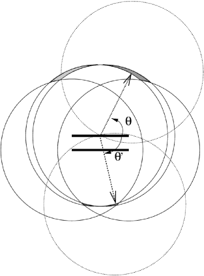
Figure 16: The loci of the centres of spheres contributing $\omega_{s}$ in the range $[\omega_{M}^{+}(1-\epsilon^{2}/2)$, $\omega_{M}^{+}[$. The dashed arrow points to a centre of such a sphere, and defines the running angle, $\theta$, mentioned in Eq. (113). The two (cylindrically symmetric) shaded regions correspond to the loci of the centre of spheres capturing almost half a ring and all or none of the other. Two examples of such spheres are displayed for either case.

C.2 the 3D statistics

The threshold on $\lambda_{\rm max}$, from which the caustics start to contribute at a given scale $R_{s}$ depends on the adopted description for the local vorticity. We assume here as mentioned in Sect. 4.3.2 that the total vorticity is localized on two rings of radius $e/3$ each, distant of $2\,d/3$ of each other. They are assumed to bear opposite lineic (and uniformly distributed) vorticities; in order to get a consistent answer for the integrated vorticity in a quadrant, we should have

$$\omega_{\rm lin.}={3\omega_{\rm quad.}\over e}.$$ (102)

The maximum vorticity that can be encompassed in a sphere then depends on its radius $R_{s}$. If $R_{s}$ is larger than the radius of the rings $e/3$, it is possible to have half of a ring in a sphere (while the other ring does not intersect it at all), so that the values of $\lambda_{\rm max}$ (for which the maximum vorticity is sampled) is given by

$$\omega_{s}={2\,e\,\omega_{lin.}\over 3}\,{1\over{4\pi\over 3}R_{s}^{3}}\equiv\omega_{M}^{+}={3\over 2\pi}\omega_{0}\,(\lambda_{\rm max}-1)^{\alpha}f(\Omega)\,{R_{L}^{3}\over R_{s}^{3}},\quad{\rm if}\quad R_{s}>e/3.$$ (103)

If on the other hand $R_{s}$ is smaller than $e/3$ then only a fraction of the half ring can be put in the sphere and we have instead

$$\omega_{s}={2\,R_{s}\,\omega_{lin.}}\,{1\over{4\pi\over 3}R_{s}^{3}}\equiv\omega_{M}^{-}={9\over 2\pi}\,{\omega_{0}\over e_{0}}\,(\lambda_{\rm max}-1)^{\alpha-\alpha_{e}}f(\Omega)\,{R_{L}^{2}\over R_{s}^{2}},\quad{\rm if}\quad R_{s}<e/3.$$ (104)

Now the local behaviour of $V_{\rm caus.}$ near its takeoff value is well represented (as argued below and demonstrated in Appendix D for large enough $R_{s}$) as a function of $\lambda_{\rm max}$ by

$$V_{\rm caus.}(R_{L},R_{s},\lambda_{\rm max},\omega_{s})=\int\Theta\left[\omega_{\bf c}\left({\bf c},R_{L},R_{s},\lambda_{\rm max}\right)-\omega_{s}\right]\,{\rm d}^{3}c\simeq R_{L}R_{s}^{2}V_{0}(\lambda_{\rm max}-\lambda_{\rm max}^{(0)})^{\gamma}\,,$$ (105)

Using Eq. (17) and  (52) for the distribution function $\ p_{\rm max}(\lambda_{\rm max})$, changing integration variable from $u=\lambda_{\rm max}/\sigma$ to $\lambda_{\rm max}^{(0)}+u/\lambda_{\rm max}^{(0)}$ and dropping the residual integral for large enough ${\lambda_{\rm max}^{(0)}/\sigma(R_{L})}$ (see Appendix E for details) yields for Eq. (95) :

$$P_{R_{s}}(>\omega_{s})\simeq\max_{R_{L}}\left[{6\,n_{0}\,V_{0}\Gamma(\gamma+1)\over 5^{\gamma+1}}\left({\lambda_{\rm max}^{(0)}\over\sigma(R_{L})}\right)^{4-\gamma}\ \exp\left[-{5\over 2}\left({\lambda_{\rm max}^{(0)}\over\sigma(R_{L})}\right)^{2}\right]{R_{s}^{2}\over R_{L}^{2}}\right],$$ (106)

From Eq. (22) and  (103),  (104), the minimum of the argument of the exponential corresponds to:

$${\lambda_{\rm max}^{+}\equiv{6\over 6-\alpha(n+3)}\quad{\rm if}\quad R_{s}>e/3},\quad{\rm and}\quad{\lambda_{\rm max}^{-}\equiv{4\over 4-(\alpha-\alpha_{e})(n+3)}\quad{\rm if}\quad R_{s}<e/3},$$ (107)

which assumes that $\alpha(n+3)<6$ (resp. $(\alpha-\alpha_{e})(n+3)<4$ ), both conditions being satisfied for all values of $n$ considered. The corresponding scaling relations between $R_{L}$ and $R_{s}$ are given by

$$R_{L}=f_{s}^{+}\ R_{s}\ \left({\omega_{s}\over f(\Omega)}\right)^{1/3}\quad{\rm if}\quad{R_{s}>e/3}\,,\quad{\rm or}\quad R_{L}=f_{s}^{-}\ R_{s}\ \left({\omega_{s}\over f(\Omega)}\right)^{1/2}\quad{\rm if}\quad{R_{s}<e/3}\,.$$ (108)

The scale factors $f_{s}^{\pm}$ – derived from the fits (Eq. (47)) – are given in Table (4) for an Einstein-de Sitter universe ($f(\Omega)=1$) and different values of $n$. Interestingly, as long as $\omega_{s}$ is not too large the condition $R_{L}>e/3$ is always satisfied. In practice at scales of about $10$ to $15h^{-1}$Mpc the measured vorticity $\omega_{s}$ is expected to be indeed at most of a few tenth (Bernardeau & van de Weygaert, 1995). It is therefore always fair to assume that we are in the régime where $R_{s}>e/3$ which is the régime investigated hereafter.

Completing the calculation of $P_{R_{s}}(>\omega_{s})$ requires evaluating the corresponding $n_{0}$, $\gamma$ and $V_{0}$. The value of $n_{0}$ is entirely determined by the geometry of the caustics and is given in the Tables 1 and 2. The behaviour of $V_{\rm caus.}$ as it departs from zero as a function of $\omega_{s}$ for the critical ratios of $R_{s}$, $e$ and $d$ is locally well fitted as a function of $\omega_{s}$ by a power law of the form

$$V_{\rm caus.}(\lambda_{\rm max},\omega_{s})\simeq U_{0}\ R_{L}\,R_{s}^{2}\left(1-{\omega_{s}\over\omega_{M}^{+}(\lambda_{\rm max})}\right)^{\gamma}\ \,.$$ (109)

where $\omega_{M}^{+}$ is the threshold value of $\omega_{s}$ (Eq. (103)). This expression is valid when $\omega_{s}$ is close to its threshold value. On the critical line, $\omega_{s}=\omega_{M}^{+}$, it is possible to relate the variation of $\lambda_{\rm max}$ to the variations of $\omega_{s}$. We can then rewrite Eq. (109) as a function of the difference between $\lambda_{\rm max}$ and the critical value $\lambda_{\rm max}^{(0)}$, assuming this departure is small,

$$V_{\rm caus.}(\lambda_{\rm max},\omega_{s})\simeq R_{L}\,R_{s}^{2}V_{0}\,(\lambda_{\rm max}-\lambda_{\rm max}^{(0)})^{\gamma}\ \,,\quad{\rm with}\quad V_{0}={U_{0}\,\alpha^{\gamma}\over(\lambda_{\rm max}^{(0)}-1)^{\gamma}}\ \,.$$ (110)

Since $R_{L}/R_{s}$ is only a function of $n$ and $\omega_{s}$, so are $V_{0}$ and $\gamma$. In practice we take the asymptotic values of $V_{0}$ and $\gamma$ given in Appendix D and corresponding to the limit $R_{s}\ll R_{L}$. Putting Eq. (110) into Eq. (106), using Eq. (107) – (109) and  (115) yields for the vorticity distribution

$$P_{R_{s}}(>\omega_{s})=0.48n_{0}V_{0}\left({\lambda_{\rm max}^{(0)}\over\sigma(R_{s})}\right)^{7/2}\,f_{s}^{(13+7n)\over 4}\,\omega_{s}^{(13+7n)\over 12}\,\exp\left[-{5\over 2}\,\left({\lambda_{\rm max}^{(0)}\over\sigma(R_{s})}\right)^{2}\,f_{s}^{n+3}\,\omega_{s}^{(n+3)/3}\right]\,.$$ (111)

Equation  (111) is illustrated on Fig. (14) and discussed in the main text.

Appendix D Asymptotic behaviour of $V_{\rm Caust.}$ in 3D

For large enough $R_{s}$ we derive here an asymptotic analytic expression for $V_{\rm Caust.}$. Let us first estimate geometrically the volume in space contributing almost $\omega_{M}^{+}$ to $V_{\rm Caust.}$. The corresponding contribution is the sum of two volumes given by the shaded area in Fig. (16), corresponding to the loci of the centers of spheres which capture almost half a ring and not the other, or which capture completely one ring and almost half of the other. In the asymptotic limit, as $e/R_{s}\to 0$, the element of volume is an infinitely thin strip and both contributions become equal since $\theta\to-\theta^{\prime}$. The area corresponding to these loci can be evaluated algebraically as follow: let us call $\epsilon$ the projected ring segment by which a sampling sphere of radius $R_{s}$ fails to encompass a ring diameter $2e/3$; it follows that the ratio of $\omega_{s}$ to $\omega_{M}^{+}$, is given by

$${\omega_{s}\over\omega_{M}^{+}}=(1-{\epsilon^{2}\over 2})\,.$$ (112)

On the other hand, for a given direction for the sphere centre given by $\cos(\theta)\equiv\mu$, within the solid angle $2\pi{\rm d}\mu$, the volume element (encompassed by the two shifted spheres capturing $\omega_{s}$ in the range $[\omega_{M}^{+}(1-\epsilon^{2}/2)$, $\omega_{M}^{+}[$) is given by

$$\left({2e\over 3}\right)4\pi\,R_{s}^{2}\epsilon\sin^{2}\theta{\rm d}\theta=8\pi{e\over 3}R_{s}^{2}\epsilon{\sqrt{1-\mu^{2}}}\,{\rm d}\mu\,.$$ (113)

Summing over all possible directions (i.e. before intersecting the second ring) yields

$$8\pi{e\over 3}R_{s}^{2}\epsilon\int\limits_{\mu_{0}}^{1}{\sqrt{1-\mu^{2}}}\,{\rm d}\mu\,\equiv\,8\,\pi\,{e^{(0)}\over 3}R_{L}\,R_{s}^{2}\,\epsilon{\cal J},\quad{\rm where}\quad\mu_{0}=\left[1+{4{d^{(0)}}^{2}\over{e^{(0)}}^{2}}\right]^{-1/2}\,.$$ (114)

Accounting for the summation over the two configurations (half a ring captured or a full + one half ring captured), using Eq. (112) to eliminate $\epsilon$, we finally get for large enough $R_{s}$

$$V_{\rm Caust.}=16\sqrt{2}\pi R_{L}\,R_{s}^{2}\,{e^{(0)}\over 3}\,\left(1-{\omega_{s}\over\omega_{M}^{+}}\right)^{1/2}\,,\quad{\rm therefore}\quad\gamma_{\infty}={1\over 2}\quad{\rm and}\quad U_{0}^{\infty}=16\sqrt{2}\pi{e^{(0)}\over 3}\,{\cal J}\,.$$ (115)

Appendix E Rare event approximation

Consider an integral of the form

$${\cal I}=\int\limits_{a}^{\infty}x^{\beta}(x-a)^{\gamma}\exp(-bx^{2})\,{\rm d}x\,.$$ (116)

Changing variable to $x=a+u/(2ab)$ Eq. (116) reads

$${\cal I}={1\over 2ab}\exp(-ba^{2})\int\limits_{0}^{\infty}\left({u\over 2ab}\right)^{\gamma}a^{\beta}\left[\left(1+{u\over 2a^{2}b}\right)^{\beta}\exp\left(-{u^{2}\over 2ba^{2}}\right)\right]\,\exp(-u)\,{\rm d}u\,.$$ (117)

For large enough $a$ the square brace in Eq. (117) is well approximated by $1$ yielding for Eq. (117)

$${\cal I}={a^{\beta-\gamma-1}\over(2b)^{\gamma+1}}\Gamma({\gamma+1})\,\exp(-ba^{2})\,.$$ (118)

Eq. (97) is a special case of Eq. (116) with $x=\lambda_{\rm max}/\sigma$, $a=\lambda_{\rm max}^{(0)}$, $\gamma=0$, $\beta=3$ and $b=4/3$, while Eq. (106) corresponds to $\beta=5$, and $b=5/2$. Note that the $\gamma=0$ approximant can be deduced directly by integration by parts.

References

- [bbks] Bardeen J.M., Bond J.R., Kaiser N., et al. 1986, ApJ, 304, 15
- [ Bernardeau (1994a)] Bernardeau F. 1994a, ApJ, 427, 51
- [Bernardeau, et. al. (1995)] Bernardeau F., Juszkiewicz R., Dekel A., Bouchet F.R. 1995, MNRAS, 274, 20
- [] Bernardeau F., Van de Weygaert R. 1996, MNRAS, 279, 693
- [bert85] Bertschinger E. 1985, ApJS, 58, 39
- [ Bertschinger (1989)] Bertschinger E., Dekel A. 1989, ApJ, 336, L5
- [ Bertschinger (1990)] Bertschinger E., Dekel A., Faber S.M., et al. 1990, ApJ, 364, 370
- [Bond 1987] Bond J. R., Efstathiou G. 1987, MNRAS, 226, 655
- [cat1] Catelan P., Theuns T. 1996, MNRAS, 282, 455
- [cat2] Catelan P., Theuns T. 1997, MNRAS, 292, 225
- [cou] Couchman, H. 1991, ApJ, 368L, 23
- [ Dekel (1994)] Dekel A. 1994, ARAA, 32, 371
- [ Dekel (1994)] Dekel A., Rees M. 1994, ApJ, 422, L1
- [Doroshkevich] Doroshkevich A.G. 1970, Astrofizika, 6, 581
- [eke] Eke V.R., Cole S., Frenk C.S. 1996, MNRAS, 282, 263
- [fillmore] Fillmore J.A., Goldreich P. 1984, ApJ, 281, 1
- [fisher] Fisher K.B., Davis M., Strauss M.A., Yahil A., Huchra J.P. 1993, ApJ, 402, 42
- [henry] Henry J.P., Arnaud K.A. 1991, ApJ, 372, 410
- [ Juszkiewicz (1995)] Juszkiewicz R., Weinberg D.H., Amsterdamski P., Chodorowski M., Bouchet F.R. 1995, ApJ, 442, 39
- [ Nusser (1993)] Nusser A., Dekel A., 1993, ApJ, 405, 437
- [ouk] Oukbir J., Blanchard A. 1997, A&A, 317, 1O
- [ Peebles (1980)] Peebles, P.J.E., 1980, The Large-Scale Structure of the Universe, Princeton Univ. Press
- [peack] Peacock J.A. 1991, MNRAS, 253, 1p
- [web] Pogosyan D., Bond J.R., Kofman L., Wadsley J. 1996, AAS, 189, 1303
- [press] Press W.H., Schechter P.L. 1974, ApJ, 187, 425
- [melott] Splinter R.J., Melott A.L., Shandarin S., Suto Y., 1998, ApJ, 497, 38
- [steinmetz] Steinmetz M., White S. 1997, MNRAS, 288, 545
- [suisalu] Suisalu I., Saar E. 1995, MNRAS, 274, 287
- [white 1] White S.D.M. 1984, ApJ, 286, 38