Nonuniqueness and Structural Stability
of Self-Consistent Models of Elliptical Galaxies
By
Christos Siopis
A DISSERTATION PRESENTED TO THE GRADUATE SCHOOL
OF THE UNIVERSITY OF FLORIDA IN PARTIAL FULFILLMENT
OF THE REQUIREMENTS FOR THE DEGREE OF
DOCTOR OF PHILOSOPHY
UNIVERSITY OF FLORIDA
1999
Dedicated with love to my parents, Vassili and Maria, and to
my sister Eleni
for all their support, encouragement and
understanding
ACKNOWLEDGEMENTS
It takes a certain amount of perseverance, love for one’s research subject, and, sometimes, some dose of insanity, to pursue a doctoral degree. This highest of scholar degrees with which mankind awards individuals, is usually the culmination and convergence point of most of the candidate’s previous plans and goals in life, and often takes a lifetime of preparation to achieve. For this reason, I would like to thank all the wonderful people who helped nurture my interest in science, and learning in general, during my pre-college years, and especially my parents, to whom this dissertation is dedicated. They always encouraged me to follow my dreams and never attempted to interfere except to help me achieve them, even if that meant that they would have to sacrifice or alter some of their plans and expectations, and for that I am grateful.
I would like to express my gratitude to my college professors at the University of Ioannina, Greece, and especially Drs. I. E. Lagaris, E. Manesis and V. Tsikoudi, for showing genuine interest and helping me achieve my goal of pursuing a graduate degree. I am particularly indebted to Dr. Tsikoudi, my undergraduate professor of Astronomy, who encouraged my aspirations for a graduate degree throughout my college years, then spent endless hours working with me, helping me make crucial decisions during the hectic months before graduate application deadlines, and supported me and my family when the time had come to leave home and change continent. It is no exaggeration to say that most probably this dissertation would not have even started without her personal involvement and support, and I would like to let her know that they are truly appreciated.
It would be a grave omission not to express my gratitude to our family friends, Leonidas Gkelios, a former Air Force and civil aviation pilot, and his wife, Agni. Their travel experience, tips and advice, but most of all their moral support to me and my parents during the days before my departure for the United States and the first weeks thereafter, were invaluable and will be forever remembered and appreciated.
It is hard for me to imagine that I could have been more fortunate than having Henry Kandrup as my advisor. Henry masters an impressive combination of breadth and depth of knowledge and experience that make him an invaluable resource for a graduate student. At the same time, he shows a deep respect and personal interest for his students, being always available, never “too busy,” ready to provide his insight whenever needed, but in such a way that the student will come to realize, on his or her own, where the error or the problem was, and learn from it. He works closely with his students to establish what they really want to do —occasionally altering his own research plans to accommodate their interests— and making it clear all along, in a nonverbal but very obvious way, that it is the student, and not some narrowly defined project, what matters most. This experience has been quite overwhelming, and I can only hope that one day I can show my true appreciation and gratitude by imitating just a few of these virtues.
It is a great pleasure to acknowledge the close collaboration, for parts of this dissertation, with Dr. E. Athanassoula of the Observatoire de Marseille, France. I am indebted for her hospitality and financial support during my two-month stay at the observatory, but also for the lengthy discussions and constructive criticisms that have strengthened the credibility of the results reported in this work. Access to her group’s GRAPE computer facility is instrumental for the ongoing structural stability studies, briefly described in Chapter 4, but also for pointing out the necessity of studying the simpler case of a Plummer sphere, in Chapter 2.
Professor George Contopoulos has certainly been along with me during this scientific journey for longer than anyone else. His astronomy lecture notes, from the time when he was at the University of Thessaloniki, Greece, helped nourish my fledgling interest in astronomy (even unknowingly to him) during my high-school years, and the lectures and discussions he has had with me years later, as a visiting professor at the University of Florida, helped better shape the goals of this research. But I am also thankful to him and to the European Community Human Capital and Mobility program for offering me the opportunity to spend part of a summer at the Institut für Astronomie of the University of Vienna, Austria, in collaboration with Dr. Rudolf Dvorak, working on a project that would give me a better understanding of short-time Lyapunov exponents, a tool that proved particularly useful in parts of this dissertation. Very special thanks should go here, of course, to a wonderful Rudi Dvorak, for all the discussions, the useful comments and the encouragement that he offered, and for his outstanding hospitality.
At the heart of this research project lies the quadratic programming method that solves the optimization problem and computes the models on which most of the conclusions of this work are based. I am truly indebted to Dr. Cs. Mészáros of the MTA SZTAKI Computer and Automation Research Institute of the Hungarian Academy of Sciences, who generously made available, free of charge, recent versions of his quadratic/linear programming solver, BPMPD, and spent his time answering my questions. BPMPD is a fine piece of software, robust and very efficient in its use of computational resources. Without BPMPD, the scope and credibility of this work would be severely restricted.
Brent Nelson, our computer systems administrator, was at the receiving end of much of the heat related to this project and he deserves special thanks. If it were not for his far-sighted strategy of installing a cost-effective, powerful and versatile cluster of Linux workstations, the quality of this work would have been severely compromised.
I would also like to thank all of my committee members for their interest and support, and especially Drs. Haywood Smith, for his careful reading of the manuscript and his suggestions; Jim Ipser, for the time that he spent for me on a number of occasions and for his advice; and Steve Gottesman and his wife Mariou for their interest and encouragement, on academic as well as culinary and other matters. It is also a pleasure to thank Dr. Robert Wilson for his hospitality on a number of occasions, and Dr. Heinrich Eichhorn for several discussions on issues related to my research, but also on a wide range of other topics.
During the years of this work, I have been the beneficiary of advice and encouragement from a number of people who have done work in this field and on whose work my research was largely based. I would like to thank Dr. David Merritt for providing much of the motivation for doing this work, and for useful discussions and advice on a number of implementation and conceptual issues that he kindly offered me on a number of occasions; and Drs. Chris Hunter, Tim de Zeeuw and Ron Buta for encouragement and helpful advice.
It is also a great pleasure to acknowledge the help and friendship of a number of former graduate students (and now doctors) in my department. First, I would like to thank Dave Kaufmann for many lively discussions, especially on the Contopoulos-Grosbøl method for constructing self-consistent models of galaxies —a great help during my first steps in this project from a veteran galaxy builder; Seppo Laine for being so obligingly helpful, especially during my first year of adaptation to life in Gainesville, and for all the adventures that we have been to thereafter; Jaydeep Mukherjee, for being such a great friend, counselor and mentor; and Dimitri Pourbaix, for his obliging assistance with a number of numerical analysis and computer-related problems, as well as for the endless pleasure of debating with him on any and all issues.
Thanks to the vigilance of our three office ladies, Ann Elton, Glenda Smith and Debra Hunter, many administrative pitholes were averted and others were promptly remedied. Their assistance, care and smiling faces are appreciated.
The financial and moral support of the Department of Astronomy is also gratefully appreciated. Furthermore, I would like to acknowledge a Fulbright Fellowship that greatly facilitated my first year of graduate studies, a Research Assistantship from the Florida Space Grant Consortium (NASA), and a Sigma-Xi Grant-in-Aid of Research which was essential in allowing me to travel to Marseille.
Finally, I would like to thank the people of Florida and of the United States for their hospitality and accommodation during my years of study at the University of Florida.
TABLE OF CONTENTS
toc
Abstract of Dissertation Presented to the Graduate School
of the University of Florida in Partial Fulfillment of the
Requirements for the Degree of Doctor of Philosophy
Nonuniqueness and Structural Stability
of Self-Consistent Models of Elliptical Galaxies
By
Christos Siopis
May 1999
Chairman: Dr. Henry E. Kandrup
Major Department: Astronomy
Schwarzschild’s method was used to construct equilibrium solutions to the collisionless Boltzmann equation corresponding to a Plummer sphere. These solutions were compared with analytical results to test the robustness of the numerical method and its efficiency in probing the degeneracy of the solution space. The method was then used to construct genuinely triaxial stellar equilibria, for which no analytical solutions are known, and to study their nonuniqueness. The particular model that was studied is a three-dimensional generalization of Dehnen’s spherical potential, which contains a central density cusp and admits both regular and chaotic orbits. It was found that, for a model with a weak density cusp, self-consistent models do not exist if the chaotic orbits are assumed to be completely mixed so as to yield a time-independent building-block: only the innermost 65% of the mass can be mixed. In these inner regions, it is possible to obtain alternative solutions that contain significantly different numbers of chaotic orbits, yet yield (at least approximately) the same mass density distribution. However, it is not clear whether these solutions are truly time-independent, since the “unmixed” chaotic orbits in the outer regions, which do not sample an invariant measure, can cause secular evolution. When using Schwarzschild’s method, one must be very careful to sample accessible phase-space as comprehensively and as densely as possible, while at the same time ensuring that each orbit is a truly time-independent building block. Some of the numerical equilibria were sampled to generate initial conditions for -body simulations, with the aim of testing the structural stability of the models. Preliminary work showed that no catastrophic evolution takes place, but there is a weak tendency for the configuration to become more nearly axisymmetric over a period of several dynamical times. It is not presently clear whether this tendency is real or a numerical artifact.
Chapter 1 INTRODUCTION AND MOTIVATION
1.1 Some Preliminaries about Galaxies
The research field of galactic dynamics was arguably born when Edwin Hubble established in 1923 that William Parsons’ “spiral nebulae,” a subset of objects from William Herschel’s extensive catalog of nebulae, were in fact gigantic conglomerations of stars, like the Milky Way galaxy. They were thus appropriately called “galaxies,” and the Milky Way was demoted to a mere sample in a universe filled with billions of peer galaxies – though its initial letter was now capitalized and promoted to “the Galaxy.” Most galaxies lie at such enormous distances that only the combined glow of their billions of stars can be detected. This explains why, until 75 years ago, they were confused with the visually similar soft glow of emission nebulae in the Galaxy.
Galaxies come in a variety of shapes, sizes and masses. In terms of their appearance, they are classified as spiral, elliptical and irregular, based on the morphological classification scheme introduced by Hubble (1936). Spiral galaxies come in two flavors, normal and barred (although there is mounting evidence that most spirals are barred, with only the size of the bar varying among them). In order of increasing tightness of the winding of their spiral arms, spirals are classified as S(B)c, S(B)b or S(B)a, as well as S(B)0 (or lenticular) when they exhibit a central bulge but no identifiable spiral arms. The letter B is included when the spiral is barred.
Ellipticals are designated E, where and is the axial ratio of their projected brightness ellipsoid. The index ranges from 0 for round ellipticals to 6 for highly elongated ones. Very few, if any, ellipticals are more elongated than E6, for reasons that seem to be related to dynamical instabilities that grow with increasing ellipticity (cf. e.g., Merritt and Stiavelli, 1990; Merritt and Hernquist, 1991). It should be noted that, whereas the spiral sequence S0-Sa-Sb-Sc correlates, at least roughly, with significant physical quantities (for instance, the importance of dynamical rotation increases, compared to random motions, from S0 to Sc), this does not seem to be the case with the elliptical E0-E6 sequence, where variations in apparent ellipticities must be mainly a result of projection effects. However, one can still extract some important conclusions from the statistical manipulation of the projected axial ratios of elliptical galaxies.
It is useful to keep in mind that the E subclassification scheme is not as well-defined and consistent as one might think, mainly due to inadequacies of the photographic techniques that were used for the classification of most elliptical galaxies. For example, different workers used the axis ratios of different isophotes to determine . Furthermore, more detailed observations have revealed quite early on that the ellipticity of the isophotes can change with radius (cf. e.g., Redman and Shirley, 1938; Liller, 1960, 1966; Carter, 1978), leading to the inconvenience that the subclassification of a given elliptical may change as a function of the position, along the semimajor axis, where the ellipticity is determined. Therefore, the index should only be taken as a visual indication of ellipticity measured at a “moderately faint” isophote.
Another effect that is not taken into account in the E subclassification is the occurrence of isophote twists, i.e., variations with radius of the position angles of the major axes of the isophotes. Evidence for this effect, which is present in many ellipticals, started accumulating early on (cf. e.g., Evans, 1951; Liller, 1960; Carter, 1978; Williams and Schwarzschild, 1979). Both variations in ellipticity and in position angle were confirmed and studied in detail with subsequent CCD observations.
More recently (Kormendy and Bender, 1996; Tremblay and Merritt, 1996), some consensus seems to be developing among workers that, based on physically significant criteria, most elliptical galaxies fall into one of two categories. In the first category belong normal- and low-luminosity, rapidly rotating, nearly isotropic, oblate-spheroidal ellipticals, which can be morphologically distinguished for being coreless and for having disky-distorted isophotes. In the second category belong giant, essentially non-rotating, anisotropic and moderately triaxial ellipticals that have cuspy cores and boxy-distorted isophotes (by “triaxial” these authors mean that the equidensity surfaces in the outer parts of the galaxies are non-degenerate ellipsoids, i.e., ellipsoids with three different semi-axes ; see §1.4.1 for more on triaxiality and elliptical galaxies). This dichotomy, if true, could also imply different formation processes for the two categories of ellipticals. For example, it is tempting to suggest that triaxial slow rotators are the remnants of galactic mergers, whereas the spheroidal, flattened, fast rotators formed via dissipative processes and are perhaps continuously linked to the S0 type of disk galaxies that show no spiral structure.
Concerning now the masses of galaxies, if the galaxian mass distribution in the Local Group of galaxies is typical, then dwarf galaxies with masses (such as the irregular Magellanic Clouds, or M32, the dwarf elliptical companion of the Andromeda galaxy) should outnumber the normal galaxies with (such as the Galaxy and M31, the Andromeda galaxy) by at least an order of magnitude. The most massive galaxies () are the central dominant (cD) galaxies that reside near the centers of many clusters of galaxies. Notwithstanding the sheer numbers of dwarf galaxies and the large masses of cD galaxies, most of the luminous mass in the local universe probably resides in normal galaxies.
The luminous matter in galaxies consists mainly of stars, gas and dust. Stars are responsible for the overwhelming fraction of the luminous mass of most galaxies. In spiral galaxies, the contribution of gas and dust to the total mass is usually restricted to the few-percent level, although in some rare cases it can account for up to 10-20%. It might thus seem that, at least as far as dynamics is concerned, gas and dust play a marginal role for all but the most gas-rich spirals. Indeed, they are often treated as test particles, moving under the influence of the stellar gravitational background field.
However, this picture is not entirely accurate. Despite their relative sparsity, gas and dust play an essential role in star formation, the evolution of bars, the formation of spiral arms, and in other processes that rely on the dissipative properties of gas. The capability of gas to convert organized kinetic energy into random thermal motion via dissipation enables it to go to places where stars cannot go, because they are subject to Liouville’s theorem and their motion is restricted by the incompressibility of Hamiltonian flows. Gas can thus alter the mass distribution of a spiral galaxy over time and cause secular evolution. Furthermore, clumpy gaseous structures, such as giant molecular clouds, often present fairly substantial gravitational cross-sections that can scatter stars much more effectively than star-star encounters, thus “heating” disk stars (i.e., increasing the velocity dispersion of the disk population) and accelerating phase-space transport. The upshot is that, depending on the particular problem at hand, it may or may not be safe to ignore gas in a dynamical study of spiral galaxies.
The situation is quite different for elliptical galaxies. Until less than two decades ago, it was widely believed, on the basis of optical observations, that ellipticals contain very little gas and dust. Since then, X-ray observations have established the presence of substantial amounts of hot ( K) gas (cf. e.g., Fabbiano, 1989, and references therein). In fact, the gas-to-star mass ratio in ellipticals seems to be comparable to that in spirals, though in the latter it is found mostly in warm ( K ionized gas) and cold ( K atomic and molecular gas) conditions. Ellipticals also contain warm and cold gas, as well as dust, but their quantities are almost negligible. In fact, most cases of substantial warm/cold gas and/or dust detections have been reported for ellipticals that are morphologically classified as peculiar. Furthermore, in these cases, the cold gas and dust often appear to be kinematically decoupled from the stellar population. This evidence suggests that cold gas and dust must have an external origin, such as mergers with gas-rich companion galaxies (cf. e.g., Bregman et al., 1992, and references therein).
Despite the fact that elliptical galaxies possess a rich and complex interstellar medium, which is still not very well understood, its effect on the dynamics of its host galaxy is expected to be all but negligible, given the low fraction of the total mass that it represents. Furthermore, the Jeans mass associated with gas at such high temperatures is so large that gas cannot collapse to form stars. In general, the high virial temperature of the gas prevents it from forming clumps and substructures that could affect the dynamics of ellipticals in ways similar to the ones described above for spirals. Instead, the interstellar gas of elliptical galaxies acts more like a backdrop against which stellar dynamics unfolds, and is therefore safe to ignore in most dynamical studies.
The preceding discussion concerned the luminous matter in galaxies and ignored their content in dark matter, the purported substance out of which as much as 90-99% (or even more, according to some estimates) of the mass of the universe is made, but which emits no detectable electromagnetic radiation. Its presence is only inferred from its gravitational effects on visible matter. These effects are most important over cosmological and intergalactic distance scales, although they can also affect the internal dynamics of galaxies. For example, the presence of massive dark halos surrounding disk galaxies may play a major role in the formation and strength of disk warps, bars and other structures. The effects of dark matter on elliptical galaxies are less clear (cf. e.g., Stiavelli and Sparke, 1991).
Nevertheless, the very fact that dark matter emits no detectable amounts of electromagnetic radiation strongly suggests that it is non-dissipative in nature. This, in turn, implies that (a) it clumps less than luminous matter, and thus it might not dominate the dynamics of galaxies that presumably live near the bottom of the gravitational well created by the dark matter, and (b) to the extent that dark matter does influence the dynamics of luminous matter, at least the dynamics is still Hamiltonian. In other words, if one assumes galactic matter is collisionless, whether it is dark matter or stars is nearly irrelevant.
The research presented in this dissertation was conducted without taking dark matter into account. This was done not because it is dynamically unimportant, although for the kind of questions posed here it may well be, but (i) because current understanding of the dark matter problem is quite incomplete, thus making it hard to correctly incorporate it in this dynamical study; and, more importantly, (ii) because the aim of this work, as explained in §1.4, is to develop a better understanding of certain generic physical processes that may be taking place in elliptical galaxies, irrespective, to a certain extent, of the specific form of their gravitational potentials –so long as the collisionless, Hamiltonian approximation remains valid. For the same reason, no reference will be made to the effects of varying mass-to-light ratios, which can be important if one studies the dynamics of a specific object. However, there is still a potential concern, namely that stars and dark matter could evolve differently as they approach equilibrium, especially if the dark matter is made of very low-mass fermions which cannot clump on short scales. But allowing for such degeneracy is outside the scope of this work.
Finally, it should be noted that the preceding discussion refers to galaxies in the local universe. At times that correspond to redshifts of or so, most of the matter in galaxies was still in the form of gas, and gas dynamics played a much more important role. Peculiar and irregular galaxies were more common and, especially at still higher ’s, galactic collisions were more common as well. A collisionless, nearly-time-independent approach to galactic dynamics would presumably not be particularly fruitful at those times.
The following section is a brief overview of the mean field theory and the collisionless Boltzmann equation, the foundations for the statistical treatment of dissipationless self-gravitating systems of many bodies. Solving the collisionless Boltzmann equation is the topic of §1.3, followed by a discussion of the outstanding problems that motivated this work and an overview of the dissertation in §1.4.
1.2 The Collisionless Boltzmann Equation and the Mean Field Approximation
Let the probability of a given ensemble of stars, that represents the density distribution of a galaxy, at a given time be
| (1.1) |
so that , where , represents the joint probability that star be found inside the phase-space volume element centered around , simultaneously for all at time . This implies that is normalized so that , which is feasible since it is a realistic expectation for galaxies that as and (there is a finite number of stars in a galaxy).
If there are no sources or drains of stars in the system, then conservation of probability and the incompressibility of the flow dictate that
| (1.2) |
where for any vector , and denotes the inner product. However, from the equations of motion for a self-gravitating system of point masses one obtains
| (1.3) |
and
| (1.4) |
where is the two-body potential, and is the mass of individual stars in the system, which is assumed to be the same for all stars. This assumption imparts no loss of generality within the context of a mean field approximation (see below in this section), where stars are treated as zero-mass test particles moving under the influence of the bulk field.
Even though is the fundamental statistical object, it is an -particle distribution function (DF) that cannot be directly compared to any observables. Of more interest in that respect would be the one-particle DF
| (1.5) |
that provides the probability of finding particle near , irrespective of the positions and velocities of the other stars in the system. Substitution of Eqs. (1.2), (1.3) and (1.4) into (1.5) and integration by parts (remembering that as and and that all particles are assumed to be identical) gives
| (1.6) |
where
| (1.7) |
is the two-particle DF. In other words, the evolution of the one-particle DF requires knowledge of the two-particle DF, and in general the evolution of the -particle DF requires knowledge of the -particle DF, all the way up to (BBGKY hierarchy). This inability to decouple local from global dynamics is a consequence of gravity being a long-range force. Some progress can be made by writing
| (1.8) |
where reflects the degree to which stars and are correlated. In general, , i.e., the probability of finding particle near depends on the probability of finding particle near . Substitution of Eq. (1.8) into (1.6) yields
| (1.9) |
where
| (1.10) |
is the mean potential energy associated with the average forces acting on particle , and the right hand side describes the evolution of the one-particle DF caused by particle-particle correlations.
If it is valid to approximate , then Eq. (1.9) becomes the collisionless Boltzmann equation (CBE) (also known as the Vlasov equation in plasma physics, but see as well Hénon, 1982):
| (1.11) |
where the indices have been dropped for convenience since all the particles are considered to be identical, is the velocity of the particle, and
| (1.12) |
is the potential energy (this implies the normalization ).
Setting is called the self-consistent field approximation. This mean field theory approach, that led to the CBE, is a conceptually important tool that enables the worker to neglect direct particle-particle interactions, which can be hard to model, and describe the evolution of a particle solely as a result of its interaction with the bulk gravitational field. The most important consequence of this simplification stems from the fact that the CBE can be shown to be a (noncanonical) Hamiltonian system, , where the fundamental variable is itself and represents the mean field energy (Morrison, 1980; Kandrup, 1990a):
| (1.13) |
Clearly, then, it is important to investigate whether and when the assumption that is a valid and realistic approximation.
Chandrasekhar (1943b), in his classic monograph “Principles of Stellar Dynamics,” considered the gravitational Rutherford scattering of a test star moving in an idealized infinite and homogeneous distribution of point stars. By symmetry, there is no net force acting on the test star due to the bulk gravitational field of the system, so that, in the absence of “close” encounters with other stars, it would simply move at a constant velocity. However, random stellar encounters do occur and they have the effect of altering the velocity and the energy of the test star. In a real galaxy all stars obviously participate in this process, which leads to a secular evolution towards, albeit not to, a “relaxed” state of local thermodynamic equilibrium, characterized by a Maxwellian, isothermal distribution of stellar velocities (Kandrup, 1985). The relaxation time, , is then defined as the time needed for the cumulative effects of stellar encounters to alter the orbit of the test star to such an extent that the mean field approximation breaks down, meaning that the star cannot be considered as an independent, conservative dynamical system any more. This could be quantified, for example, by the time needed for the root-mean-square (rms) energy changes suffered by the test star as a result of the encounters to become comparable to its total energy.
An alternative approach, also pioneered by Chandrasekhar (1943a), treats stellar encounters as a stochastic process, and is a typical example of the fluctuation-dissipation theorem. There are three ingredients in this picture:
-
•
The bulk gravitational potential, , that determines the motion in the absence of any stellar encounters.
-
•
A systematic diffusion in velocity space, modeled as a sum of “random kicks” experienced by the test star due to its encounters with other stars. These can be seen as random force () fluctuations overimposed to the bulk mean field. They have the effect of pumping kinetic energy into the test star by increasing its rms velocity. is usually idealized as a delta-correlated Gaussian random process with zero mean (). Delta-correlation means that the forces at times and are uncorrelated, whereas Gaussian statistics means that the process is characterized completely by its first two moments. Therefore, everything about is encapsulated in the two-point correlation function , where the superscripts indicate spatial components, and the terms and respectively express the fact that the force is time-uncorrelated, and that its vector components in different directions are also uncorrelated. The proportionality coefficient will be specified below.
-
•
A systematic dynamical friction, , antiparallel to the direction of motion, that has the effect of continuously decelerating the test star along its direction of motion. Dynamical friction can be understood qualitatively by considering the test star moving with velocity in the surrounding medium and creating a “wake” of stars behind it. The wake corresponds to an excess density of stars behind the moving test star, and the gravitational force associated with it will tend to decelerate the test star along its direction of motion. In other words, dynamical friction has the effect of removing kinetic energy from the test star and heating up the surrounding medium. The coefficient , which has units of inverse time (see Eq. 1.14 below), scales as , This is not surprising since both and reflect the effects of graininess induced by the fluctuations and should be characterized by similar time scales.
These three ingredients interact according to a Langevin-type equation:
| (1.14) |
where, from the preceding discussion, it follows that the random force must obey
| (1.15) |
Here is the characteristic temperature (or mean squared velocity) associated with .
It is important to assess the effects of collisionality in the study of stellar systems: considering the complications introduced by taking it into account, it would be useful to see if there are cases where it can be dismissed. The first question to ask then is what the time scale of relaxation is. From the preceding discussion it becomes apparent that there are a number of ways for defining , but they are all associated by the same physical process and, quite reassuringly, they all lead to the same functional form and similar numerical values for (Chandrasekhar, 1943b):
| (1.16) |
where is the characteristic stellar speed, is the characteristic size of the system, and is the number of stars it contains. If the system is in approximate virial equilibrium, then , in which case the last equation becomes
| (1.17) |
where is a typical dynamical, or crossing, time for the system.
The second question to ask is how important collisionality is in a realistic stellar system. In the case of relatively small stellar systems, such as globular clusters with stars and yr, stellar collisions may be important over a cluster’s typical lifetime of yr. However, for galaxies with stars and years, the relaxation time is several orders of magnitude longer than the age of the universe. This has been customarily interpreted (cf. e.g., Binney and Tremaine, 1987, p. 190) as implying that stellar encounters are entirely unimportant and that the collisionless Boltzmann equation is an adequate description of the dynamics. However, this may not always be the case and collisional effects may be important in relation to the question of structural stability of galaxies (Pfenniger, 1986; Habib et al., 1997).
1.3 Solving the Collisionless Boltzmann Equation
1.3.1 Time-Dependent Solutions
Analytical solutions. The time-dependent CBE (1.11) is a seven-dimensional partial differential equation. Generic analytical solutions are only known for highly idealized systems, systems of lower dimensionality and for special cases (cf. e.g., Talpaert, 1975; Louis and Gerhard, 1988; Sridhar, 1989; Carrillo et al., 1996; Davidson, 1990, and references therein)
However, it is still possible to extract useful information from the CBE analytically, by calculating moments of the equation. Thus, for example, by integrating Eq. (1.11) over all possible velocities one obtains the zeroth-order moment, which is a continuity equation in configuration space:
| (1.18) |
where is the configuration-space density of the system and is the mean value of the th component of the velocity. Similarly, by multiplying Eq. (1.11) by and integrating over all velocities, one obtains the first-order moment, which is the analog of Euler’s equation for stellar dynamics:
| (1.19) |
where is the symmetric stress tensor, the analog of pressure () for fluids. The utility of these two relations, which are called the Jeans equations, should now be obvious: even though they contain less information than the CBE itself, they describe observable quantities, such as density, mean velocity and velocity dispersions, thus enabling, at least in principle, comparison with observations (cf. §1.3.2). A number of problems in stellar dynamics have been addressed via the Jeans equations (cf. e.g., Binney and Tremaine, 1987, pp. 198 - 211).
There is no reason why higher order moments cannot be computed. In fact, it might at first seem possible to distill much of the information contained in the CBE by considering a coupled set of moments equations, truncated to some appropriately high order. This is indeed a viable option (see “numerical solutions” below) but it turns out that every moment equation of a given order contains dispersion terms that can only be computed by a moment equation of the next higher order (for example, involves that can only be computed via a second-order moment equation). This is unlike the case with fluid dynamics, where an equation of state, , allows one to truncate the hierarchy by providing a relation between local pressure and density. Such an equation of state reflects the fact that perfect fluids are collision-dominated, so that one can assume local thermal equilibrium. By contrast, self-gravitating systems like galaxies are presumed to be nearly collisionless (this is why, for example, it makes sense to identify an anisotropic pressure tensor for equilibrium solutions to the CBE). Thus an infinite system of moment equations is needed to describe all the information contained in the CBE. However, it is still possible to make use of moment equations by truncating the infinite series via some assumption about the form of . Obviously, the validity of this approximation depends on the validity of the assumption.
Numerical solutions. In order to study more realistic systems one has to resort to numerical simulations. Unfortunately, solving the full-fledged seven-dimensional equation is so taxing in terms of computer speed and, even more so, memory requirements that only very recently is it becoming feasible to use grids that are large enough to attack realistic problems in three degrees of freedom. Nevertheless, there are a number of numerical solvers for one- and two-dimensional problems (cf. e.g., Cheng and Knorr, 1976; Yabe and Aoki, 1991; Yabe et al., 1991; Syer and Tremaine, 1995; Hozumi, 1997; Utsumi et al., 1998, and references therein).
Another possibility is to work with moments of the CBE, in the spirit of
the discussion earlier in this section. The object now is to numerically
solve a truncated set of coupled moments equations, with the caveats that
were given above. Such work has already been done to test stability in
plasmas (Channell, 1995) and extensions to track nonlinear evolution are
under way, both in plasmas and in self-gravitating systems, at Los Alamos
National Laboratory (Habib et al., in progress).
1.3.2 Time-Independent (Steady-State) Solutions
The aim here is to find time-independent (or steady-state or stationary or equilibrium) solutions to the CBE, i.e., solutions that satisfy in some coordinate system. Eq. (1.11) then becomes
| (1.20) |
where, as before, is defined self-consistently via Poisson’s equation:
| (1.21) |
Despite the superficial similarity between Eqs. (1.11) and (1.20), the process of finding stationary solutions is very different from that of solving the time-dependent CBE that was discussed in the previous section. In that case, the task was to compute the evolution in time, , of a DF that obeys the partial differential equation (1.11), for an arbitrary initial condition . The instantaneous form of the DF at time determines its form at , self-consistently via the potential.
By contrast, in the stationary problem, the task at hand is to find one or more time-independent, positive semi-definite functions that satisfy the integro-differential equation (1.20). The form of the function will have to be such that it will be able to support itself self-consistently. In other words, the potential will have to shuffle phase-space elements in such a way that no change will be imparted to . It should then come as no surprise that the existence of a self-consistent equilibrium corresponding to an arbitrary potential , or density distribution , is not guaranteed. Furthermore, if an equilibrium does exist, it may well not be the only one that exists, i.e., its uniqueness is not guaranteed.
Before proceeding to a brief overview of the techniques and tools available for the construction of equilibrium models of galaxies, there are two questions that should be addressed to investigate the legitimacy of using self-consistent equilibria as realistic approximations of galaxies.
1. Are galaxies in a state of equilibrium? If a galaxy is not in a state of equilibrium, then generally speaking, either (i) it would undergo a rapid (comparable to a characteristic crossing time) or even catastrophic evolution, or (ii) it would undergo a slow, secular evolution, or (iii) it would exhibit some kind of oscillatory behavior. The first possibility is easily ruled out. If galaxies were evolving rapidly, one would expect to observe a number of them at different stages of their evolution. However, with the exception of galaxies in the process of colliding, merging or having a close encounter with other galaxies, now or in the near past, most systems seem to have “regular” shapes, as evidenced by the relatively few Hubble types that are needed to classify most of them. Still, the second and third possibilities can certainly not be ruled out. Even though neither secular evolution nor oscillatory modes are directly accessible to observation, there is considerable theoretical and numerical evidence that they do occur. To name but a few examples, bars are believed to cause secular evolution in disk galaxies via redistribution of mass and angular momentum; cooling flows may be slowly altering the mass distribution near the central regions of elliptical galaxies; fast galactic flybys and the final stages of galactic mergers can trigger oscillatory modes that often persist long after the bulk of the interaction is over; and the presence of one or more companion galaxies or membership in a dense cluster of galaxies can induce a permanent quasi-periodic driving. These theoretical and numerical findings are often corroborated by indirect observational evidence, such as nuclear galactic starbursts, off-center galactic nuclei, the presence of decoupled kinematic components inside a galaxy, etc.
By contrast, the traditional approach to galactic modeling (cf. e.g., Binney and Tremaine, 1987, p. 4 and pp. 177-183) has been to assume that galaxies are in a state of quasi-equilibrium, and to use adiabatic invariance to treat the effects of a slowly-varying mean field due to secular evolution or long-period oscillations. This may be a good approximation for systems of one degree of freedom, for which adiabatic invariance was in fact shown, but not necessarily so for systems of more degrees of freedom, where the adiabatic theorem is weaker and actions may actually change faster than previously thought (Weinberg, 1994). Furthermore, if the galactic potential is strongly nonintegrable (cf. §1.3.2 under “Stellar Orbits”), resonant driving of chaotic orbits can induce changes in the distribution of energies and, hence, in the bulk distribution of matter, thus causing continuing evolution to the system (Kandrup et al., 1995).
Despite the evidence, very little has been done in terms of constructing time-dependent self-consistent models that reproduce the visual appearance of galaxies, though this may not be surprising in view of the difficulties involved in such a task. However, it can be argued that the study of stationary solutions to the CBE is still important, even as a first step towards an understanding of time-dependent systems. Furthermore, stationary solutions may still be useful approximations of quasi-stationary galaxies, provided at least that they are structurally stable, meaning that they are stable against perturbations that tend to alter the form of the potential. Examples of such perturbations include dynamical friction and noise due to stellar encounters (Eq. 1.14), periodic driving due to companion galaxies, or an impulse due to a fast galactic flyby. In other words, the motivation for structural stability analysis is the recognition that most probably galactic potentials do not have the exact form assigned to them by galactic dynamicists, and that therefore it is crucial to examine whether a particular model’s stability (and thus its usefulness, at least as a realistic approximation of a galaxy) strongly depends on small changes of the functional form of the potential. Again, very little has been done in terms of investigating the structural stability of self-consistent galactic models. Most work on this topic terminates with the construction of a time-independent DF. This dissertation will address some aspects of this problem (cf. §1.4).
2. Does the time-dependent collisionless Boltzmann equation guarantee convergence towards an equilibrium? Even if one assumes that galaxies today are in a state of quasi-equilibrium, they have not always been that way. They had to form and evolve to their present state. Despite the fact that the process of galaxy formation is not well understood, it is clear that after a certain stage in the life of ellipticals, gas dissipation becomes unimportant and, since then, their evolution is determined by the CBE. One might therefore attempt to answer the previous question, i.e., whether galaxies are in a state of equilibrium, by investigating whether the time-dependent CBE dictates an evolution towards a nearly time-independent final state.
The basic point here is that, because the evolution described by the CBE is Hamiltonian, the DF cannot reach a state of equilibrium in a pointwise sense. If is nonzero, it will remain nonzero and the evolution will lead to phase mixing, since the flow is incompressible and CBE characteristics do not cross. Nevertheless, it is often assumed that the CBE somehow approaches equilibrium in some appropriate coarse-grained sense. However, there is no proof that such is the case. Rather, the only result known to date regarding the asymptotic time behavior of the CBE is that it admits global existence, i.e., given sufficiently smooth initial conditions one never gets caustics or shocks (Pfaffelmoser, 1992; Schaeffer, 1991). One might still argue that it may just be very hard to prove an approach towards a coarse-grained equilibrium, but it may nevertheless be significant that there are exact time-dependent solutions to the CBE, corresponding to systems that remain bounded in space, which do not exhibit any approach towards a coarse-grained equilibrium but correspond to finite-amplitude, undamped oscillations about an otherwise time-independent equilibrium (Louis and Gerhard, 1988; Sridhar, 1989).
In short, from the preceding discussion it follows that (a) neither observations nor theoretical considerations rule out –in fact they often support– the possibility that at least some galaxies are time-dependent objects, for example undergoing secular evolution or exhibiting small-amplitude oscillatory behavior; but that (b) it is still important to understand stationary systems, both as appropriate idealizations of some galaxies, and as stepping stones towards the understanding of nonstationary systems. These comments apply throughout this dissertation, which concerns mostly the construction of stationary models of elliptical galaxies.
Analytical solutions. The main thrust behind the enterprise of finding analytical solutions to the time-independent CBE is the Jeans theorem, which implies that any DF, , that depends on the phase-space coordinates only via the integrals of motion is a solution to the CBE. The proof stems from the very definition of an isolating integral or global invariant of the motion, , as being a time-independent conserved quantity
| (1.22) |
so that any analytical function of one or more integrals of the motion satisfies the time-independent CBE (Eq. 1.20):
| (1.23) |
where the last equality follows from Eq. (1.22). Therefore, one can construct stationary models by solving the relatively easier problem of finding isolating integrals of the motion.
Isolating integrals can be found by means of Noether’s theorem (cf. Arnold, 1989, p. 88), which states that for every continuous symmetry of the potential , there is a globally conserved quantity (isolating integral of the motion). Thus, for example, the time-translational symmetry of a stationary or steadily rotating potential causes the Hamiltonian to be an integral of the motion (identified with the orbital energy in the case of a system which is stationary with respect to an inertial frame of reference; or with the Jacobi integral, , when the system is time-independent in an appropriately chosen rotating frame). If the potential also possesses an axis of symmetry, the component of the angular momentum parallel to that axis (say, ) will also be an integral of the motion, in addition to the Hamiltonian. In a similar manner, if a system is spherically symmetric then all three components of the angular momentum are integrals of the motion.
The construction of some stationary solution (DF) to the CBE would then entail three steps, namely (1) identifying isolating integrals, , that will reflect the symmetries of the configuration, (2) writing down the DF as an analytical, positive semi-definite function of the isolating integrals, , and (3) confirming that the density distribution, , in configuration space does indeed possess the symmetries assumed in step (1).
This last step is necessary for the model to be self-consistent. In particular, it can be shown that the density distribution of a static (nonrotating) configuration is spherically symmetric if and only if the DF , i.e., it is solely a function of the energy and of the magnitude of the angular momentum (Perez and Aly, 1996). The reason that the dependence on angular momentum enters via the combination , even though all three components of the angular momentum are conserved, can be understood considering that only depends on the tangential velocity , as one would expect for a spherical system where there is no preference in the or direction. In the special case where the stellar velocity distribution is everywhere isotropic, the DF depends solely on the energy, i.e., .
One step up in complexity are axisymmetric systems, where two of the three rotational symmetries that are obeyed by spherical systems cease to exist. As a consequence, generic time-independent axisymmetric systems have only two isolating integrals of the motion, namely the energy , and the component of the angular momentum parallel to the rotation axis . If one relaxes the requirement for axisymmetry, then the only remaining isolating integral for generic triaxial systems is the energy . The only known exception is the family of Stäckel (1890) potentials which possess three integrals of the motion, owing to the fact that their symmetries are generalizations of a spherical coordinate system in confocal ellipsoidal coordinates.
Eddington (1916) showed that there is a unique that corresponds to an isotropic spherical mass distribution provided that (i) the potential is a monotonic function of , and (ii) drops fast enough with . However, beyond this simplest of cases, the task of finding equilibria quickly becomes rather complex and less fruitful. Although there are ways to construct equilibria of anisotropic spherical systems as well as axisymmetric systems (cf. Dejonghe, 1986; Hunter and Qian, 1993, and references therein), little is known about the solution space or the degeneracy of these equilibria. Finally, there is no known analytical method to construct generic triaxial equilibria (with the exception of Stäckel potentials).
Before proceeding to an overview of numerical methods for solving the CBE, a brief discussion of stellar orbits is in order.
Stellar Orbits. The orbits of stars moving under the influence of the gravitational potential generated by the mass distribution of a galaxy governed by the CBE represent free streaming along the the characteristics of the CBE. The study of stellar orbits is complementary to the study of DFs and they both contribute to an understanding of the evolution dictated by the CBE.
The promise of orbits is that, unlike the enterprise of finding DFs, they can be calculated for arbitrary potentials, and in fact they serve as the basis for the construction of numerical solutions to the CBE. Knowledge of the orbital structures supported by a given potential often allows one to determine whether the potential can be supported self-consistently, and orbital stability analysis can provide clues to the types of orbits that should or should not be included in a self-consistent model and to the stability of the model.
The downside to this approach is that most orbital work is done within the context of a fixed “external” potential, and it is not always known whether this potential can be self-consistently reproduced by the mass distribution of the system. Furthermore, the orbital approach reflects the behavior of individual orbits and not necessarily of the system as a whole, so that, for instance, if a family of orbits is shown to be unstable it does not necessarily mean that the system as whole is also unstable.
One way of characterizing an orbit is via its set of Lyapunov characteristic numbers or Lyapunov exponents, which determine the average rate at which two orbits with infinitesimally different initial conditions deviate with time. The Lyapunov exponents, , of an orbit are defined as follows:
| (1.24) |
where represents some (e.g., Euclidean) norm between the unperturbed and the perturbed orbit at time .
A system with degrees of freedom lives in a -dimensional phase space and thus, there are directions along which an orbit can be perturbed. Therefore, there are Lyapunov exponents, , associated with every orbit. However, if the system is time-independent (and therefore energy-conserving), the Lyapunov exponents associated with perturbations along the direction of motion or perpendicular to the constant-energy hypersurface have to be zero. It can also be shown that the remaining exponents must come in pairs. In other words, only of the exponents can be nonzero and independent. The largest of the these exponents, also called the maximal Lyapunov characteristic number or maximal Lyapunov exponent, is the one that usually attracts most practical interest for the reason that it corresponds to the most unstable direction and dominates the other Lyapunov exponents. If all Lyapunov exponents associated with an orbit are zero the orbit is called regular, otherwise it is called chaotic.
There is a close relation between the number of vanishing Lyapunov exponents and the number of isolating integrals in time-independent potentials. Much like the case with energy, any perturbation of an orbit in a direction perpendicular to a “constant integral” hypersurface yields a vanishing Lyapunov exponent. Thus, for example, if a potential with three degrees of freedom admits three isolating integrals, all six Lyapunov exponents for all orbits will be equal to zero (since they appear in positive/negative pairs) and all orbits will be regular.
The connection between integrals of the motion (or nonvanishing Lyapunov exponents) and regular orbits can be better seen using the concept of integrability of Hamiltonian systems. A Hamiltonian system is called integrable when the Hamilton-Jacobi equations are completely separable in some canonical coordinate system. A necessary and sufficient condition for separability is for independent isolating integrals to exist (independent in the sense that their Poisson bracket for all ). A detailed proof can be found, e.g., in Arnold (1989, §10), but, in simple terms, the theorem shows that each one of the integrals isolates one degree of freedom by the property that .
When the Hamilton-Jacobi equations are separable, the system is integrable and all orbits are regular, having vanishing Lyapunov exponents. However, a Hamiltonian need not be integrable to permit the existence of regular orbits. The phase space of nonintegrable Hamiltonians111with the exception of hyperbolic systems, which contain no regular orbits. is densely filled with regular orbits, although they comprise a set of measure zero. This discontinuous dependence on initial conditions means that Noether’s theorem is not applicable and that these regular orbits are not constrained by global isolating integrals. However, they do respect so-called local integrals, which are exact invariants of the motion. In that sense, regular orbits in nonintegrable Hamiltonians are as legitimate building blocks of time-independent self-consistent models as their counterparts in integrable Hamiltonians.
Numerical solutions. Generic triaxial equilibrium solutions to the CBE can be constructed only using numerical techniques, which can also be useful for studies of axisymmetric systems. There are mainly two techniques available today, one due to Schwarzschild (Schwarzschild, 1979) and the other due to Contopoulos and Grosbøl (Contopoulos and Grosbøl, 1986, 1988). Since numerical techniques for solving the CBE are central to this dissertation, they are reviewed more extensively in Chapter 2.
1.4 Motivation and Dissertation Overview
There is considerable theoretical and numerical evidence that if a
Hamiltonian dynamical system has a mass distribution which both is
triaxial and contains a central density cusp then the presence of chaotic
orbits is inevitable. This section presents an overview of why this is so,
after a brief discussion of the observational evidence for triaxiality and
cuspiness in elliptical galaxies, and concludes with an exposition of the
objectives of this dissertation.
1.4.1 Triaxiality and Central Density Cusps in Elliptical Galaxies
It is interesting how, as the quality and quantity of observations has improved over time, the (admittedly weak) consensus on the intrinsic shape of elliptical galaxies has evolved from axisymmetric to triaxial to perhaps both axisymmetric and triaxial, depending on the distance from the galactic center. Some of the main photometric, kinematic, numerical and theoretical evidence both for and against triaxiality is presented below.
Evidence from bulk photometric properties. Hubble (1926, 1936) understood that the observed ellipticities of elliptical galaxies reflect mostly projection effects rather than intrinsic shapes. However, his dependence solely on photometric measurements of limited and nonuniform sensitivity prevented him from making any significant progress, though he attempted an estimate of the distribution of intrinsic shapes under the assumption that ellipticals were oblate spheroids randomly oriented in space. A number of other workers have since tried to deconvolve the three-dimensional shape distribution as better observational data were becoming available. Most of the work done with photographic plates used some faint isophote cutoff to determine ellipticity (and hence Hubble type; see §1.1).
More recently, Tremblay and Merritt (1995) used modern function estimation techniques to perform a nonparametric estimate of the frequency function of intrinsic shapes of a sample of 171 bright ellipticals. The ellipticity for each galaxy was taken to be the mean ellipticity of the isophotes out to a specific limiting isophote (Ryden, 1992). They concluded that the observed distribution of Hubble types is inconsistent, to a high level of significance, with both the oblate and prolate hypotheses, due to the absence of enough round ellipticals (the number of which was overestimated in older photographic catalogs). By contrast, various distributions of triaxial intrinsic shapes were consistent with the data, with some evidence for a broad or bimodal distribution with weak peaks near Hubble types E1 and E3. In a follow-up paper (Tremblay and Merritt, 1996) they combine these results with luminosity information to conclude that there is evidence for two families of elliptical galaxies: fainter () ellipticals tend to be moderately flattened, oblate spheroids, while brighter ones tend to be more nearly round and triaxial (Kormendy and Bender (1996) also reached similar conclusions about a dichotomy between triaxial and spheroidal populations following a different path, but they found that the two types of ellipticals overlap in brightness; see §1.1).
Evidence from detailed surface photometry. Contopoulos (1956) pointed out that, in the absence of any extinction effects, the projected isophotal curves of an elliptical galaxy whose the isodensity surfaces are concentric, coaxial and similar ellipsoids, are concentric and similar ellipses. The projected isophotal ellipses are also coaxial only if the isodensity surfaces are spheroids (i.e., degenerate ellipsoids with two of their three axes equal) (Fish, 1961). Interestingly, only a few years earlier, Evans (1951) discovered that the isophotes of many ellipticals are twisted, the observational term for denoting that the projected isophotes are not coaxial. Apparently no one realized at that time the implication that these observations had for triaxiality. Although some of the galaxies in Evans’s sample later turned out to be misclassified S0s, isophotal twists have been confirmed a number of times since then (cf. e.g., Liller, 1960; Carter, 1978; Williams and Schwarzschild, 1979) but they were not linked to triaxiality until after kinematic data became available (see below).
If twisted isophotes suggest departures from axisymmetry, then the often observed variation of the isophotal ellipticity with radius (cf. e.g., Redman and Shirley, 1938; Liller, 1960, 1966; Carter, 1978) as well as the residual amplitude of the term in a Fourier expansion of the isophotal radius in polar coordinates (cf. e.g., Bender et al., 1988) suggest departures from ellipsoidal symmetry — or, more specifically, violation of at least one of the conditions of concentricity, coaxiality and similarity of the isodensity ellipsoids.
Nevertheless, more recent observational work seems to cast doubt on at least some of these arguments in support of triaxiality. For instance, in a study of a sample of a dozen ellipticals with strong isophotal twists that cannot be attributed to internal dust absorption, Nieto et al. (1992) argue that a significant fraction of the isophotal twists is actually due to the two-component nature of those ellipticals, which often bear S0/SB0-like characteristics, such as boxy isophotes, bars and disks. Furthermore, Zepf and Whitmore (1993) warn that many of the observed departures from triaxiality may be the result of close interactions with other galaxies, especially in compact groups, rather than a consequence of mass density being stratified on triaxial ellipsoids.
Kinematic evidence. It was Binney (1978) who spurred recent interest in the possibility that ellipticals are genuinely triaxial objects, when he put forth triaxiality as a way of explaining the slow rotation rate of certain ellipticals, discovered by Bertola and Capaccioli (1975) and later confirmed by Illingworth (1977) and others. Specifically, it was found that many ellipticals rotate slower than required of rotationally supported oblate spheroids. Even though it would still be possible to save the oblate spheroidals by attributing the slower net rotation to two counter-rotating stellar populations, Binney argued that it would be more natural to assume that elliptical galaxies are “hot” stellar systems that resist gravitational collapse as a result of the random “thermal” motion of their stars (i.e., stellar velocity dispersions) rather than organized rotational motion. If that be the case, there is no reason why ellipticals would have to be spheroidal; a third integral could hold the galaxy together in a triaxial configuration.
However, more recent kinematic studies of minor axis rotation have failed to show that axisymmetry is inconsistent with the data (Franx et al., 1991; Nieto et al., 1992), and counter-rotating stellar populations are less exotic today than they were two decades ago (Rubin et al., 1992; Merrifield and Kuijken, 1994).
In short, detailed surface photometry observations as well as kinematic data (i) show clear evidence that many elliptical galaxies are nonaxisymmetric objects, but (ii) fail to show conclusively that a sizeable fraction of ellipticals have a mass distribution that is stratified on genuinely triaxial ellipsoids — on the contrary, it seems that most departures from axisymmetry can be attributed to either environmental effects (especially in the outer regions of the galaxies) or to the presence of distinct components.
Notwithstanding these observational facts, what matters from a theoretical perspective is the fact that the axial symmetry is often broken, and therefore the associated component of the angular momentum no longer constrains the motion. The important point being that, when a symmetry is broken, theoretical and numerical work (Udry and Pfenniger, 1988; Hasan and Norman, 1990; Athanassoula, 1990) shows that chaos is often introduced. This point is even more valid when symmetries are broken in a complex manner, as suggested by the aforementioned observations.
Central density cusps. An important advancement in elliptical galaxy research has been the discovery, this decade, that essentially all elliptical galaxies have central density cusps and/or harbor central black holes.
More specifically, ground-based (Moller et al., 1995) and Hubble Space Telescope (Crane et al., 1993; Jaffe et al., 1994; Ferrarese et al., 1994; Lauer et al., 1995) observations have shown that elliptical galaxies essentially never have constant-density cores, as it was previously thought. Instead, their surface brightness continues to rise, roughly as a power law, , into the smallest observable radius. When surface brightness data are properly deprojected in three-dimensional space (Merritt and Fridman, 1995) they reveal a spatial density cusp , with . Furthermore, there is mounting evidence (Kormendy and Bender, 1996) that the centers of most galaxies harbor massive black holes (with typical black hole-to-galaxy mass ratios of ).
When triaxiality coexists with a central density cusp and/or black hole, the repercussions on the structure and dynamics of at least the central regions of the galaxy can be quite profound. Theoretical and numerical work (Gerhard and Binney, 1985) indicates that triaxial ellipticals with central mass concentrations or cusps must contain a significant number of chaotic orbits. This is so because resonance overlaps near the center force at least one family of centrophilic orbits, namely the box orbits, to jump from one box orbit to another in a near-random fashion. Furthermore, the contour shape of the time-averaged configuration-space density of these chaotic box orbits is considerably rounder than the shape of the galaxy’s isodensity contours, and thus they cannot self-consistently support the underlying triaxial structure. This is not a problem in axisymmetric systems, where conservation of one component of the angular momentum prevents orbits from approaching arbitrarily close to the center.
The situation is now quite different from the one envisaged by Schwarzschild (1979, 1982) when he presented numerical evidence supporting the existence of triaxial equilibria, thus corroborating Binney’s case for triaxiality. The density profiles of Schwarzschild’s models flattened towards the center and formed a large core. Box orbits, which heavily populated his models, would not be disrupted by such a soft central force.
In order to make a more detailed investigation of the combined effects of triaxiality and cuspiness in a realistic model of an elliptical galaxy, Merritt and Fridman (1996) used Schwarzschild’s method to create numerical equilibria of two model triaxial elliptical galaxies, one with a weak () and one with a strong () cusp. They were only successful in the weak cusp case, which they accepted as evidence that strong triaxiality can be inconsistent with a high central density. Hence, they concluded, ellipticals with strong peaks cannot maintain triaxiality and will slowly evolve towards axisymmetry, especially in their central regions.
A possible independent confirmation of this effect comes from -body
simulations suggesting that when a central density cusp develops, either
due to gas accumulation near the center (Udry, 1993; Dubinsky, 1994; Barnes and Hernquist, 1996) or
due to the presence of a massive nuclear black hole
(Norman et al., 1985; Merritt and Quinlan, 1998) the system starts evolving towards a more
axisymmetric configuration. The situation is again unlike earlier -body
simulations of gravitational collapse that did not include any nuclear
black hole or dissipative component, which often led to robust
non-axisymmetric end configurations (cf. e.g., Wilkinson and James, 1982; van Albada, 1982).
1.4.2 Dissertation Overview
This work has two main objectives. The first is to test Schwarzschild’s method for the construction of numerical self-consistent equilibria, by using it to create models of Plummer spheres. These are simple integrable potentials for which analytical DFs, moments and other observables have been computed and can be compared with numerical results. A question of particular interest is to determine the suitability of Schwarzschild’s method for the investigation of the nonuniqueness (or degeneracy) of the DFs, namely the possibility of having alternative DFs with different velocity distributions but identical mass density distribution. Such degeneracies are known to exist from analytical work and numerical techniques can be tested against them. This work is described in Chapter 2.
Once the validity – and the limitations – of Schwarzschild’s method have been investigated, the second objective is to use it for the construction of self-consistent models of the triaxial Dehnen potential, for which no analytical DFs are known. This study is based on, and complements, a similar study of this potential by Merritt and Fridman (1996). The objectives here are (i) to independently check the robustness of the results of the previous study, by repeating some of the calculations using slightly different parameters and techniques, and (ii) to examine whether it is possible to have alternative DFs that contain significantly different numbers of chaotic orbits, yet reproduce (at least approximately) the same mass density distribution. This work is described in Chapter 3.
Chapter 4 concludes with an overview of the results along with some suggestions for future work. Some efforts are already underway to test the stability of these DFs by sampling them to generate ensembles of -body initial conditions and then evolving these initial conditions into the future via -body simulations.
Chapter 2 SELF-CONSISTENT MODELS OF A PLUMMER SPHERE
This Chapter concerns the construction of self-consistent Plummer-sphere equilibria using Schwarzschild’s numerical method. After the technique is presented and discussed, it is used to compute velocity moments and distributions, which are then compared against analytical results to test the reliability of the numerical method.
2.1 Presentation and Discussion of Schwarzschild’s Method
Schwarzschild (1979) presented a general numerical method for the construction of self-consistent DFs, i.e., DFs that are solutions to the time-independent CBE. The technique begins by coarse-graining the mass distribution for which a model (a DF) is being sought, using a grid made of cells, each with mass (the existence of such a model is not a priori guaranteed). The potential corresponding to is then derived via Poisson’s equation, and a large number, , of orbit templates are computed to create a library of orbits. Next the contribution of each library orbit to the mass of each grid cell is calculated. This is easy to do, since the contribution of the -th orbit, , to the mass of the -th grid cell, , is proportional to the number of stars, , that populate (or, more accurately, proportional to the weight of) the orbit, multiplied by the time, , that the orbit spends in the cell: . Self-consistency requires finding a set of ’s such that
| (2.1) |
where is just a normalization factor. This is a typical linear optimization (or linear programming) problem, which can be solved using a variety of numerical algorithms (§2.8).
It is appropriate to precede the application of Schwarzschild’s method with a discussion of potential problems associated with it. Consider the case of an integrable system where the three integrals of the motion are . To every triplet of permissible values of the integrals correspond one or more orbits (down to finite square-root-sign and other multiplicities associated with the symmetries of the Hamiltonian). The (time-averaged) phase-space density of these orbits
| (2.2) |
defines a (time-averaged) configuration-space density
| (2.3) | |||||
where is Dirac’s delta. This formulation can be generalized to the case of a nonintegrable system, where one or two of the integrals of motion would have to be substituted by the invariant distribution on the constant- or constant- hypersurface (Kandrup, 1998).
The construction of a DF that corresponds to a specified mass density distribution is equivalent to finding a weight function such that
| (2.4) |
where
| (2.5) |
is meant to signify that a continuum of initial conditions in integral space is to be considered.
The objective in Schwarzschild’s method is to approximate via a set of weights such that the weighted superposition of ’s can reproduce the local density , or in fact, the mass inside a grid cell :
| (2.6) |
where is the volume of cell . Note that is actually proportional, via the time-average theorem (or the ergodic theorem, in the case of a chaotic phase space), to the time that orbit spends inside cell (Eq. 2.1).
From this formulation, a number of possible conceptual and implementation
problems associated with Schwarzschild’s method become apparent and are
outlined below.
2.1.1 The Ill-Conditioning Problem
One can see that Eq. (2.4) is the three-dimensional generalization of an inhomogeneous Fredholm equation of the first kind, defined via
| (2.7) |
This is a linear integral equation which is known to often be extremely ill-conditioned (cf. e.g., Press et al., 1992, §18 and references therein). This is so because the kernel generally operates on as a smoothing function. When the integral equation is inverted, or in other words when is being sought for a given and for a known kernel , the smoothing operator has to be inverted as well. The inversion operation can be extremely sensitive to, and amplify, errors and noise in . This may seem more familiar if one writes the matrix analog of Eq. (2.7):
| (2.8) |
in which case can be found via the matrix inversion operation
| (2.9) |
It is well known that this inversion is often ill-conditioned and that the matrix is not always invertible due to errors and noise. A successful inversion method will, in general, incorporate some prior knowledge about the solution, to compensate for the loss of information due to smoothing.
How does this apply to the problem at hand? Comparison between Eqs. (2.4) and (2.7) shows that the kernel corresponds to
| (2.10) |
with being the known function and the unknown. Even when is known precisely (e.g., from an analytic expression), the act of binning configuration space into cells can introduce errors and noise. Furthermore, Schwarzschild’s method has also been applied to the determination of DFs directly from surface brightness observations of galaxies, where errors in the measurements are inevitable. Even worse, however, is the fact that the kernel (2.10) is not, in general, known analytically, but has to be evaluated using a pathological numerical approximation method (§2.1.2), a virtual guarantee for noise amplification.
There have been two kinds of remedies to the ill-conditioned inversion
problem, in the context of Schwarzschild’s method. One is to use an
iterative deconvolution scheme, such as the one proposed by Lucy (1974)
which, however, requires knowledge of a prior, with unknown consequences
to the kind of bias this might have to the solution. This concern is
especially important when one is looking to prove not only the existence
of a solution but also probe its degeneracy. The other remedy most usually
used is to attempt to enforce smoothing, e.g., via minimization of the sum
of the squares of the orbital weights (which minimizes the variations of
the weights from one orbit to the next). This approach is motivated not
only numerically but also physically: stability studies show that
population inversions tend to trigger instabilities (Fridman and Polyachenko, 1984; Holm et al., 1985).
2.1.2 The Kernel Evaluation
The kernel itself (Eq. 2.10) is not known analytically but
has to be approximated. Its evaluation is problematic, because each
orbital template in the library is called upon to represent many other
“nearby” orbits as well. It is well known, especially for chaotic
orbits, that nearby initial conditions can end up in very different
regions of phase space, making it hard to ensure that the library of
orbits offers a comprehensive coverage of phase space. However, if there
are not enough building blocks available, the model may appear to be
infeasible, even if it actually is not. Furthermore, even if a solution
is found, there may not be enough of an orbital variety to
effectively explore the degeneracy of the solution space.
2.1.3 The Error Estimates
Another source for concern lies in the difficulty of quantifying the error
margins of the numerical DF, i.e., the errors of the computed weights. This
means (as in the previous case) that one does not know if lack of
convergence to a solution is a consequence of an inadequate library of
orbital templates or of the non-existence of a solution. However, it also
means that if a solution is found, one does not know how close to
infeasibility it actually is (a solution too close to infeasibility might
well be infeasible but appear to be feasible within the error margins).
Hence, existence proofs (even within reasonable doubt) are often not
particularly reliable, although a number of workers have pursued them.
Unfortunately no satisfactory solution to this problem has been found yet.
2.1.4 Where did the Integrals of the Motion Go?
Finally, a central problem with Schwarzschild’s method is that, at least in its original formulation, it does not make any connection to the integrals of the motion, which means that there is no guarantee that the computed DFs are actually time independent. This problem has been at least partly addressed in follow-up work, especially by (Vandervoort, 1984) for integrable Hamiltonians, and generalized by Kandrup (1998) for nonintegrable Hamiltonians as well.
In view of all these complications and concerns, it makes sense to first apply Schwarzschild’s method in detail for the construction of a simple DF about which many properties are already known analytically and which can be compared with numerical results, and only then use it for the more complex triaxial problem. This strategy is pursued in the remainder of this Chapter, after a brief detour in the following section which describes an alternative technique for the construction of numerical DFs.
2.2 The Contopoulos-Grosbøl Method
The Contopoulos-Grosbøl method (Contopoulos and Grosbøl, 1986, 1988) has been applied to spiral galaxies, both with (Kaufmann and Contopoulos, 1996) and without a bar, but not to ellipticals. The method works as follows. First an analytical form of the galactic potential is obtained by fitting observational data (typically rotation curves and near-infrared surface photometry) to a model potential made of a bulge and a disk (axisymmetric component) plus a spiral perturbation, as well as a bar component (in the case of a barred spiral). Subsequently, a library of orbits is constructed, comprised of the “central” periodic orbits (which reduce to circular orbits in the purely axisymmetric case), surrounded by a continuum of trapped orbits whose radial velocities are dispersed around the central ones in a Gaussian fashion, presumably induced by diffusion processes. Configuration space is then coarse-grained with a polar grid, and the contribution of each orbit to the surface density of each cell is weighted according to some plausible physical considerations (e.g., orbits closer to the center of the galaxy should be weighted more than those further away, since the density of the disk drops with distance from the center). Finally, for each annulus of the grid, a Fast Fourier Transform is performed with respect to the azimuthal coordinate, which provides the amplitude and the phase of a few low-order components of the imposed spiral perturbation. The degree of self-consistency of the model is determined by comparing the imposed amplitude and phase with the respective quantities of the response density, obtained from the galactic potential via Poisson’s equation. If the discrepancy exceeds some tolerance level, the parameters of the model potential and the relative weights of orbit families are modified manually and the procedure is repeated.
There are two main differences between the Contopoulos-Grosbøl and the Schwarzschild method. First, the comparatively loose self-consistency criterion employed by the former method, as opposed to the latter’s requirement for pointwise agreement between imposed and response density, makes the point that perhaps the details may not matter too much, especially in view of the inadequacies of the numerical techniques. Second, and more important, the former technique makes use of its inventors’ expertise and familiarity with the orbital dynamics of the systems for which they want to construct self-consistent models. This allows them to make a judicious choice of the orbits that comprise their library. As was already mentioned in the discussion of Schwarzschild’s method, and will become more apparent later on, the importance of a quality library of orbital templates cannot be overemphasized.
In conclusion, there is no reason why the extra physical intuition encapsulated in the Contopoulos-Grosbøl method cannot be included in a Schwarzschild type of formulation.
2.3 Motivation for Modeling the Plummer Sphere
Plummer (1911) used the potential-density pair that now bears his name to study the spherical distributions of stars that make up the globular clusters. Plummer spheres are generally bad approximations of elliptical galaxies because they deviate from the density profile of ellipticals, both towards the center and towards infinity (§2.4). However, Plummer spheres are simple one-degree-of-freedom (and hence integrable) systems for which a plethora of analytical results are already known. Furthermore, DFs for spherical systems are degenerate, in the sense that there is an infinity of DFs which, when projected onto configuration space, correspond to the same mass density distribution .
For these reasons, they serve as a useful testbed for the ability of numerical techniques (in particular, Schwarzschild’s method) to probe (i) the existence and (ii) the degeneracy of solutions to the CBE, before these techniques are applied to the more complex problem of constructing equilibria with three degrees of freedom and studying their degeneracy. For the latter systems, such as the triaxial Dehnen potential, no analytical DFs are known, and the presence of chaotic orbits may exacerbate any preexisting algorithmic problems.
There is yet another motivation for studying a simple system, such as a Plummer sphere. Although several workers have constructed Schwarzschild equilibria, few have tested their stability in a thorough manner. An extension of this project involves sampling of the numerical DFs and subjecting them to -body simulations to test their stability. However, the central mass density cusp of the triaxial Dehnen potential poses several problems to -body algorithms, such as an accelerated rate of two-body relaxation and the difficulty of profiling a steep cusp with a limited number of particles. By contrast, Plummer spheres are not cuspy; they have central cores which tax less the -body algorithms, thus helping to assure that any observed evolution is genuinely due to instabilities in the numerical DF.
Interestingly, despite being useful as simple testbeds for Schwarzschild’s technique, Plummer spheres pose unique challenges to the method. In particular, contrary to orbits in triaxial potentials, which generally fill volumes in configuration space, all orbits in a spherical system are planar and represent delta functions in the three-dimensional configuration space. This can only make the evaluation of the kernel (2.1.2) noisier and the inversion more ill-conditioned, as will be seen in §2.6. In that sense, Plummer spheres represent a “worst case” scenario to Schwarzschild’s method.
It should be emphasized that this work is not intended to provide an optimal method for the construction of Plummer DFs. Indeed, for spherical (and, generally, integrable) systems, it is possible to construct the matrix (time spent by -th orbit in -th cell) without computing a complete library of orbits (cf. Vandervoort, 1984; Richstone and Tremaine, 1984; Statler, 1987; Rix et al., 1997). However, such alternatives are not an option for nonintegrable triaxial systems, and therefore will not be considered here.
2.4 Density, Potential and Equations of Motion
A Plummer sphere has a mass density distribution defined by the equation
| (2.11) |
where is the total mass of the sphere and is a constant that plays the role of a scale length and determines the degree of central mass concentration. The asymptotic behavior of the density profile, and means that, unlike realistic elliptical galaxies, a Plummer sphere has a soft core (instead of a central cusp) and its density falls off too fast at large radii (the densities of most ellipticals fall off slower than ).
The gravitational potential that corresponds to this mass distribution can be calculated via Poisson’s equation:
| (2.12) |
where signifies integration over all configuration space. When applied to Eq. (2.11), Poisson’s equation yields
| (2.13) |
The equations of motion for a test particle (star) moving under the influence of the gravitational field generated by a Plummer sphere can be computed from Hamilton’s equations:
| (2.14) |
where is the mass of the test particle and is the Hamiltonian function associated with the particle.
Throughout this work, a system of units will be used for which and are all equal to unity. Since
| (2.15) | |||||
| (2.16) |
this yields a unit of time equal to
| (2.17) |
The potential-density pair for a Plummer sphere then becomes
| (2.18) |
2.5 Analytical Results
The simple form, spherical symmetry and integrability of a Plummer sphere potential makes it relatively easy to construct analytical DFs for these systems. Dejonghe (1987) (see also Dejonghe, 1986) worked out, in considerable detail, DFs for both isotropic and anisotropic Plummer spheres along with several moments and observable quantities. Dejonghe’s basic trick is to pretend that the density really depends on two independent quantities, the potential and a radial coordinate , thus writing an “augmented” mass density distribution which, assuming that is the correct self-consistent potential, coincides numerically with the true . Given this augmented density, one can then construct mappings between pairs of functions of two variables, namely augmented densities and self-consistently related DFs . Dejonghe focused on a specific class of augmented densities,
| (2.19) |
with a free parameter. Different choices of lead to different DFs with varying degree of anisotropy, all of which yield the same mass density .
Dejonghe (1986, 1987) showed that there is a unique distribution function that is consistent with the augmented of Eq. (2.19):
| (2.20) |
where denotes the gamma function, is the binding energy per unit of mass, and can be computed in terms of the hypergeometric function:
| (2.21) |
It can be shown that the following relation exists between and Binney’s anisotropy parameter (Binney and Mamon, 1982; Binney and Tremaine, 1987, p. 203ff):
| (2.22) |
where and are the velocity dispersions along the corresponding directions, and for a spherically symmetric system . From this definition has the same sign as , so that when the near-radial, low-angular-momentum orbits prevail, thus creating an excess of radial dispersion; whereas when the near-circular, high-angular-momentum orbits prevail and create an excess of tangential dispersion. When the system is isotropic.
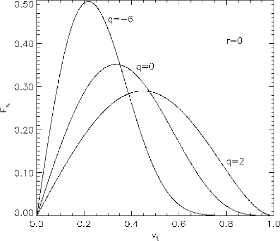
(a)
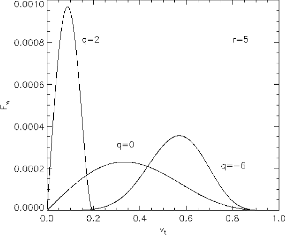
(b)
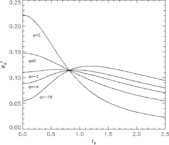
The DF (2.20) contains all the information about the Plummer sphere it represents, and by integrating it out and computing its various moments a number of useful quantities and observables can be derived. Two of them, the distribution of the transverse velocities and the projected velocity dispersion as a function of the projected radius , are particularly well suited to test Schwarzschild’s method. This is so mainly for two reasons. First, they reveal velocity information that was not constrained when the Schwarzschild equilibrium was constructed, thus enabling one to gain a feeling of the level of irregularity (lack of smoothness) present in the equilibrium. Second, because is an observable that will also be numerically estimated for the triaxial Dehnen potential, it is useful to see how robust this estimate is. These two quantities are given by the following expressions:
| (2.23) |
and
| (2.24) |
Figures 2.1 and 2.2 graphically depict Eqs. (2.23) and (2.24), respectively, for various values of . One can infer from Figure 2.1 that for a maximally radially anisotropic () system, the mean of the tangential velocity distribution decreases with increasing distance from the center. The opposite is true for a tangential () system, while in the isotropic () case the shape of the distribution remains unchanged. This complementarity property can also be seen in the projected velocity dispersion, where, at small radii, is higher in radial systems rather than in tangential systems, but the opposite is true at large radii. Another interesting observation is that all curves intersect at a single point . This is a consequence of the fact that enters linearly in both the numerator and denominator of Eq. (2.24).
There is an important question one has to address before proceeding to a meaningful comparison between analytical and numerical predictions. Are all these analytical results generic or do they reflect the peculiarities of the decomposition of into an augmented (Eq. 2.19)? If they do reflect peculiarities of the decomposition, to what extent would this harm the comparison between theory and numerical results? Unfortunately, there is no easy answer to this question. Dejonghe’s choice of the functional form for an augmented density is certainly quite special and serves mathematical convenience above all. At the same time, there is no general method that would allow one to explore the entire range of possible augmented densities that correspond to a given . Nevertheless, it may not be unreasonable to expect that at least certain qualitative conclusions and trends might remain valid over a considerable range of choices for the functional form of the augmented densities. For instance, one might expect that the complementarity property would transcend specific choices of . One might also argue that, given enough templates in the library of orbits (or, strictly speaking, given an infinity of orbital templates), Schwarzschild’s method ought to be able to select those that correspond to any feasible DF, including Dejonghe’s. However, even if it were practical to have an infinity of templates in the library of orbits, one would also have to force the optimization method to seek a particular solution, which should somehow be encoded in the cost function and the constraints of the problem (§2.8). This is not always trivial to do, especially if one is limited to, at most, quadratic cost functions with a linear set of constraints.
The remainder of this Chapter describes the process of computing numerical DFs of a Plummer sphere using Schwarzschild’s method, and then uses these numerical DFs to extract the distributions of transverse velocities and projected velocity dispersions for comparison with Dejonghe’s corresponding analytical results.
2.6 The Library of Orbits
| Shell | Shell | ||||||
|---|---|---|---|---|---|---|---|
| 1 | 0.388906 | -0.931999 | 0.271366 | 11 | 1.362183 | -0.591774 | 0.870309 |
| 2 | 0.513324 | -0.889636 | 0.355016 | 12 | 1.487087 | -0.558021 | 0.939376 |
| 3 | 0.613219 | -0.852481 | 0.420643 | 13 | 1.629227 | -0.523110 | 1.016486 |
| 4 | 0.703477 | -0.817894 | 0.478712 | 14 | 1.794980 | -0.486680 | 1.104688 |
| 5 | 0.789792 | -0.784761 | 0.533156 | 15 | 1.994166 | -0.448259 | 1.208643 |
| 6 | 0.875303 | -0.752464 | 0.586069 | 16 | 2.243022 | -0.407193 | 1.336033 |
| 7 | 0.962213 | -0.720590 | 0.638844 | 17 | 2.571058 | -0.362492 | 1.500801 |
| 8 | 1.052389 | -0.688833 | 0.692590 | 18 | 3.039622 | -0.312511 | 1.731995 |
| 9 | 1.147675 | -0.656935 | 0.748334 | 19 | 3.806974 | -0.254057 | 2.104982 |
| 10 | 1.250114 | -0.624660 | 0.807155 | 20 | 5.499692 | -0.178895 | 2.921630 |
The first step in the implementation of Schwarzschild’s method is the construction of a library of orbital templates. As explained in §2.1, the central concern in this enterprise is to ascertain that the library offers a comprehensive coverage of the phase space accessible to the DF that is going to be built. In view of the inaccuracies introduced in the coarse-graining (§2.7) and optimization (§2.8) stages, it may not matter a lot if families of orbits that do not support considerable structure in the sought-after DF are omitted or underrepresented —the deficit will be overshadowed by the numerical errors. However, if critical families of orbits are omitted, the consequence could be that the optimization problem is infeasible. In such a case, one cannot a priori know if infeasibility is due to an inadequate library or because there can exist no time-independent DF capable of supporting the imposed mass density distribution . In practice, these considerations mean that the next best thing to having an infinite sample of orbital templates would be to (i) identify the important families of orbits in the potential produced by , and (ii) include as many of them as computationally possible.
The choice of initial conditions for the Plummer sphere is relatively straightforward. It is an integrable system, and thus all orbits are regular. All that one has to do is to sample uniformly and as densely as possible any three independent integrals of the motion (e.g., ). This was implemented as follows. The Plummer sphere was partitioned into 20 equal-mass, spherical and concentric shells at radii determined from
| (2.25) |
where Eq. (2.11) was used. At each radius, the value of the energy on the isopotential surface (which, for spherical systems, coincides with the isodensity surface) was then computed from Eq. (2.13). The radii and energies are shown in Table 2.1.

Consequently, the positive octant of each isopotential surface was sampled at 40 positions, selected to be centered on segments of approximately equal area. This was done by (i) uniformly sampling the -angle variable at 7 values between 0 and , (ii) computing the surface area contained within the zones defined by each consecutive pair of constant- circles via
| (2.26) |
(iii) computing the ratio of the area covered by each zone to the area covered by the the zone (spherical triangle) closest to the axis, and (iv) partitioning each zone in equal segments. This procedure might have to be repeated a few times until the fractional part of would become small enough so that . The result can be seen in Figure 2.3.
The remaining two integrals were sampled along the line joining the center of the sphere to every selected point on the octant. The angular momentum magnitude was sampled at 5 radial points between the radius of maximum angular momentum (circular orbit) and the isopotential (zero-velocity) surface, using
| (2.27) |
where and and (purely radial or purely circular orbits are not desirable because they introduce numerical singularities which could be amplified by the numerical inversion). In order to evaluate , the circular velocity radius and the circular velocity can be found by combining the expression for centrifugal acceleration
| (2.28) |
with conservation of energy at (where )
| (2.29) |
which yields
| (2.30) |
This equation can be numerically solved for given the energy of the orbit and setting (see Table 2.1). Once is known, can be found from Eq. (2.28) and can be evaluated. The initial position then is set to , the initial tangential velocity is and the initial radial velocity is obtained from the energy.
Finally, the second component of the angular momentum is chosen by specifying how is decomposed into and , effectively defining the inclination of the orbital plane with respect to the plane. A total of 5 angles were computed for every value of via
| (2.31) |
so that and . This last step could no doubt be avoided. Indeed, all the orbits computed separately for each value of will be identical modulo a rotation. One can take advantage of the spherical symmetry and estimate the contributions of the entire continuum of orbits in from an orbit computed for a single . However, such a convenience is not available in a triaxial potential. Since the purpose of this experiment is to test Schwarzschild’s method with the ultimate goal of applying it to the triaxial Dehnen potential, no advantage of the spherical symmetry was taken in the construction of the library of orbits. In fact, this decision places the Plummer sphere at a disadvantage compared to a triaxial potential, because, as noted earlier, the Plummer orbits are delta-functions (planes) in the three-dimensional configuration space, whereas orbits in triaxial potentials are generally non-planar and, hopefully, numerically better behaved. In that sense, the Plummer sphere actually represents a “worst case” problem for Schwarzschild’s technique.
At the end of this process, a total of orbital templates are included in the library.
Once the initial conditions of the orbital templates that will make up the library are selected, the next concern is to ensure that the time-averaged configuration-space density of each template does indeed remain (nearly-)time-indepen-dent (cf. Eq. 2.3). This requirement is at least as important as the the one for comprehensive phase-space coverage. If the building blocks are not truly time independent, neither will the “equilibrium” made out of them be.
For regular orbits, such as those that populate Plummer spheres, one has to make sure that each orbit has been given enough time to uniformly cover its action torus. If the orbit is closed, or in other words the ratio of its radial to its azimuthal period is a rational number, then one would have to integrate that orbit for precisely an integer number of the least common multiplier of the two periods. However, regular orbits of nontrivial potentials are not generally closed, and chaotic orbits are aperiodic. The time required for uniform coverage of the action torus of the former, or the constant- or constant- hypersurface of the latter actually depends on the coarse-graining of the configuration space. Hence it is desirable, for the sake of numerical convenience, to devise a more general way of figuring out for how long to integrate an orbit.
Pfenniger (1984) proposed an iterative method, which does not depend on whether an orbit is regular (closed or open, low- or high-order resonant) or chaotic. The method consists of the following three steps, in a slightly different formulation from the original:
- Step 1:
-
Integrate the orbit over a number of typical crossing (or dynamical) times and compute how much time it spends in each configuration space cell (§2.7). In other words, compute the column in matrix that corresponds to orbit integrated over crossing times. Normalize so that, e.g., .
- Step 2:
-
Integrate orbit for another , thus obtaining a second column matrix , and normalize again.
- Step 3:
-
If the norm , where is a small positive number of order , then average and and repeat Step 2. Otherwise, the method has converged and the computation is terminated.
This method is guaranteed to converge (i.e., exists) for any regular orbit, though it may take several iterations depending on any high-order resonances and the level of coarse graining of the grid. Pfenniger found that the method would not always converge for chaotic orbits, even after long integrations. If, however, one computes the average of the ’s that correspond to all the chaotic orbits of a given energy, one would usually find much faster convergence rates (Kandrup and Mahon, 1994) (see also §3.5).
The importance of using time-independent building blocks cannot be overemphasized. Some workers have simply integrated orbits for a “long enough” period of time, usually comparable to a Hubble time . The implicit argument here is that if, after more than a Hubble time, an orbit enters new phase-space domains, that would have no effect for a real galaxy. However, the orbital integration time is entirely irrelevant to the age of the universe. These are actually orbital templates, in the sense that actual orbits can be sampled anywhere along them. To give a somewhat contrived example, if nature places a star near the end of a computed orbit that has been terminated just before it was about to enter uncharted territory then the model will clearly not be time-independent.
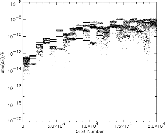
The orbits were calculated by integrating the equations of motion (2.14) using a Bulirsch-Stoer integrator (Stoer and Bulirsch, 1980, §7.2.14) (see also Press et al., 1992, §16.4). This method was chosen because of its high numerical accuracy and computational efficiency when integrating smooth functions. However, it later became apparent that using a symplectic integrator might have been a better choice, because it would preserve the Hamiltonian nature of the integration, which would arguably be useful, particularly for the chaotic orbits of the triaxial Dehnen potential. Moreover, in order to avoid interpolating between orbital points too far apart, Bulirsch-Stoer was forced to produce output every tenth of a dynamical time, which was often too short compared to the method’s own choice of integration timestep, thus losing some efficiency. Nevertheless, Bulirsch-Stoer was twice as fast as a 5th order Runge-Kutta that was also tried, and it conserved energy better than one part in for most orbits after 200 dynamical times (Figure 2.4).
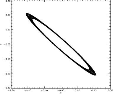
(a)
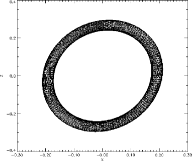
(b)
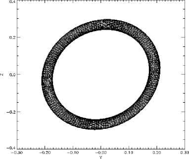
(c)
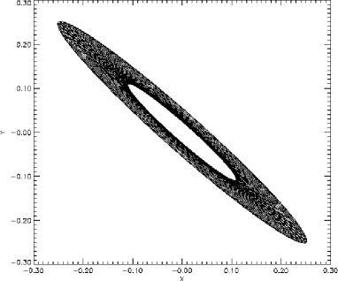
(a)
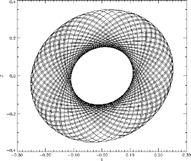
(b)
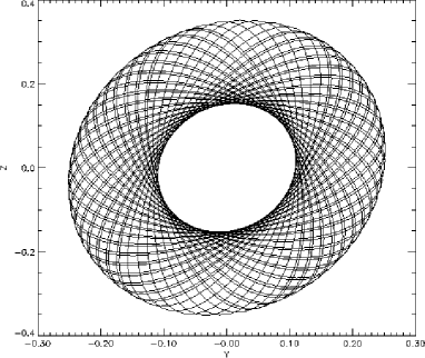
(c)
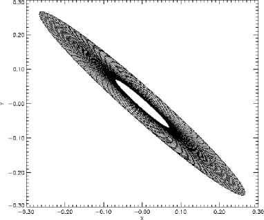
(a)
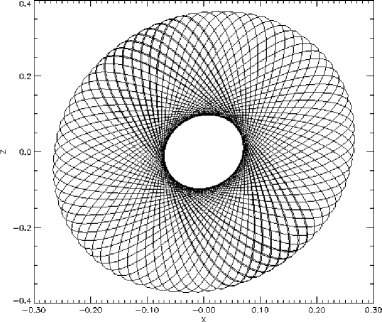
(b)
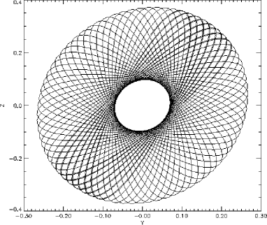
(c)
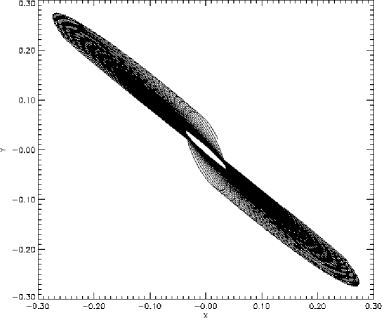
(a)
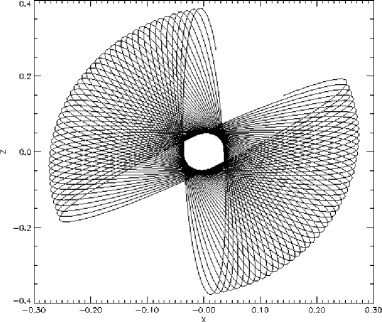
(b)
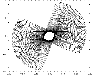
(c)
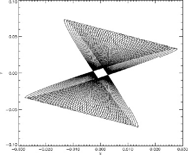
(a)
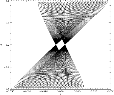
(b)
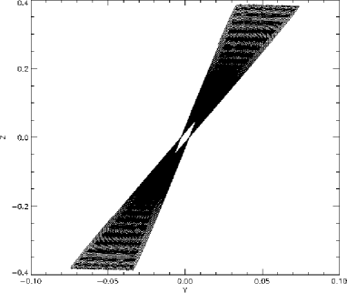
(c)
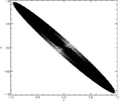
(a)
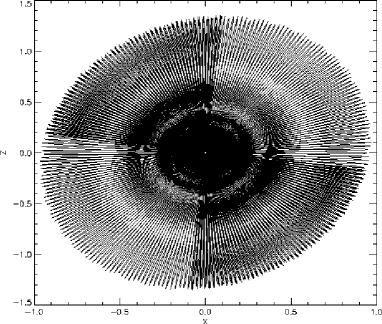
(b)
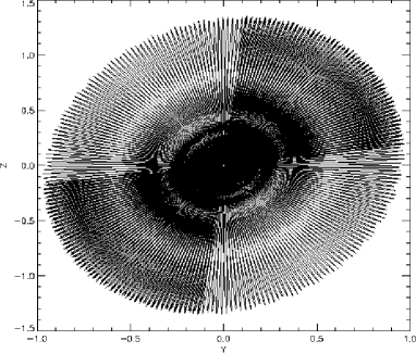
(c)
Figures LABEL:2.fig.orb0 – 2.9 depict the first five orbital templates in the library. They show the characteristic rosette shapes of integrable motion. As the angular momentum of each consecutive orbit decreases, it makes closer passages to the center. At the same time, the rate of azimuthal motion drops, so that, in 200 circular-orbit dynamical times, a highly eccentric orbit traces only part of its resonant torus (Figures 2.8 and 2.9). This effect is less pronounced in the outer parts of the system, where low-angular-momentum orbits do fill out their resonant tori. However, as can be seen from Figure 2.10, there are still considerable density contrasts between the regions that were covered only once and the regions the orbit had enough time to visit for a second time. Such differences exist for near-circular orbits as well (see, for instance, the second and fourth quadrant of Figure 2.7b) but they are less pronounced because they are spread over a larger surface area of the torus, owing to the fact that these orbits’ motion in the azimuthal direction is faster.
In spite of what was said earlier regarding integration times, the orbital templates for the present work were integrated for a fixed period of 200 dynamical times, or more precisely, 200 times the orbital period of a circular orbit of the same energy. One reason why this was done was to show how bad the problem of using building blocks that are not truly time-independent can be in the “worst-case” scenario of a Plummer sphere. More specifically, the results one gets by considering the computed orbits of low angular momentum as time-independent building blocks, when in fact they are not, will be compared (§2.9) with the results one gets by discarding the orbits with the two lowest values of angular momentum, i.e., orbits generated for and in Eq. (2.27).
However, there was also another, more practical, reason for integrating
over a fixed length of time, namely hardware limitations. An
implementation of Pfenniger’s method would require some orbits to be
integrated for very long times. Because the library of orbits is actually
stored on disk (so that velocity moments and other quantities can be
computed once a model is constructed), storing the library orbits
would require more disk space than was available for this project.
Furthermore, in the nonintegrable triaxial problem the orbits “spread
out” more and the deviation from being truly time-independent building
blocks are less severe. Nevertheless, future work (Chapter 4) will
implement a variation of Pfenniger’s method.
2.7 The Coarse-Graining of Configuration Space

The configuration space was coarse-grained using a grid similar to the one used by Merritt and Fridman (1996), which was in turn based on the grid used by Schwarzschild (1979). The radial dimension is divided by 20 concentric spherical shells, each containing of the total mass. The last shell extends to infinity and is not included in the self-consistent problem. These are the same shells on which the initial conditions were sampled (§2.6). Each shell is divided into three segments by the planes , and , as shown in Figure 2.11, and each segment is further divided into 16 facets, using a set of three planes in one direction and three in the vertical direction. For instance, the lower-left segment is divided by the 3 planes and , and similarly by the planes and . This way, a total of cells are created. Such a grid geometry has the numerical advantage that it places similar masses in each cell.
The time (Eq. 2.1) that each orbit spends inside every cell is computed with high accuracy using the following method. While the orbit remains in its current cell, time is advanced in steps of (the library output timestep). When a step of brings the orbit outside its current cell, the timestep is reduced by a factor of ten, and the process is repeated until the orbit exits the cell with the smaller timestep, at which point the step is reduced once again by a factor of ten. This way, can be found with an accuracy of . The orbit position between stored library positions is found using linear interpolation. More sophisticated interpolation schemes, such as splines, are avoided because they can and do produce spurious results, especially with irregularly shaped chaotic orbits.
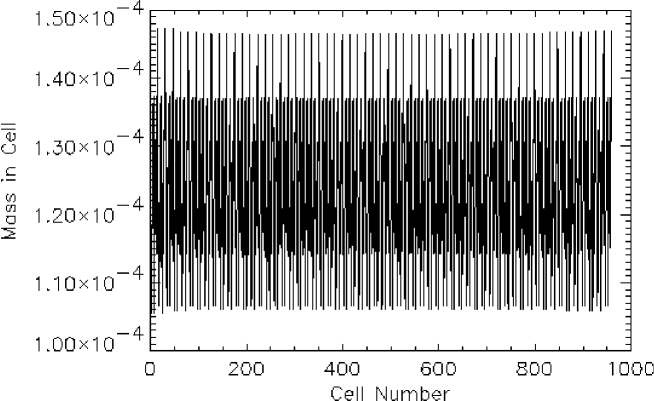
(a)
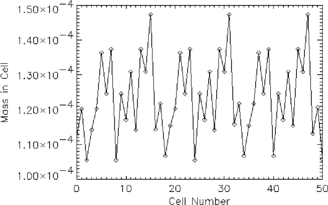
(b)
Finally, the mass that the Plummer sphere density law places inside every cell has to be computed. Given the relatively complex definition of cell boundaries, the direct analytical evaluation of
| (2.32) |
is somewhat complicated. Instead, the above integral is estimated numerically by gridding the octant with a very fine rectangular mesh of variable resolution (finer close to the center, where cells are small, and becoming coarser with increasing radius) and adding the density contributions on each grid node. Figure 2.12 shows mass variation with cell number. Masses are similar to within a factor of 1.5.
2.8 The Optimization Problem
At the heart of Schwarzschild’s method lies the constrained optimization problem that solves the system of equations [cf. Eq. (2.1)]
subject to
In general, the problem can be stated as follows:
| Minimize: | |||||
| subject to: | (2.33) | ||||
| and: |
where , the cost or objective function, is a linear function of the weights. In the astronomical literature, this problem is usually solved using a SIMPLEX-type algorithm (cf. e.g., Schwarzschild, 1979; Richstone and Tremaine, 1984; Statler, 1987), a nonnegative least squares (NNLS) algorithm (cf. e.g., Pfenniger, 1984; Zhao, 1996; Wozniak and Pfenniger, 1997; Rix et al., 1997), quadratic programming (Merritt and Fridman, 1996), nonlinear optimization (Levine and Sparke, 1994) when the cost function and/or the constraints are nonlinear, or Lucy’s method (Newton, 1983; Newton and Binney, 1984; Statler, 1987). Of these techniques, Lucy’s method is distinctly different, being a Bayesian iterative deconvolution scheme. Statler (1987) used Lucy’s method to establish the existence of a solution and then switched to linear programming to map out the boundaries of the solution space. Newton (1983) found that linear programming produced DFs with large short- and long-wavelength fluctuations whereas Lucy’s method produced smooth, rapidly converging DFs.
The present work made use of a quadratic programming (QP) algorithm, whereby the quadratic part was used solely to impose a level of smoothness to the distribution of the weights . Although Lucy’s method was not implemented or compared against QP, experimentation in the present work with the QP algorithm (which also includes linear programming (LP) as a special case) suggests that it is not necessarily intrinsically inferior to Lucy’s algorithm in terms of constructing DFs. QP/LP faithfully does what it is explicitly told to do: it precisely obeys the constraints and optimizes the cost function, and it does that fairly well. However, once it satisfies its constraints, it does not make any effort to provide a solution that would be agreeable to the astronomer (such as one that obeys some smoothness constraint) unless the astronomer identifies the extra constraints and demands that they be obeyed (by adding extra constraints and/or specifying an appropriate cost function).
This may explain some of the frustrating results that certain workers obtained using LP. By solely requiring that the Plummer density law be respected in every cell, one tacitly implies that this is all the physics that there is. But in reality, one also knows that smoothness of the DF should also be a constraint, both because noisy fluctuations are an expected numerical artifact of the ill-conditioned inversion, and because population inversions are known to be sources of instability (§2.1.1). When one enforces some level of smoothness, e.g., by minimizing the sum of the squares of the orbital weights, the solution does become considerably smoother (though perhaps still not as smooth as a Lucy solution).
For this work, it was decided that the cleanliness of the constraints mechanism associated with QP/LP is arguably preferable to the enforced smoothness of the Lucy algorithm. A maximum likelihood approach could still be fruitful, but only after all physically motivated constraints have been exhausted.
Another approach is the NNLS method, which reformulates problem (2.8) as follows:
| Minimize: | ||||
| subject to: |
where is a positive constant. Wozniak and Pfenniger (1997) argue that an advantage of NNLS over LP is that, when no exact solution exists, NNLS still converges to the nearest approximate solution, in a least-squares sense, whereas LP simply fails (one might argue that such an “approximate” solution may actually be quite far away from any physical solution, but it may still be useful as an indicator of where the problem lies). However, it is possible to avoid this problem by reformulating the LP problem as follows:
| Minimize: | |||||
| subject to: | (2.35) | ||||
| and: |
where is a positive constant. This way, the LP algorithm is always feasible, and any deviations from exact self-consistency can be found by inspecting the values of and .
In fact, as was discussed above and will be seen in the next section, if one simply solves the above LP problem, the solution can be quite noisy and unphysical, with entire ranges of orbits carrying zero weights. One can improve upon this undesirable situation by demanding, e.g., the minimization of the sum of the squares of all the orbits, in other words by solving the problem
| Minimize: | |||||
| subject to: | (2.36) | ||||
| and: |
This has now become a QP problem, defined as
| Minimize: | |||||
| subject to: | (2.37) | ||||
| and: |
where , is symmetric positive semidefinite and .
This problem is solved using BPMPD (Mészáros, 1996a, b), a state-of-the-art implementation of the primal-dual interior point algorithm for linear and convex quadratic programming problems, kindly made available by the author. The package includes highly flexible sparsity handling, fast and robust linear algebra and advanced presolve techniques. It was compared to several other SIMPLEX and Interior Point software packages in the public domain and it fared better both in terms of speed and memory requirements. A QP problem would take, depending on the sparsity of the matrix , between 60 and 150 minutes on a Pentium Pro 200 MHz-class computer with 128 Mb of RAM, running under Linux.
2.9 Nonuniqueness of the Solutions: Comparison with Analytical Results
The optimization techniques described in the previous section will now be applied to attempt to reproduce the analytical results presented by Dejonghe (1987), and in particular Figures 2.1 and 2.2 (§2.5). In order to numerically reproduce the effects of varying the anisotropy parameter , a series of four optimization runs was effected, corresponding to a minimization or a maximization of the number of low angular momentum orbits, performed using LP and QP.
It is appropriate to ask whether a better way exists to numerically
mimic variations of . The answer is most probably yes: it would be
possible to implement additional constraints in every grid cell, that
would enforce a particular anisotropy behavior. However, the aim here
again is to test Schwarzschild’s method before it is used to study the
nonuniqueness properties of the triaxial Dehnen potential. Even though one
could attempt to enforce some kind of velocity anisotropy or velocity
dispersion profile to the triaxial case, the lack of knowledge of a DF
carries the danger of demanding a velocity anisotropy or dispersion
profile that is unnatural and hence infeasible. Since the main question
for the triaxial case is whether it is possible to have two DFs with
considerably different amounts of chaos, but both supporting the same mass
distribution, it only makes sense to minimize or maximize the number of
chaotic orbits and see what effect this has to the velocity dispersions.
Therefore, it is appropriate to pose a similar problem in the Plummer case
as well, and attempt to minimize, or maximize, a particular class of
orbits.
2.9.1 Minimization of Low- Orbits
In order to minimize the number of orbits with low angular momenta, the optimization problem (2.8) is solved for the following cost function:
| (2.38) |
and the square brackets represent the integer part of the argument. This formulation makes use of the fact that the orbital templates in the library come in successive quintets of decreasing angular momentum. The above definition for places negative coefficients in front of the two highest-angular-momentum families of orbits. Since (2.8) is a minimization problem, this causes their weights to be maximized (the more they are used the lower the cost function becomes). By contrast, the orbits with the remaining three values of (lower) angular moment have positive coefficients. Their presence increases the cost function, thus making them undesirable.
Figure 2.13 shows the distribution of weights returned by the optimization software. Figure 2.13c confirms that the model is feasible, since the mass placed inside every cell agrees with the Plummer density law to within single machine precision. It is immediately apparent from Figure 2.13a that the LP algorithm uses as few orbits as it needs to create the model and discards the rest, setting their weights to essentially zero. There are 4794 orbits with weights greater than , of which only 953 have weights greater than . This number is essentially equal to 960, the number of cells in the grid. Indeed, linear programming, by construction, finds only as many nonzeros as the number of constraints (cells).
Obviously, this is an undesirable and unphysical numerical artifact. To
ameliorate the situation, one can solve the QP problem (2.8).
The results are shown in Figure 2.14. There are now 4492
orbits with , 4031 of which have , a
significant improvement. Nevertheless, it is obvious that there is no
reason why more orbits could not be used. Using an alternative quadratic
term and/or increasing the number of cells/constraints could perhaps
involve more orbits in the DF.
2.9.2 Maximization of Low- Orbits
In a way similar to the one used in the previous paragraph, the cost function is now set to be
| (2.39) |
The coefficients are now positive for the orbits with the three highest angular momenta, and negative for the remaining two. The results are shown in Figure 2.15 for the LP problem and in Figure 2.16 for the QP problem. One can see that, even though self-consistency is satisfied, at least to within the level of coarse-graining of the model, the DF itself is “hollow”: the orbits sampled in the six innermost shells are left almost entirely unpopulated, both in the LP and the QP models. Such a model seems unphysical and may quite likely be unstable.
Most probably, this result reflects the problematic low-angular-momentum
orbital templates of the library, which are not truly time-independent. As
was pointed out in §2.6, low- orbits close to the center
have entire segments of their resonant tori unoccupied because they were
not integrated for long enough. This effect is less severe with the
low- orbits in the outer parts of the system, which do cover
their entire resonant tori albeit not uniformly. The optimization
algorithm then rejects the inner low- orbits because they violate the
spherical symmetry of the system, though its still manages to use the
outer low- orbits. However, if the resolution of the grid were to
become finer or the number of constraints otherwise increased, the problem
would most probably become infeasible.
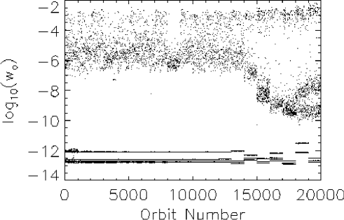
(a)
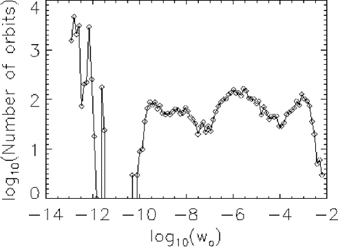
(b)
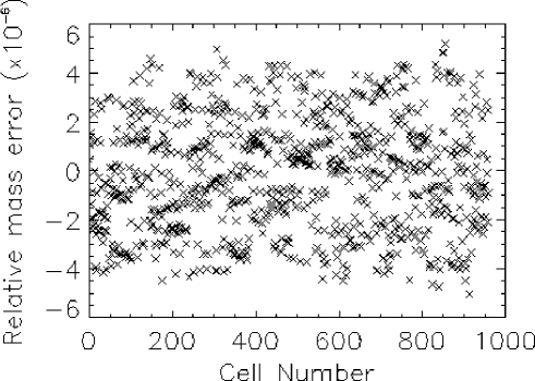
(c)
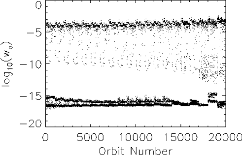
(a)
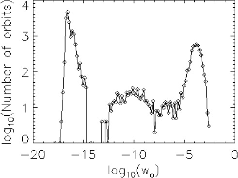
(b)
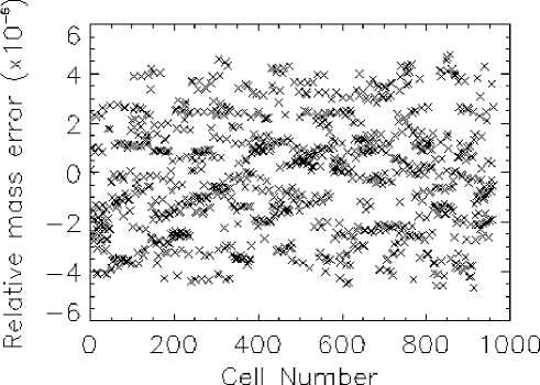
(c)
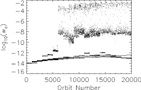
(a)
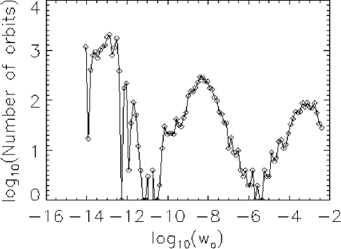
(b)
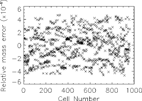
(c)
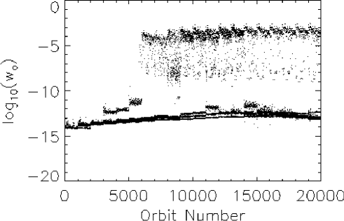
(a)
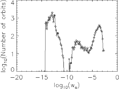
(b)
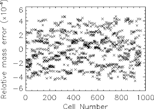
(c)
2.9.3 Transverse Velocity Distributions and Projected Velocity Dispersions
The distribution of transverse velocities inside a given spherical shell was computed by taking into account the portions of all orbits entering that shell. To this effect, the positions and velocities of orbits were sampled at ten times the library sampling rate, using linear interpolation to avoid smoothing side-effects of more sophisticated methods such as splines, and were then converted to spherical coordinates.
The results are shown in Figure 2.17 for the LP DFs and in Figure 2.18 for the QP DFs. The transverse velocity distributions constructed from DFs that maximized the number of transverse orbits (solid lines) clearly follow the trend exhibited by the analytic models (Figure 2.1, ): the mean of their distributions systematically increases with radius while, at the same time, the area under the distribution (which is proportional to the local density) decreases. The numerical distributions appear narrower than the analytic ones, but this can be explained at least in part from the fact that the numerical distributions were computed over the range of radii that corresponds to the width of every shell, whereas the analytical distributions were found for a single value of the radial coordinate: In the analytical case, the normalization of the abscissa is such that the maximum (escape) velocity for that radius is equal to 1. However, for the numerical distributions, the escape velocity was computed for the inner shell radius, where it is faster than for the outer radius, and hence the shape of the distribution appears more “compressed” in the horizontal direction.
One can also see that the numerical distributions do a rather good job, at least for small radii, in imitating the bell-like shape of the analytical distributions. However, it is also obvious that they contain lots of structure. In particular, there is clear evidence of a bimodal distribution for most radii, and even hints for a trimodal distribution at . It was argued in §2.5 that Dejonghe’s choice of decomposing is certainly not unique, and so one might be tempted to interpret the bimodal distributions at face value, as being suggestive of a DF different from Eq. (2.20). Nevertheless, such an interpretation is most probably incorrect. Although the presence of the bimodal distribution in the numerical DF is beyond doubt, it is most probably related to the small number of values (5) for which the angular momentum was sampled. There were simply not enough orbits with a continuum of angular momenta to make “rough edges” such as these disappear.
The agreement between analytics and numerics is somewhat worse for the transverse velocity distributions generated from the numerical DFs that maximize the number of radial orbits (dashed lines). Here the analytical results indicate that, as one moves away from the center, the mean of the velocity distribution should shift to lower values while at the same time the peak value should grow with respect to the solid-line peak. Indeed, if one ignores the peak on the lowest-velocity bin, there is a clear trend that does precisely what the analytical work suggests, modulo bimodal features and rough edges similar to the ones encountered in the previous case. However, instead of the distribution being “absorbed” smoothly into the low-velocity bin at large radii, it seemingly disappears quite abruptly near . From that point on, there is virtually no high-transverse-velocity component in the system. In any case, however, it is not reasonable to expect that this velocity distribution is legitimate, since the DF itself, which contains hardly any orbits in the low-energy shells, is unphysical.
Overall, it seems fair to say that the the transverse velocity distributions, drawn from both numerical DFs, look quite reasonable, especially in view of the caveats at the beginning of this Chapter. Furthermore, for those aspects of the distributions that look less believable, there is usually a readily identifiable numerical reason for why this is so. Interestingly, there are very few differences between the velocity distributions computed from the LP and the QP problem.

![[Uncaptioned image]](/html/astro-ph/9902089/assets/x40.png)
Figure 2.17–continued
![[Uncaptioned image]](/html/astro-ph/9902089/assets/x41.png)
Figure 2.17–continued

![[Uncaptioned image]](/html/astro-ph/9902089/assets/x43.png)
Figure 2.18–continued
![[Uncaptioned image]](/html/astro-ph/9902089/assets/x44.png)
Figure 2.18–continued
Finally, the projected velocity dispersions were computed on the three principal planes by projecting the velocities into each plane, dividing the plane into 20 concentric annuli, and then averaging over the angular dependence with each annulus. The mean and the variance of the projected (perpendicular to the principal plane) velocities inside every annulus were obtained from the usual relations
| (2.40) |
where represents the portions of the projected velocity time series of any and all orbits entering a given annulus. Again, the positions and velocities of orbits were sampled at ten times the library sampling rate, using linear interpolation. The velocity dispersions were then obtained from
| (2.41) |
The results are shown in Figure 2.19. The graphs for all three principal planes look indistinguishable (as a result of the symmetry of the system but also of the symmetrical way in which the orbits were selected). Interestingly, the graphs for the DFs derived from LP and QP also look identical (though upon inspection of the numbers they do differ at the fraction-of-a-percent level). For these reasons only the plot of the velocity dispersion obtained from the LP DF on the plane is shown. Comparison with Figure 2.2 is very good.

Chapter 3 SELF-CONSISTENT MODELS OF TRIAXIAL DEHNEN ELLIPSOIDS
This Chapter describes the use of Schwarzschild’s numerical method for the construction of self-consistent triaxial Dehnen ellipsoids. The principal aim is to test the degeneracy of the solutions in terms of the range of possible variations in the relative abundances of chaotic and regular orbits populating the models.
3.1 Motivation
The role of chaos in the structure and dynamics of galaxies is an issue still debated in the galactic community. While it is known that integrable potentials form a set of measure zero in the space of potentials, there is no a priori reason to exclude the possibility, however seemingly far-fetched, that the mechanics of galaxy formation somehow favor (or lead to) mass density distributions that generate integrable potentials, e.g., via some sort of feedback mechanism related to “violent relaxation.”
A more fruitful way to approach the question of the role of chaos in galaxies would arguably be to construct self-consistent models of galaxies, as opposed to studying fixed potentials, for which one often cannot know in advance whether they can be self-consistently supported via Poisson’s law. There are two known ways to construct self-consistent models numerically: Schwarzschild’s method (or variants thereof, aimed at deconvolving phase-space DFs from observationally accessible quantities) and -body simulations, which are by definition self-consistent. Either one is harder to implement and interpret than studies of fixed “toy” potentials (although, of course, such studies are still necessary as precursors to the construction of a quality library of orbital templates for use with Schwarzschild’s method – see the discussion in the previous Chapter).
Unfortunately, neither Schwarzschild’s technique nor -body simulations can offer an unequivocal answer to the initial question. Even if one dismisses, for the moment, the numerical and conceptual problems associated with Schwarzschild’s method, one cannot ignore the fact that it is not possible to know whether the form of the mass density distribution that is being used for the construction of the model actually corresponds to something that exists in nature (just because it is self-consistent does not necessarily mean it exists in nature!) This is so because one cannot infer the three-dimensional from two-dimensional photometric observations (even assuming that the mass-to-light ratio is known) unless some assumption is made about the three-dimensional shape of the system. However, making a realistic assumption may not be trivial, given the wealth of structural detail that even elliptical galaxies often reveal upon closer inspection (isophotal twists, boxiness, diskiness, varying ellipticities with radius, embedded disks or other decoupled components, etc). -body simulations also suffer from the same problem, which is further exacerbated by the difficulty of defining and understanding chaos in -body simulations and how it relates to chaos in the collisionless Boltzmann equation111Strictly speaking, there are strong indications, both theoretical (Kandrup, 1990b) and numerical (Miller, 1964; Kandrup and Smith, 1991; Goodman et al., 1993; Kandrup et al., 1994) that, at least for , all orbits in the generic -body problem are chaotic..
Nevertheless, in the absence of any known mechanism that would force galactic potentials to become integrable, it seems legitimate to study the effects of chaos on the structure and dynamics of galaxies. A desirable by-product of such studies could be the identification of observable effects that would be characteristic signatures of the presence of chaos in galaxies. Within this framework, a study of self-consistent chaos is a major step forward from the study of chaos in fixed potentials.
Shortly after Schwarzschild (1979) introduced his method for constructing numerical equilibria, Merritt (1980) realized that the time spent by some orbits in the grid cells was different when they were integrated on a different computer. Today this would be recognized as a telltale sign of chaos, manifesting the fact that chaotic orbits exhibit an exponential sensitivity to small changes of initial conditions, which can happen when, e.g., integration roundoff errors on different computers are different. This was an early indication of the role of chaos in self-consistent models. More recently, Kaufmann (1993) and Kaufmann and Contopoulos (1996) discovered that in order to create self-consistent models of certain barred spiral galaxies, chaotic orbits are required to fill the chaotic region near corotation, where resonance overlap destroys regular motion.
Merritt and Fridman (1996) presented what may be the strongest evidence yet that chaos is required to construct self-consistent models of realistic elliptical galaxies. They were motivated by recent Hubble Space Telescope observations showing that most elliptical galaxies have central density cusps , rather than extended cores, and also by theoretical and numerical work suggesting that a central cusp or mass concentration can induce chaos in a triaxial galaxy by destroying the integrability of centrophilic box orbits (see §1.4 for more details). They used Schwarzschild’s method to construct self-consistent models of two triaxial ellipticals, one with a “weak cusp” and one a “strong cusp,” corresponding to and , respectively. They found that stochastic orbits contributed, respectively, 45% and 60% of the total mass of the system. However, these models came with a caveat, about which a few things should be said.
The construction of self-consistent models of nonintegrable systems requires a generalization of Jean’s theorem to include invariant distributions of chaotic orbits as valid time-independent building blocks (Kandrup, 1998). For a potential that obeys only one classical integral, namely the energy, the generation of the library of orbital templates has to proceed in two steps. First, the regular orbits have to be sampled as densely as possible and integrated for long enough until they populate uniformly their invariant tori, in the spirit of the discussion in §2.6. Secondly, one or more chaotic orbits have to be integrated long enough until they uniformly populate the chaotic segments of the constant-energy hypersurface. If one waits for long enough, one single initial condition sampled anywhere in the chaotic region will eventually (at the limit) pass arbitrarily close to every point in the chaotic regions of the hypersurface. In this sense, the chaotic “sea” that surrounds the islands of regularity in a nonintegrable system is filled by one single orbit. In practice, however, it is usually more efficient to integrate several chaotic orbits, sampled at different locations, and mix them (time-average their contributions to the invariant measure). The reason why this is usually a better approach is because chaotic regions in three-dimensional systems are interconnected via the Arnold web, which can inhibit phase-space transport between chaotic subdomains for very long times. If, however, more than one orbit is integrated, chances are they will start in different chaotic subdomains. The expectation then is that, even if none of them is integrated long enough to escape its own subdomain, the time-averaged distribution will be a better approximation to the invariant measure than a single orbit integrated for as long as all them together.
There is some indirect evidence in support of this conjecture from short-time Lyapunov exponent work. For example, in their analysis of orbits in a truncated Toda potential, Kandrup and Mahon (1994) found that computing short-time Lyapunov exponents for different initial conditions, each integrated for a time and then averaging up, gave a better approximation to the true Lyapunov exponent than integrating a single initial condition for a much larger time .
Merritt and Fridman found that, when they insisted that their models be constructed involving only fully mixed chaotic building blocks, no self-consistent equilibria could be found. Instead, self-consistent models could only be constructed if substantial portions of the chaotic orbits were “unmixed.” For the weak-cusp case, only the innermost six shells could be mixed; for the strong-cusp case, only the innermost two.
In this Chapter, the same potential-density model used by Merritt and Fridman (1996) is re-examined in an attempt to independently test their results. There are four main differences between the present implementation and the one by Merritt and Fridman. First, a larger (by a factor of three) library of orbits was used (20000 orbits instead of 6840); second, the library sampling was slightly different; third, the orbits were integrated for twice as long (200, instead of 100, dynamical times); fourth, chaotic orbits were distinguished from regular orbits using a somewhat different technique. A different optimization algorithm was also used, but other than improved efficiency and robustness, this difference is not expected to make any substantial difference. The question of nonuniqueness/degeneracy was also addressed by searching for models which both maximize and minimize the number of chaotic orbits.
3.2 Density, Potential and Equations of Motion
The mass density distribution that will be used is a triaxial generalization of a class of spherical models studied by Dehnen (1993):
| (3.1) |
where
| (3.2) |
and is the total mass. Mass is stratified on concentric ellipsoids with axis ratios . The parameter determines the slope of the central density cusp. For the model has a finite-density core; for the central density is infinite. In the present work, the value will be used, which corresponds to the weak-cusp model in Merritt and Fridman (1996).
The potential generated by this mass distribution for is
| (3.3) |
where
| (3.4) |
Finally, the accelerations are given by
| (3.5) |
where
| (3.6) |
and the constants are
The fact that the force depends on a nonanalytical integral makes the orbit calculations very time consuming. It should also be noted here that the two-dimensional projection of this mass distribution produces isophotal ellipses that are concentric, twisted, and have constant ellipticities. However, they do not exhibit any diskiness or boxiness. Somewhat ironically, it would be less computationally expensive to use a potential that does reproduce these features, but in the interest of comparison with Merritt and Fridman, the same form for the potential is retained for this work. However, it should be kept in mind that this potential departs from axisymmetry only insomuch as to violate the symmetry that conserves angular momentum.
3.3 The Library of Orbits
In order to generate initial conditions for the library of orbits, the mass distribution is divided into 21 shells of equal mass using 20 isodensity surfaces. The value of the energy at the isopotential surface tangent to each isodensity ellipsoid along the semi-major axis is then computed.
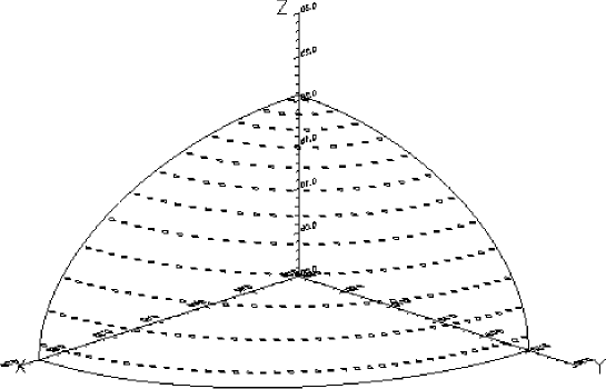
(a)
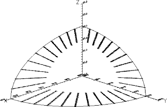
(b)
Following Schwarzschild (1993) and Merritt and Fridman (1996), the initial conditions are sampled from two separate domains, in an attempt to maximize phase-space coverage. The stationary starting space (Figure 3.1a) is comprised of orbits with zero initial velocities and initial positions sampled on the positive octant of each one of the 20 isopotential surfaces. This was done in a fashion similar to the Plummer sphere (§2.6), in other words so that each initial condition is centered on approximately equal-area segments. The two main differences from the Plummer case are that (i) the isopotential and isodensity surfaces are not identical any more, so that one has to seek numerically the intersection between the isopotential surface (given by Eq. (3.3) in a nonclosed form) and the straight line joining the center and a point on the isodensity surface; and (ii) the area of a segment of an ellipsoid is not available in a closed form, so that it, too, has to be computed numerically from the second part of Eq. (2.26), where now corresponds to , given by Eq. (3.2). A total of 250 orbits are sampled on every isopotential surface. Most are centrophilic box orbits (Figure 3.3), and most are chaotic, presumably due to their close passages to the center (Gerhard and Binney, 1985).
The principal planes starting space corresponds to orbits started on the and planes. A total of 250 orbits were sampled on each plane, covering an annulus with an inner radius equal to the minimum of the amplitudes of the 1:1 periodic orbits at that energy and on that plane, and with an outer radius defined by the curve where the potential is equal to the energy of the orbit (Figure 3.1b). The two velocity components parallel to the principal plane were set to zero, and the perpendicular component was computed from the energy with a positive sign. Most of the orbits from the principal planes space are centrophobic tube orbits (Figure 3.4), and most are regular.
A total of principal planes initial conditions were sampled at each energy level, which, together with the initial conditions of the stationary starting space, defines 1000 orbits per energy level for a grand total of 20000 orbits. Each orbit was integrated for a time equal to 200 crossing times of the 1:1 periodic orbits of that energy. This represents almost 3 times as many orbits integrated for twice as long as in Merritt and Fridman (1996). Furthermore, these authors only used principal plane initial conditions from the plane, whereas for this work, orbits from all three planes were included, thus respecting better the symmetries of the system.
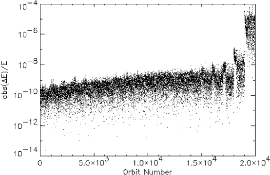
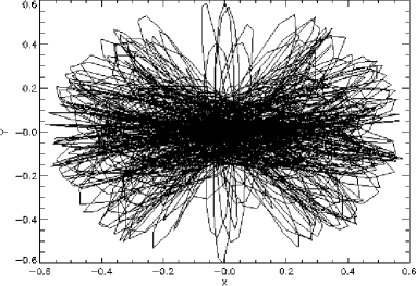
(a)
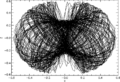
(b)
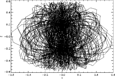
(c)
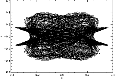
(a)
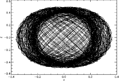
(b)
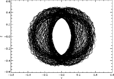
(c)
The same Bulirsch-Stoer method used for the integration of the Plummer sphere orbits was also used for the triaxial Dehnen potential. The integral in the acceleration equation (3.5) was computed using a 32nd-order Gauss-Legendre quadrature scheme. Energy conservation was better than 1 part in for most but the highest-energy orbits (Figure 3.2). Poor energy conservation for these high-energy orbits had to do with the much longer dynamical timescales in the outer parts of the system, which led to longer real-time integrations, as well as to the near-zero energies of the outermost orbits, which enter the denominator of the relative energy error calculation. It would be possible to improve energy conservation by using a higher order quadrature scheme, but this was not deemed necessary for mainly two reasons: first, improved orbital positions would not make a big difference at the level of coarse-graining of the model; second, random numerical integration errors act, in some sense, as noise, facilitating phase-space transport of confined chaotic orbits, thus making these orbits more appropriate time-independent building blocks.
Because regular and chaotic orbits need to be treated differently when solving the optimization problem, it is important to be able to distinguish between regular and chaotic orbits. For this reason, chaotic orbits have to be identified first. This was done by calculating the largest Lyapunov characteristic number associated with every orbit (§1.3.2). The numerical technique for evaluating was essentially a short-time implementation of Eq. (1.24): for every initial condition in the library, a “companion” initial condition was created by perturbing the coordinate by . Both initial conditions were actually evolved into the future, and the companion orbit’s phase-space distance from the primary orbit was renormalized to every dynamical time.
3.4 The Coarse-Graining of Configuration Space

The configuration-space grid used to solve the optimization problem is similar to the one used for the Plummer sphere models. The only difference is that the three segments are now defined by the planes and , to take into account the differing axis ratios of the ellipsoid (Figure 3.5).
3.5 The Optimization Problem
As explained in §3.1, the presence of chaotic orbits necessitates an alternative approach to computing DFs. Specifically, the chaotic orbits at every energy level have to be time-averaged and treated as one single orbit, if the ensuing model is to represent a true equilibrium. One good way to do that is using Pfenniger’s technique, outlined in §2.6. However, again in the interest of a comparison with results obtained by Merritt and Fridman (1996), their approach was used: once the library of orbital templates was computed, the chaotic orbits were identified (see next paragraph), and their contributions to each grid cell were added together and averaged out.
The identification of chaotic orbits was done differently from Merritt and Fridman. For every energy level, the distribution of the short-time Lyapunov exponents for the entire ensemble of 1000 orbits was plotted (Figure 3.7). The plots exhibit a bimodal distribution: the low- component corresponds to orbits which are either regular or confined chaotic, temporarily trapped near islands of regularity. The high- orbits correspond to unconfined chaotic orbits, populating the stochastic sea. An educated guess was made as to the value of a critical above which an orbit was classified as chaotic. This classification scheme has the advantage that it relies on ensembles of orbits, which make it easier to (i) identify how high can be before an orbit has to be classified as chaotic (a problem arising from the fact that only a short-time, , Lyapunov exponent and not the true limit is actually computed), and (ii) determine whether there is a significant component of confined chaotic orbits in the library (evidenced by a bimodal shape in the distribution of high- orbits), which would almost certainly lead to secular evolution. For each one of the 20 energy levels, the occupation times of all chaotic orbits were averaged up and were presented to the optimization software as a single orbit.
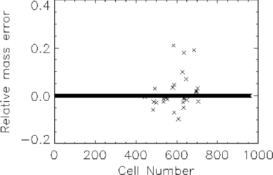

![[Uncaptioned image]](/html/astro-ph/9902089/assets/x58.png)
Figure 3.7–continued
![[Uncaptioned image]](/html/astro-ph/9902089/assets/x59.png)
Figure 3.7–continued
![[Uncaptioned image]](/html/astro-ph/9902089/assets/x60.png)
Figure 3.7–continued
The first question to ask is whether it is possible to have a self-consistent model where the chaotic orbits at all 20 energy levels are fully mixed, in the way described above. The answer is no. As shown in Figure 3.6, if one enforces mixing up to, and including, shell 14, the deviations from self-consistency in several cells become high, and the situation only gets worse as one increases the number of fully mixed shells. It is only possible to fully mix up to 13 shells before the model becomes infeasible.
The numerical DFs computed for the fully-mixed lower 13 shells included four cases: One where the number of chaotic orbits was minimized (both using LP and QP) and one where it was maximized (again, using LP and QP). In the former case, in Eq. (2.8) was given by
| (3.7) |
whereas in the latter by
| (3.8) |
where is a coefficient and “reg” and “ch” correspond to sums over regular and chaotic orbits, respectively.
The results are shown for all orbits in Figures 3.8 – 3.11, and for the chaotic orbits only in Figure 3.12. The differences between the LP and QP approach are marginal. However, there is a significant difference between the results from the cost function that minimized the number of chaotic orbits and the cost function that maximized the number of chaotic orbits. Specifically, the sum of the weights of the chaotic orbits in the first case is , compared to in the second case. Therefore, there is some freedom in the number of chaotic orbits that can populate the system. The maximum-chaos estimate places about 8% of the mass of the system in chaotic orbits, compared to 45% in Merritt and Fridman (1996). This discrepancy may be due to (i) differences in the classification of confined chaotic orbits as regular or chaotic, or (ii) the fact that the present work samples all three principal planes, instead of only the plane, thus increasing the number of mostly regular loop orbits.

(a)

(b)
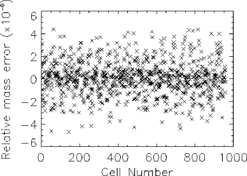
(c)
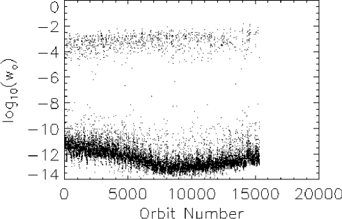
(a)
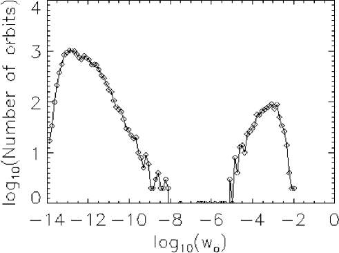
(b)

(c)
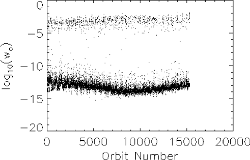
(a)
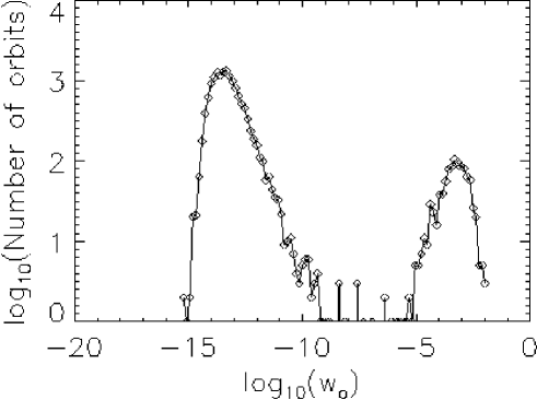
(b)
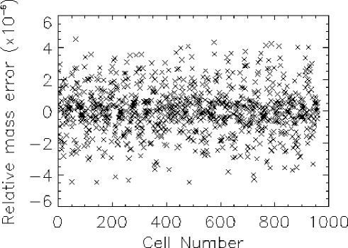
(c)
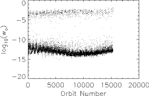
(a)
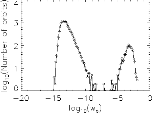
(b)
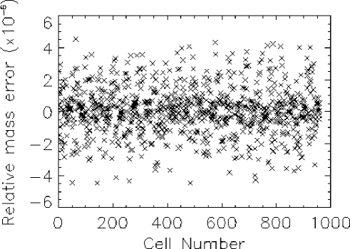
(c)
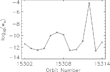
(a)

(b)
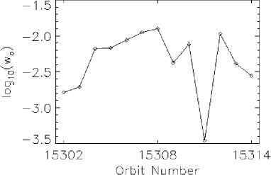
(c)
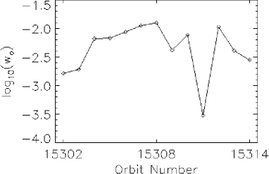
(b)
Chapter 4 CONCLUSIONS
This dissertation had two main goals. The first was to understand some of the subtleties involved in applying Schwarzschild’s method for the construction of numerical solutions (distribution functions) of the collisionless Boltzmann equation. This was effected by applying the method to a simplified problem, namely the construction of a self-consistent Plummer sphere, for which analytical solutions are known and can be used to judge the quality of the numerical solutions obtained via Schwarzschild’s method. Of particular interest was an investigation of the ability of the numerical method to reproduce at least some of the degeneracy of the solutions that is known to be there from analytical work.
The second aim was to use the expertise gained from the test problem to construct a numerical distribution function of a triaxial galaxy with a central cusp, where chaos is expected to play an important role and no known analytical solutions exist. The objectives here were (i) to compare the results from this study with results reported by Merritt and Fridman (1996) who constructed models of the same potential but in a slightly different way, and (ii) to explore the degeneracy of the solutions, in particular whether it is possible to have two alternative distribution functions, both corresponding to the same mass density distribution, but containing significantly different numbers of chaotic orbits.
The principal moral derived from the extensive use of Schwarzschild’s method in this work is that the importance of a good library of orbital templates cannot be overemphasized. The initial conditions have to be selected carefully so as to provide as comprehensive a coverage of phase space as possible. This usually means that one has to have a good understanding of the orbital structure of the system to be modeled. Failure to include enough orbits, or an injudicious choice of initial conditions that would miss important families of orbits or violate the symmetries of the system, could lead to unphysical results: one could end up with a solution that does not really exist or miss solutions that do exist. The fact that the inversion problem lying at the heart of Schwarzschild’s method is ill-conditioned only exacerbates the situation.
The principal physical conclusion is that it seems possible to achieve self-consistency for the , weak-cusp triaxial Dehnen model, at least in the innermost 13 shells, corresponding to the innermost 65% of the mass of the system. Furthermore, this could be done allowing for substantial variations in the measure of strongly chaotic orbits. It is not clear why self-consistency cannot be attained in the outer regions. One obvious possibility is that the time-averaged distribution of the outer chaotic orbits does not accurately sample the invariant measure. The rate at which orbital ensembles approach the invariant measure can vary substantially with energy and choice of potential. Similar sampling problems with the Plummer sphere models may have been the cause of observed irregularities in the tangential velocity distributions. However, these irregularities may simply reflect the fact that only five values of angular momentum were considered for each shell. This latter possibility will be checked by repeating the above calculations allowing for more values of angular momentum. Furthermore, pinning down the exact number of chaotic orbits in the triaxial Dehnen model is not trivial because of the difficulty in distinguishing between regular and confined chaotic orbits. Neither Merritt and Fridman (1996) nor this work claim to have completely solved this problem.
One obvious step in this direction would be to repeat the integration of all library orbits for considerably longer times, which would allow some confined chaotic orbits to become unconfined, thus enabling one to better distinguish between regular and chaotic orbits. Once the chaotic orbits of the ensemble have been identified, they can be integrated for very long times to yield a better approximation to the invariant measure.
Being able to distinguish properly between regular and chaotic orbits is crucial if one is to construct a truly self-consistent model. The true invariant measure of chaotic orbits at any given energy will in general contain both strongly chaotic contributions and much weaker contributions, the latter corresponding to orbits confined near regular islands. It follows that a proper “mixing” of the chaotic orbits necessarily involves combining confined and strongly chaotic orbits with the proper relative weight. Failure to do so means that one will likely construct an approximation to a near-equilibrium, characterized by near-invariant chaotic distributions, rather than to a true invariant distribution (Pfenniger, 1986; Habib et al., 1997).
Merritt and Fridman (1996) present the argument that mixing the chaotic orbits in the outer regions, where dynamical times are long, may not be required for the system to be (nearly) time-independent over a Hubble time. However, such an expectation may not be realistic, for at least three reasons. First, the orbits in the library actually represent orbital templates and their time independence has to be guaranteed irrespective of the length of a Hubble time (see discussion on page 2.3). Second, small irregularities associated with the graininess of the system (e.g., due to close encounters) can dramatically accelerate phase-space transport (e.g., Arnold web penetration) in less than a Hubble time (Pfenniger, 1986; Habib et al., 1997). Third, galaxies had to form and evolve to their present configurations. It may be unrealistic to expect that during their more violent past, galaxies were able to keep chaotic subdomains of their phase space unmixed. One might still argue that after a galaxy settles to a more relaxed state, phase-space diffusion could fill chaotic regions that are relatively isolated from each other via the Arnold web. However, such an argument implies a slow evolution with time that would alter the mass distribution and violate the initial assumption of self-consistency.
Another important extension of this work involves considering other values of , e.g., and . Such work would provide insights into the question of whether the nonexistence of self-consistent solutions really reflects the strength of the cusp. This is not completely obvious, since self-consistency breaks at large radii, where one might expect that the effects of the cusp would be especially small. Conventional wisdom suggests that there should be no problem constructing self-consistent models for the coreless case (), but this has not been shown.
The other obvious question is whether these models are stable, so that they can represent realistic configurations. This can and will be studied by generating -body realizations of the Schwarzschild models and evolving them into the future. Work on this has already begun in collaboration with E. Athanassoula of the Observatoire de Marseille using their GRAPE-3 and GRAPE-4 facilities. GRAPE (GRAvity PipE) is a massively parallel special-purpose computer for -body simulations of gravitational systems (Makino et al., 1997). The particular configuration in Marseille can reach a sustained speed of about 28 GFLOPS and can currently handle up to particles (this number is only limited by the host computer’s physical memory). The system uses a tree code, specially adapted for GRAPE’s architecture.
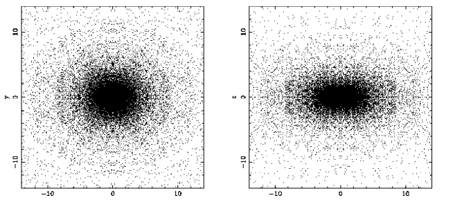
(a)
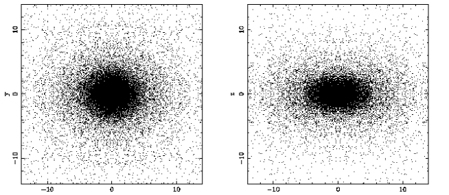
(b)
The triaxial Dehnen DFs were sampled in the following way: if the weight of a particular orbit, normalized such that , was greater than a random number in the interval [0,1], then an -body particle was generated, with the position and velocity of a random point along that orbit’s path, as sampled from the library of orbital templates. This process was repeated until the intended number of -body particles was reached. In order to help reduce large-scale fluctuations in the potential, induced by the random sampling process, the initial conditions were only sampled in the positive octant, and seven more symmetrical initial conditions were created in the remaining octants. Such measures are crucial for stability studies (Sellwood and Athanassoula, 1986).
A small number of trial -body realizations of Schwarzschild equilibria using particles have already been performed with the aim of checking whether the -body system is led to catastrophic collapse or other obvious dynamical instability. Preliminary results (Figure 4.1) suggest the system does not exhibit catastrophic changes within several inner-region dynamical times. However, there are indications that the axial ratio in the inner region of the model slowly increased from the initial value of , suggesting that the system is becoming more nearly axisymmetric. Nevertheless, at the present time it is not clear whether this effect is real or just a numerical artifact.
References
- Arnold (1989) Arnold, V. I. Mathematical Methods of Classical Mechanics. Springer-Verlag, New York, 2nd edition, 1989.
- Athanassoula (1990) Athanassoula, E. Ann. N. Y. Acad. Sci., 596:181, 1990.
- Barnes and Hernquist (1996) Barnes, J. E. and Hernquist, L. ApJ, 471:115, 1996.
- Bender et al. (1988) Bender, R., Döbereiner, S., and Möllenhoff, C. A&AS, 74:385, 1988.
- Bertola and Capaccioli (1975) Bertola, F. and Capaccioli, M. ApJ, 200:439, 1975.
- Binney (1978) Binney, J. Comments on Astrophysics, 8:27, 1978.
- Binney and Mamon (1982) Binney, J. and Mamon, G. A. MNRAS, 200:361, 1982.
- Binney and Tremaine (1987) Binney, J. and Tremaine, S. Galactic Dynamics. Princeton University Press, Princeton, New Jersey, 1987.
- Bregman et al. (1992) Bregman, J. N., Hogg, D. E., and Roberts, M. S. ApJ, 387:484, 1992.
- Carrillo et al. (1996) Carrillo, J.A., Soler, J., and Vazquez, J.L. MNRAS, 141:99, 1996.
- Carter (1978) Carter, D. MNRAS, 182:797, 1978.
- Chandrasekhar (1943a) Chandrasekhar, S. Rev. Mod. Phys., 15:1, 1943a.
- Chandrasekhar (1943b) Chandrasekhar, S. Principles of Stellar Dynamics. Chicago University Press, Chicago, 1943b.
- Channell (1995) Channell, P. S. Ann. NY Acad. Sci., 751:152, 1995.
- Cheng and Knorr (1976) Cheng, C. Z. and Knorr, G. J. Comp. Physics, 22:330, 1976.
- Contopoulos (1956) Contopoulos, G. Zeitschrift für Astrophysik, 39:126, 1956.
- Contopoulos and Grosbøl (1986) Contopoulos, G. and Grosbøl, P. A&A, 155:11, 1986.
- Contopoulos and Grosbøl (1988) Contopoulos, G. and Grosbøl, P. A&A, 197:83, 1988.
- Crane et al. (1993) Crane, P., Stiavelli, M., King, I. R., Deharveng, J. M., Albrecht, R., Barbieri, C., Blades, J. C., Boksenberg, A., Disney, M. J., Jakobsen, P., Kamperman, T. M., Machetto, F., Mackay, C. D., Paresce, F., Weigelt, G., Baxter, D., Greenfield, P., Jedrzejewski, R., Nota, A., and Sparks, W. B. AJ, 106:1371, 1993.
- Davidson (1990) Davidson, R. C. Physics of Nonneutral Plasmas. Addison-Wesley, Redwood City, California, 1990.
- Dehnen (1993) Dehnen, W. MNRAS, 265:250, 1993.
- Dejonghe (1986) Dejonghe, H. Phys. Reports, 133:217, 1986.
- Dejonghe (1987) Dejonghe, H. MNRAS, 224:13, 1987.
- Dubinsky (1994) Dubinsky, J. ApJ, 431:617, 1994.
- Eddington (1916) Eddington, A. S. MNRAS, 76:572, 1916.
- Evans (1951) Evans, D. S. MNRAS, 111:526, 1951.
- Fabbiano (1989) Fabbiano, G. Ann. Rev. Astron. Astrophys., 27:87, 1989.
- Ferrarese et al. (1994) Ferrarese, L., Van Den Bosch, F. C., Ford, H. C., Jaffe, W., and O’Connell, R. W. AJ, 108:1598, 1994.
- Fish (1961) Fish, R. A. ApJ, 134:880, 1961.
- Franx et al. (1991) Franx, M., Illingworth, G., and de Zeeuw, T. ApJ, 383:112, 1991.
- Fridman and Polyachenko (1984) Fridman, A. M. and Polyachenko, V. L. Physics of Gravitating Systems I, Equilibrium and Stability. Springer-Verlag, New York, 1984.
- Gerhard and Binney (1985) Gerhard, O. E. and Binney, J. MNRAS, 216:467, 1985.
- Goodman et al. (1993) Goodman, J., Heggie, D., and Hut, P. ApJ, 415:715, 1993.
- Habib et al. (1997) Habib, S., E., Kandrup H., and Mahon, M. E. ApJ, 480:155, 1997.
- Habib et al. (in progress) Habib, S., Pogorelov, I., and Ryne, R. in progress.
- Hasan and Norman (1990) Hasan, H. and Norman, C. ApJ, 361:69, 1990.
- Hénon (1982) Hénon, M. A&A, 114:211, 1982.
- Holm et al. (1985) Holm, D. D., Marsden, J. E., Ratiu, T., and Wernstein, A. Phys. Rep., 123:1, 1985.
- Hozumi (1997) Hozumi, S. ApJ, 487:617, 1997.
- Hubble (1926) Hubble, E. P. ApJ, 64:321, 1926.
- Hubble (1936) Hubble, E. P. The Realm of the Nebulae. Yale University Press, New Haven, 1936.
- Hunter and Qian (1993) Hunter, C. and Qian, E. MNRAS, 262:401, 1993.
- Illingworth (1977) Illingworth, G. ApJ, 218:L43, 1977.
- Jaffe et al. (1994) Jaffe, W., Ford, H. C., O’Connell, R. W., Van Den Bosch, F. C., and Ferrarese, L. AJ, 108:1567, 1994.
- Kandrup (1985) Kandrup, H. E. Astroph. Space Sci., 112:215, 1985.
- Kandrup (1990a) Kandrup, H. E. ApJ, 351:104, 1990a.
- Kandrup (1990b) Kandrup, H. E. ApJ, 364:420, 1990b.
- Kandrup (1998) Kandrup, H. E. MNRAS, 299:1139, 1998.
- Kandrup et al. (1995) Kandrup, H. E., Abernathy, R. A., and Bradley, B. O. Phys. Rev. E, 51:5287, 1995.
- Kandrup and Mahon (1994) Kandrup, H. E. and Mahon, M. E. Phys. Rev. E, 49:3735, 1994.
- Kandrup et al. (1994) Kandrup, H. E., Mahon, M. E., and Smith, H. Jr. ApJ, 428:458, 1994.
- Kandrup and Smith (1991) Kandrup, H. E. and Smith, H. Jr. ApJ, 374:255, 1991.
- Kaufmann (1993) Kaufmann, D. E. PhD thesis, University of Florida, 1993.
- Kaufmann and Contopoulos (1996) Kaufmann, D. E. and Contopoulos, G. A&A, 309:381, 1996.
- Kormendy and Bender (1996) Kormendy, J. and Bender, R. ApJ, 464:L119, 1996.
- Lauer et al. (1995) Lauer, T. R., Ajhar, E. A., Byun, Y.-I., Dressler, A., Faber, S. M., Grillmair, C., Kormendy, J., Richstone, D., and Tremaine, S. AJ, 110:2622, 1995.
- Levine and Sparke (1994) Levine, S. E. and Sparke, L. S. ApJ, 428:493, 1994.
- Liller (1960) Liller, M. H. ApJ, 132:306, 1960.
- Liller (1966) Liller, M. H. ApJ, 146:28, 1966.
- Louis and Gerhard (1988) Louis, P. D. and Gerhard, O. E. MNRAS, 233:337, 1988.
- Lucy (1974) Lucy, L. B. AJ, 79:745, 1974.
- Makino et al. (1997) Makino, J., Taiji, M., Ebisuzaki, T., and Sugimoto, D. ApJ, 480:432, 1997.
- Merrifield and Kuijken (1994) Merrifield, M. R. and Kuijken, K. ApJ, 432:575, 1994.
- Merritt (1980) Merritt, D. ApJS, 43:435, 1980.
- Merritt and Fridman (1995) Merritt, D. and Fridman, T. In Buzzoni, A., Renzini, A., and Serrano, A., editors, ASP Conf. Ser. 86, Fresh Views of Elliptical Galaxies, Redwood City, California, 1995. San Francisco: ASP.
- Merritt and Fridman (1996) Merritt, D. and Fridman, T. ApJ, 460:136, 1996.
- Merritt and Hernquist (1991) Merritt, D. and Hernquist, L. ApJ, 376:439, 1991.
- Merritt and Quinlan (1998) Merritt, D. and Quinlan, G. ApJ, 498:625, 1998.
- Merritt and Stiavelli (1990) Merritt, D. and Stiavelli, M. ApJ, 358:399, 1990.
- Mészáros (1996a) Mészáros, Cs. Comp. & Math. with Appl., 31:49, 1996a.
- Mészáros (1996b) Mészáros, Cs. The Efficient Implementation of Interior Point Methods for Linear Programming and their Applications. PhD thesis, Eötvös Loránd University of Sciences, 1996b.
- Miller (1964) Miller, R. H. ApJ, 140:250, 1964.
- Moller et al. (1995) Moller, P., Stiavelli, M., and Zeilinger, W. W. MNRAS, 276:979, 1995.
- Morrison (1980) Morrison, P. J. Phys. Lett. A, 80:383, 1980.
- Newton (1983) Newton, A. J. Distribution Functions and the Dynamics of Galaxies. PhD thesis, Oxford University, 1983.
- Newton and Binney (1984) Newton, A. J. and Binney, J. MNRAS, 210:711, 1984.
- Nieto et al. (1992) Nieto, J.-L., Bender, R., Poulain, P., and Surma, P. A&A, 257:97, 1992.
- Norman et al. (1985) Norman, C., May, A., and van Albada, T. ApJ, 296:20, 1985.
- Perez and Aly (1996) Perez, J. and Aly, J.-J. MNRAS, 280:689, 1996.
- Pfaffelmoser (1992) Pfaffelmoser, K. J. Diff. Eqns, 95:281, 1992.
- Pfenniger (1984) Pfenniger, D. A&A, 141:171, 1984.
- Pfenniger (1986) Pfenniger, D. A&A, 165:74, 1986.
- Plummer (1911) Plummer, H.C. MNRAS, 71:460, 1911.
- Press et al. (1992) Press, W. H., Teukolsky, S. A., Vetterling, W. T., and Flannery, B. P. Numerical Recipes. Cambridge University Press, Cambridge, 2nd edition, 1992.
- Redman and Shirley (1938) Redman, R. O. and Shirley, W. G. MNRAS, 98:613, 1938.
- Richstone and Tremaine (1984) Richstone, D. O. and Tremaine, S. ApJ, 286:27, 1984.
- Rix et al. (1997) Rix, H. W., de Zeeuw, P. T., Cretton, N., van Der Marel, R. P., and Carollo, C. M. ApJ, 488:702, 1997.
- Rubin et al. (1992) Rubin, V. C., Graham, J. A., and Kenney, J. D. P. ApJ, 394:L9, 1992.
- Ryden (1992) Ryden, B. S. ApJ, 396:445, 1992.
- Schaeffer (1991) Schaeffer, J. Comm. part. Diff. Eqns, 16:1313, 1991.
- Schwarzschild (1979) Schwarzschild, M. ApJ, 232:236, 1979.
- Schwarzschild (1982) Schwarzschild, M. ApJ, 263:599, 1982.
- Schwarzschild (1993) Schwarzschild, M. ApJ, 409:563, 1993.
- Sellwood and Athanassoula (1986) Sellwood, J. A. and Athanassoula, E. MNRAS, 221:195, 1986.
- Sridhar (1989) Sridhar, S. MNRAS, 238:1159, 1989.
- Stäckel (1890) Stäckel, P. Math. Ann., 35:91, 1890.
- Statler (1987) Statler, T. S. ApJ, 321:113, 1987.
- Stiavelli and Sparke (1991) Stiavelli, M. and Sparke, L. S. ApJ, 382:466, 1991.
- Stoer and Bulirsch (1980) Stoer, J. and Bulirsch, R. Introduction to numerical analysis. 1980.
- Syer and Tremaine (1995) Syer, D. and Tremaine, S. MNRAS, 276:467, 1995.
- Talpaert (1975) Talpaert, Y. Bull. Acad. Royale de Belgique, 61:952, 1975.
- Tremblay and Merritt (1995) Tremblay, B. and Merritt, D. AJ, 110:1039, 1995.
- Tremblay and Merritt (1996) Tremblay, B. and Merritt, D. AJ, 111:2243, 1996.
- Udry (1993) Udry, S. A&A, 268:35, 1993.
- Udry and Pfenniger (1988) Udry, S. and Pfenniger, D. A&A, 198:135, 1988.
- Utsumi et al. (1998) Utsumi, T., Kunugi, T., and Koga, J. Comp. Phys. Comm., 108:159, 1998.
- van Albada (1982) van Albada, T. S. MNRAS, 201:939, 1982.
- Vandervoort (1984) Vandervoort, P. O. ApJ, 287:475, 1984.
- Weinberg (1994) Weinberg, M. D. AJ, 108:1398, 1994.
- Wilkinson and James (1982) Wilkinson, A. and James, R. A. MNRAS, 199:171, 1982.
- Williams and Schwarzschild (1979) Williams, T. B. and Schwarzschild, M. ApJ, 227:56, 1979.
- Wozniak and Pfenniger (1997) Wozniak, H. and Pfenniger, D. A&A, 317:14, 1997.
- Yabe and Aoki (1991) Yabe, T. and Aoki, T. Comp. Phys. Comm., 66:219, 1991.
- Yabe et al. (1991) Yabe, T., Ishikawa, T., Wang, P. Y., Aoki, T., Kadota, Y., and Ikeda, F. Comp. Phys. Comm., 66:233, 1991.
- Zepf and Whitmore (1993) Zepf, S. E. and Whitmore, B. C. ApJ, 418:72, 1993.
- Zhao (1996) Zhao, H. S. MNRAS, 283:149, 1996.