Abstract

The Las Campanas Redshift Survey (LCRS) is among the first galaxy redshift surveys to sample a reasonably fair volume of the local Universe. On the largest scales ($\gg 100~{}h^{-1}$ Mpc), the galaxy distribution appears smooth; on relatively small scales ($~{}\hbox to0.0pt{$<$\hss}{\lower 4.30554pt\hbox{$\sim$}}10~{}h^{-1}$ Mpc), the LCRS tends to confirm the clustering characteristics observed in previous, shallower surveys. Here, however, we concern ourselves primarily with clustering on scales near the transition to homogeneity (50 – 200$~{}h^{-1}$ Mpc). We conclude that the general evidence tends to support enhanced clustering on $\sim 100~{}h^{-1}$ Mpc scales, but that this result should be confirmed with additional analyses of the LCRS dataset (especially 2D analyses) and with investigations of new and upcoming large-scale surveys covering different regions and/or having different selection effects.

The Universe on Very Large Scales:
A View from the Las Campanas Redshift Survey

¹Fermilab, MS 127, P.O. Box 500, Batavia, IL 60510, USA.
²Steward Observatory, University of Arizona, Tucson, AZ 85721, USA.
³Carnegie Observatories, 813 Santa Barbara St., Pasadena, CA 91101, USA.

1 Introduction

When the strategy for the Las Campanas Redshift Survey (LCRS; [9]) was first being formulated in the mid-1980’s, the goals were two-fold: first, to sample a fair volume of the local Universe (what are the largest coherent structures? at what point does the Universe start to look smooth?), and, second, to study clustering on large scales ($\xi_{\rm gg}(s)$, void statistics, …). Therefore, it was decided to survey an unfilled “checkerboard” pattern in both the north and the south galactic caps out to a redshift of $z\sim 0.2$. To facilitate these ends, it was decided to use a 50-fiber multi-object spectrograph (MOS) to obtain the radial velocities. This was circa 1986/87. A few years into the survey (circa 1990/91), the survey strategy evolved into what became its final form: a set of six filled-in slices – three in the north galactic cap, and three in the south. Also during this time frame, the MOS was upgraded to 112-fibers.

The maps that were gradually built up over the course of the survey eventually began to show an intriguing picture – that of a Universe which looked smooth on large scales! Visually, there was little or no evidence in the LCRS slices for high-contrast coherent structures on scales $\gg 100~{}h^{-1}$ Mpc. Quantitative evidence has tended to support this initial view (e.g., see Fig. 8 of [6] and Fig. 1 of [10]).

At the other extreme, on relatively small scales ($~{}\hbox to0.0pt{$<$\hss}{\lower 4.30554pt\hbox{$\sim$}}10~{}h^{-1}$ Mpc), the LCRS has generally confirmed what had been observed in previous, shallower surveys ([7], [10]).

But what about scales near the transition to homogeneity (50 – 200$~{}h^{-1}$ Mpc)? What can the LCRS tell us about clustering on these scales?

2 Results

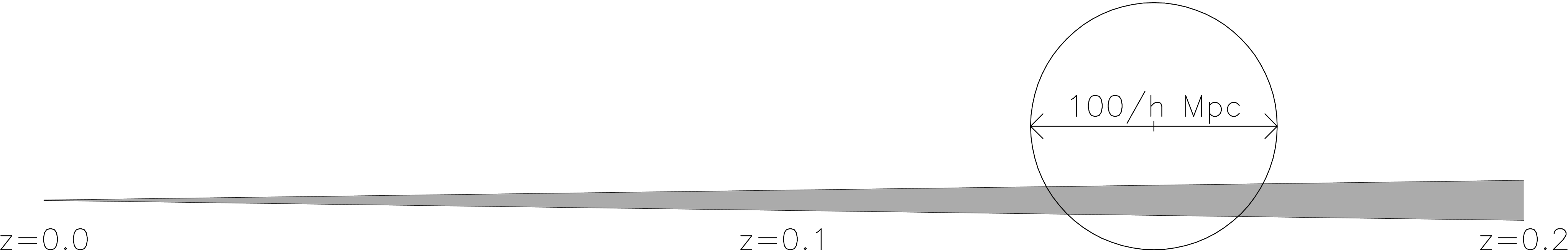
Figure 1: A schematic of the edge-on view of an LCRS slice (drawn to scale); at $z=0.2$, the width of an LCRS slice has grown to $\approx 15~{}h^{-1}$ Mpc. Also drawn to scale is a $100~{}h^{-1}$ Mpc-diameter sphere randomly intersecting the LCRS slice.

On very large scales ($~{}\hbox to0.0pt{$>$\hss}{\lower 4.30554pt\hbox{$\sim$}}50~{}h^{-1}$ Mpc), it makes sense to think of an individual LCRS slice as a 2-dimensional plane, since the third dimension of slice width does not contribute much to our understanding of clustering on these scales (Fig. 1). Now consider a “toy” Universe composed of osculating spherical voids of diameter $100~{}h^{-1}$ Mpc. In such a Universe, an LCRS slice would intersect several voids at various random positions. Clearly, the measured cross-sectional diameters of these intersections will never overestimate the true diameter of the spheres (in this case, $100~{}h^{-1}$ Mpc). On average, the diameter of the cross-section of a sphere randomly intersecting a plane is

$$<D_{\rm cross-section}>=\frac{\pi}{4}D_{\rm sphere}\approx\frac{3}{4}D_{\rm sphere}.$$ (1)

Thus, in such a “toy” Universe, we would expect that an LCRS slice would typically underestimate the average void diameter by about $1/3$. This projection effect in real space is basically the same as the aliasing of power from large- to small-scales in Fourier space. In real-space, however, this effect seems rather more benign and correctable.

With the above discussion in mind, what – if any – clustering do we see on scales of 50 – 200$~{}h^{-1}$ Mpc?

Figure 2: The LCRS Slice at $-12^{\circ}$. Only LCRS galaxies in the official redshift sample and within the absolute magnitude range $-22.5\leq M_{\rm R}-5\log h<-17.5$ are plotted.

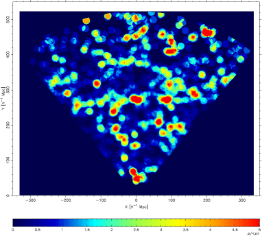
Figure 3: Smoothed density contrast map of the LCRS $-12^{\circ}$ Slice. Smoothing was performed with a $20~{}h^{-1}$ Mpc-diameter tophat filter. The $xy$-coordinates are in comoving distances.

First, consider a couple visual representations of the LCRS $-12^{\circ}$ Slice, the most densely and most homogeneously sampled of the six LCRS slices. Looking at a standard velocity-RA plot of this slice (Fig. 2), we may notice that the largest coherent high-contrast structures tend to form the walls of underdense regions (“voids”) 50 – 100$~{}h^{-1}$ Mpc in diameter. To remove radial and field-to-field selection effects, one can generate a smoothed number-density contrast map (Fig. 3); therein, our initial suspicions are confirmed: high-density ($\delta\rho/\rho~{}\hbox to0.0pt{$>$\hss}{\lower 4.30554pt\hbox{$\sim$}}2.5$) regions tend to surround low-density ($\delta\rho/\rho~{}\hbox to0.0pt{$<$\hss}{\lower 4.30554pt\hbox{$\sim$}}1$) “voids” with diameters of 50 – 100$~{}h^{-1}$ Mpc.

Second, we note that both the LCRS 2D power spectrum [5] and large-scale ($>10~{}h^{-1}$ Mpc) 3D spatial autocorrelation function [10] indicate features of excess clustering on scales $\sim 100~{}h^{-1}$ Mpc. We note that the results from the 2D power spectrum show higher statistical significance, since the signal at these scales (see Fig. 1) is essentially 2D; at these scales, some of the signal is washed out in the 3D autocorrelation function analysis.

Third, Doroshkevich et al.’s core-sampling analysis [2] of the LCRS measures the mean free path between 2D sheets and between 1D filaments. Comparing [2]’s Fig. 12 with our Fig. 3, it is apparent that their sheet-like structures correspond roughly with regions of smoothed $\delta\rho/\rho~{}\hbox to0.0pt{$>$\hss}{\lower 4.30554pt\hbox{$\sim$}}2.5$; their rich filaments, with regions of smoothed $1.5~{}\hbox to0.0pt{$<$\hss}{\lower 4.30554pt\hbox{$\sim$}}\delta\rho/\rho~{}\hbox to0.0pt{$<$\hss}{\lower 4.30554pt\hbox{$\sim$}}2$. Doroshkevich et al. measure the mean free path between sheets to be $\approx$ 80 – 100 $h^{-1}$ Mpc [2].

Fourth, Einasto et al. give evidence that Abell Clusters in rich superclusters tend to lie within a 3D “chessboard” of gridsize of $\sim 120~{}h^{-1}$ Mpc [3]. Einasto and his colleagues are presently performing a similar analysis for LCRS galaxies in rich environments [4]; in fact, our Fig. 3 is from the early stages of that analysis. Results, however, are still pending.

3 Conclusions

There does seem to be something going on in the LCRS at a scale of $\sim 100~{}h^{-1}$ Mpc, but this result needs confirmation using other techniques (e.g., a 2D $\xi_{\rm gg}$) and using other large surveys covering different regions and/or having different selection effects (e.g., the ESP [11], 2dF [1], SDSS [8], …).

Acknowledgements.  We wish to thank the following for fruitful discussions regarding the topic of this paper: Andrei Doroshkevich, Jaan Einasto, Richard Fong, Yasuhiro Hashimoto, Robert Kirshner, Stephen Landy, Augustus Oemler, and Paul Schechter.

References

- [1] Colless M.M., this volume
- [2] Doroshkevich A.G., Tucker D.L., Oemler A., Kirshner R.P., Lin H., Shectman S.A., Landy S.D., & Fong R., 1996, MNRAS, 283, 1281
- [3] Einasto J., Einasto M., Gottlöber S., et al., 1997, Nature, 385, 139
- [4] Einasto J., et al. 1998, in preparation
- [5] Landy S.D., Shectman S.A., Lin H., Kirshner R.P., Oemler A., & Tucker D., 1996. ApJL 456, 1
- [6] Lin H., Kirshner R.P., Shectman S.A., Landy S.D., Oemler A., Tucker D.L., & Schechter P.L., 1996a, ApJ, 464, 60
- [7] Lin H., Kirshner R.P., Shectman S.A., Landy S.D., Oemler A., Tucker D.L., & Schechter P.L., 1996b, ApJ, 471, 617
- [8] Loveday J., & Pier J., this volume
- [9] Shectman S.A., Landy S.D., Oemler A., Tucker D.L., Lin H., Kirshner R.P., & Schechter P.L., 1996, 470, 172
- [10] Tucker D.L., Oemler A., Kirshner R.P., et al., 1997, MNRAS, 285, 5.
- [11] Vettolani G., Zucca E., Zamorani G, et al., 1997, A&A, 325, 954