Non-linear dynamics of Kelvin-Helmholtz unstable magnetized jets: three-dimensional effects

Abstract

A numerical study of the Kelvin-Helmholtz instability in compressible magnetohydrodynamics is presented. The three-dimensional simulations consider shear flow in a cylindrical jet configuration, embedded in a uniform magnetic field directed along the jet axis. The growth of linear perturbations at specified poloidal and axial mode numbers demonstrate intricate non-linear coupling effects. The physical mechanims leading to induced secondary Kelvin-Helmholtz instabilities at higher mode numbers are identified. The initially weak magnetic field becomes locally dominant in the non-linear dynamics before and during saturation. Thereby, it controls the jet deformation and eventual breakup. The results are obtained using the Versatile Advection Code [G. Tóth, Astrophys. Lett. & Comm. 34, 245 (1996)], a software package designed to solve general systems of conservation laws. An independent calculation of the same Kelvin-Helmholtz unstable jet configuration using a three-dimensional pseudo-spectral code gives important insights into the coupling and excitation events of the various linear mode numbers.

I Introduction

The Kelvin-Helmholtz (KH) instability is a basic hydrodynamic phenomenon in sheared flows [1, 2]. Magnetic fields can strongly influence the linear and non-linear behavior of this instability. A recent full parameter study [3] (Paper I) of the growth and saturation of the KH instability in two-dimensional (2D) compressible magnetohydrodynamics (MHD) augmented the vast body of knowledge on magnetically induced effects [4, 5, 6, 7, 8, 9, 10, 11]. It illustrated how a weak, uniform B field gets amplified by the developing vortical flow and how this in turn changes the redistribution of mass as compared to pure hydrodynamic cases. Figure 1, taken from Paper I, shows a close-up of the density pattern after four transverse sound travel times in a magnetically modified KH evolution. Parameter values are listed below in section II B. The magnetic field becomes dynamically dominant at the time shown, halting the further growth in the transverse $y$-direction. The $x$-direction is periodic, so Fig. 1 shows alternating regions of density enhancements (bright) and depletions (dark). The narrow lanes of low density intersecting the high density regions signal sites of strong magnetic fields.

The KH instability is important for numerous astrophysical applications. Shear flows occur in jets ejected from star forming regions, in stellar winds, in winds emanating from accretion disks, …Many of the jet-type astrophysical flows are at such high speeds that the dominant dynamics is through shock interaction both internal to the jet and at its leading working surface where the jet penetrates the ambient plasma. The fundamental shear-induced instabilities that can develop at the jet surface are ultimately responsible for entrainment and mixing with the ambient material. Recently, Bodo et al. [12] performed comparative 2D and 3D hydrodynamic simulations of supersonic (Mach 10) jets. In their 3D simulations of a jet, 10 times less dense than its environment, faster decay into small-scale structure was demonstrated, as well as strong mixing with the external medium. The evolution was governed by the formation of internal shocks, induced external shocks, and consequent momentum and material mixing processes. Usually, the initial perturbation in 2D and 3D studies of this kind consists of a superposition of all linear wave modes, mimicking the dynamics resulting from random excitations. It is then very difficult to disentangle what causes the separate modes to couple. Therefore, we take a different approach and perturb at selected mode pairs. Our aim is to clearly identify cause and effect in the non-linear dynamics.

Typically, highly collimated jets are seen as bipolar outflows from young stellar objects. It is generally believed that the magnetic field plays an as yet not fully understood role in this collimation. Insights from 2D simulations have been carried over to 2.5 dimensions [5, 9, 13]. Numerical, fully three-dimensional calculations of astrophysical phenomena involving shear flow and magnetic fields consider MHD simulations of relativistic jets in aligned [14] and oblique magnetic fields [15], and have focused on density effects in poloidally magnetized supermagnetosonic jets [16]. In contrast to these studies where the long-term coherence of the jet is of interest, we assess initial transient features and the way in which Lorentz forces can saturate and control the jet deformation and breakup. We highlight this role played by magnetic fields in a simple cylindrical jet configuration with a uniform field parallel to the shear flow. Our study of 3D jets looks at these magnetic effects in the subsonic Kelvin-Helmholtz unstable regime. We concentrate on the three-dimensional non-linear hydrodynamic and magnetic effects. Due to the large computational cost required for 3D simulations, we restrict ourselves to two cases which are an immediate 3D generalization of the 2D case shown in Figure 1. The governing parameters [3] are chosen such that (i) the magnetic field is weak initially, allowing the hydrodynamic Kelvin-Helmholtz instability to develop; and (ii) the shear flow strength corresponds to its most unstable value in 2D in the sense that the saturation level is highest at fixed axial mode number. This axial wave number is taken close to, but slightly below the most unstable linear mode from the 2D case. By setting the mode number in the azimuthal direction we can investigate the influence of the three-dimensional geometry.

In this parameter regime, we can simulate the dynamics using two entirely different numerical tools: the general finite-volume based Versatile Advection Code (VAC [17, 18]), and the combined finite-difference, spectral code HEating by Resonant Absorption (HERA [19, 20]). While the latter is designed for magnetized loop dynamics involving strong radial gradients only, the former offers a choice of high-order, shock-capturing schemes typically used in computational fluid dynamics calculations. Of these two codes, only VAC is able to investigate the supersonic regime relevant for astrophysical jets. In this combined VAC-HERA study of the subsonic regime, we not only verify both codes against eachother, but also get additional insight in the various spectral contributions to the dynamics.

The MHD equations, initial conditions, and the numerical tools used are discussed in section II. We limit the discussion of the non-linear dynamics to two cases that only differ in the perturbation applied to the KH unstable jet. Section III contains a detailed analysis of their saturation behavior and illustrates the role played by the magnetic field. We briefly comment on the further evolution. Conclusions are presented in section IV.

II Numerical modeling of the problem

The ideal MHD equations constitute a set of conservation laws. The eight partial differential equations govern the time evolution of mass density $\rho$, momentum density $\rho\mbox{\bf v}$, total energy density $e$, and magnetic induction B. Written in these conservative variables, we get

$$\frac{\partial\rho}{\partial t}+\nabla\cdot(\rho\mbox{\bf v})=0,$$ (1)

$$\frac{\partial(\rho\mbox{\bf v})}{\partial t}+\nabla\cdot[\rho\mbox{\bf v}\mbox{\bf v}+p_{tot}I-\mbox{\bf B}\mbox{\bf B}]=0,$$ (2)

$$\frac{\partial e}{\partial t}+\nabla\cdot(e\mbox{\bf v})+\nabla\cdot(p_{tot}\mbox{\bf v})-\nabla\cdot(\mbox{\bf v}\cdot\mbox{\bf B}\mbox{\bf B})=0,$$ (3)

$$\frac{\partial\mbox{\bf B}}{\partial t}+\nabla\cdot(\mbox{\bf v}\mbox{\bf B}-\mbox{\bf B}\mbox{\bf v})=0.$$ (4)

We introduced $p_{tot}=p+\frac{1}{2}B^{2}$ as the total pressure, and $I$ as the identity tensor. The thermal pressure $p$ is related to the energy density as $p=(\gamma-1)(e-\frac{1}{2}\rho v^{2}-\frac{1}{2}B^{2})$. We set the adiabatic gas constant $\gamma$ equal to $5/3$. Magnetic units are defined such that the magnetic permeability is unity.

A Numerical tools

The numerical 3D time-dependent calculation of the Kelvin-Helmholtz instability in magnetized plasma jets is done twice with two completely independent software tools, the Versatile Advection Code (VAC [17, 18]), and the HEating by Resonant Absorption code (HERA [19, 20]). Detailed descriptions of the algorithms employed in these codes are found through the references, here we only highlight the differences. VAC is more general in terms of algorithms [21, 22], applications [23, 24, 3, 25], and geometry, while HERA is truly specialized to the solution of the 3D MHD equations in cylindrical geometry [26, 20]. Both codes run on vector and distributed memory architectures, and their implementation and performance aspects are detailed elsewhere [27, 28]. The VAC and HERA results in this paper were obtained on a shared memory vector Cray C90 and on 16 processors of the Cray T3E and IBM SP.

VAC employs a finite volume discretization on a structured grid, while HERA uses finite differences in the radial direction, and a 2D spectral

$$\exp\left(im\varphi+in\frac{2\pi Z}{L}\right)$$ (5)

representation in the azimuthal direction ($\varphi$) and along the cylinder ($Z$). In VAC, we selected the explicit, one-step Total Variation Diminishing scheme [29] with Woodward limiting [30]. This scheme makes use of a Roe-type approximate Riemann solver [31]. The conservation form of the MHD equations is taken and ensured by this discretization. HERA uses a semi-implicit predictor-corrector time stepping algorithm [19] and advances the primitive variables $\rho$, v, $p$, and B. The discrete equivalent of $\nabla\cdot\mbox{\bf B}=0$ is ensured in VAC by applying a projection scheme at every time step [32] using an efficient iterative method. HERA instead uses a staggered radial mesh, which allows to encode a discretization that keeps the field divergence identically zero. For the HERA calculations reported in section III, we use a stabilizing ‘artificial viscosity’ term $\mu\nabla^{2}\mbox{\bf v}$ added to the momentum equation, with $\mu={\cal O}(10^{-4})$. For the resolutions used in the calculations, this turns out to be roughly at the order of the numerical dissipation inherent to the scheme used from VAC.

B Initial conditions

The 3D jet configuration generalizes the 2D simulation shown in Figure 1. This calculation started from a uniform density $\rho_{0}=1$, pressure $p_{0}=1$ and magnetic field $\mbox{\bf B}_{0}$ parallel to a shear flow of the form $v_{x}=0.645\tanh(y/0.05)$. The initial plasma beta was $\beta=2p_{0}/B^{2}_{0}\simeq 120$, and this 2D reference case is further characterized by the dimensionless sound Mach number $M_{s}=0.5$ (ratio of the shear flow amplitude to the sound speed) and Alfvén Mach number $M_{a}=5.0$ (ratio of shear flow amplitude to the Alfvén speed). Our previous study in two space dimensions [3] showed that for these parameters, the non-linear saturation level is maximal at the chosen sound Mach number for the mode with wave number $k=1$. Therefore we apply a perturbation to the shear flow according to $\delta v_{y}\sim\sin(2\pi x)$.

In 3D, we consider a jet-like flow. Using $(R,\varphi,Z)$ cylindrical coordinates, we set up a flow field

$$v_{Z}(R;t=0)=V_{0}\tanh\frac{R-R_{jet}}{a}$$ (6)

parallel to a cylinder of length $L=1$ and radius $R_{jet}=0.5$, which is sheared in the radial direction. Note that the jet surface $R=R_{jet}$ is easily identified as the $v_{Z}=0$ isosurface. The strength of the velocity shear is fixed at $V_{0}=0.645$, and the width of the shear layer is $a=0.1R_{jet}=0.05$ exactly like in the reference 2D case. Further, the initial pressure $p_{0}$ and density $\rho_{0}$ are equal to unity everywhere, and we impose a uniform initial field $\mbox{\bf B}=B_{0}\hat{e}_{Z}$ parallel to the jet. Taking $B_{0}=0.129$, we have a 3D configuration with identical properties as the reference KH unstable 2D case [3] shown in Fig. 1. We perturb the cylindrical jet surface by imposing a radial velocity profile

$$v_{R}(R,\varphi,Z;t=0)=\Delta v_{R}\exp{-\left(\frac{R-R_{jet}}{4a}\right)^{2}}\cos(m\varphi)\sin\frac{n2\pi Z}{L}.$$ (7)

Hence, we impose a perturbation at specific mode numbers $m$ and $n$. This does represent a truly 3D perturbation, as it translates into the simultaneous excitation of four 2D Fourier modes (5), namely $(+m,+n)$ with complex amplitude $-i/4$, $(+m,-n)$ with amplitude $+i/4$, and similarly for the $(-m,\pm n)$ modes (since the velocity is a purely real quantity). These symmetry considerations will allow us to refer to $(m,n)$ mode pairs with always $m\geq 0$ and $n\geq 0$, tacitly assuming the $(\pm m,\pm n)$ individual mode contributions. The amplitude of the perturbation is fixed at $\Delta v_{R}=0.01$ and its radial width is chosen to be $4a=0.2$.

C Boundary conditions

We calculate the evolution of the KH unstable jet with both VAC and HERA. For VAC, we set up the jet configuration in a Cartesian $(x,y,z)$ box of sizes $L\times 4R_{jet}\times 4R_{jet}$. Note the difference between the Cartesian $z$ and the cylindrical $Z$-direction. In fact, the first, periodic $x$-dimension is now along the jet. We assume outflow boundary conditions on the sides parallel to the jet. We take $L=1$ and an aspect ratio of $L/R_{jet}=2$. We use $50\times 100\times 100$ equidistant grid points.

For HERA, the jet is placed within a co-axial cylinder of radius $2R_{jet}$. We took $64$ radial grid points, and 32 modes both in the $\varphi$ and $Z$ dimensions. HERA naturally assumes periodic boundary conditions along ($Z$-direction) and about ($\varphi$-direction) the loop, while a regularity condition holds at $R=0$. We took a closed, perfectly conducting wall at the outer radius, which is the only difference in the problem setup between VAC and HERA. All calculations reported below are not (yet) influenced by this difference in ‘open box’ versus ‘closed cylinder’ outer boundary configuration.

III Non-linear dynamics in sheared jets

A Case $m=1$

Figure 2 shows the time evolution of the scaled poloidal kinetic and magnetic energies from both calculations when we perturb at mode numbers $m=1$ and $n=1$. These are volume integrated quantities, namely

$$E^{pol}_{mag}(t)\stackrel{{\scriptstyle\rm VAC}}{{=}}\frac{1}{B_{0}^{2}R_{jet}^{2}L}\int_{V}dV\,\frac{B_{y}^{2}+B_{z}^{2}}{2}\stackrel{{\scriptstyle\rm HERA}}{{=}}\frac{1}{B_{0}^{2}R_{jet}^{2}L}\int_{V}dV\,\frac{B_{R}^{2}+B_{\varphi}^{2}}{2},$$ (8)

and similarly

$$E^{pol}_{kin}(t)\stackrel{{\scriptstyle\rm VAC}}{{=}}\frac{1}{\rho_{0}V_{0}^{2}R_{jet}^{2}L}\int_{V}dV\,\rho\frac{v_{y}^{2}+v_{z}^{2}}{2}\stackrel{{\scriptstyle\rm HERA}}{{=}}\frac{1}{\rho_{0}V_{0}^{2}R_{jet}^{2}L}\int_{V}dV\,\rho\frac{v_{R}^{2}+v_{\varphi}^{2}}{2},$$ (9)

and they allow a determination of the growth rate and the saturation behavior of the instability. Note that the difference in the total volume of the simulated box (VAC) or cylinder (HERA) does not make a difference for these volume integrals since the functions are zero far from the jet surface.

The agreement between the finite volume based VAC code and the pseudo-spectral HERA code is excellent: the growth and saturation behavior is clearly captured at about $t=4$. The spectral code allows us to identify the contributions of all linear wave numbers $(m,n)$ at any particular moment in time. The contributions to the poloidal magnetic energy of the most dominant wave numbers are indicated in the figure. We immediately read off how the $(1,1)$ perturbations induce $(0,2)$, $(2,2)$, and $(2,0)$ modes, in that order. These couple and reverse their original ordering at $t\simeq 0.75$. At saturation $t=4$, the three most important mode number pairs are the excited $(1,1)$ and the induced $(3,1)$ and $(0,2)$ modes. Note that, interestingly, the $(m,m)$ modes with $m\geq 2$ of similar helicity as the excited $(1,1)$ mode never play an important role during and beyond the saturation phase, at least not for $t\leq 6$. This is in spite of the fact that they are excited fairly early on in the growth phase of the instability: the $(2,2)$ modes enter in the quasi-linear regime for $t<0.5$ (see Figure 2), and $(3,3)$, $(4,4)$, …pairs are among the first excited wave numbers. For times $t\leq 6$, they never amount to a significant contribution to the total poloidal magnetic energy.

While we now know which mode numbers are dominating the dynamics at any particular time, it remains to identify what causes their various couplings. In what follows, we sketch the physical mechanisms which trigger individual modes during the growth and saturation phase of the 3D KH instability. It should be clear that the combined finite volume and spectral calculations led us to a fairly detailed insight in the intricate non-linear dynamics.

Analytic results for quasi-linear regime

First, we can make some analytic predictions for times earlier than $t\simeq 0.5$, where the behavior is essentially ‘quasi-linear’. Since the initial plasma beta is high, $\beta(t=0)\approx 120$, we can neglect magnetic effects altogether during this phase. We employ a cylindrical coordinate system $(R,\varphi,Z)$ centered on the jet. The total velocity field can be written as a sum of the equilibrium shear flow, the imposed radial velocity perturbation, and an induced small velocity perturbation as follows:

$$\mbox{\bf v}(R,\varphi,Z;t)\simeq v_{0}(R)\,\hat{e}_{Z}+\Delta v_{R}(R)\,\cos{\varphi}\sin\frac{2\pi Z}{L}\,\hat{e}_{R}+\delta\mbox{\bf v}(R,\varphi,Z;t).$$ (10)

We then analyse the linear and most dominant non-linear effects in a pure hydrodynamic description. On the jet surface $R=R_{jet}$, $v_{0}(R_{jet})=0$ and $\Delta v_{R}(R_{jet})\gg\delta v_{R}(R_{jet})$. In the vicinity of this jet surface, we can safely assume that $\Delta v_{R}$ is constant. We start from the hydrodynamic equations, written in cylindrical coordinates, and employ primitive variables $\rho$, $p$, and v. The continuity equation in cylindrical coordinates is

$$\frac{\partial\rho}{\partial t}+v_{R}\frac{\partial\rho}{\partial R}+\frac{v_{\varphi}}{R}\frac{\partial\rho}{\partial\varphi}+v_{Z}\frac{\partial\rho}{\partial Z}+\rho\left[\frac{1}{R}\frac{\partial(Rv_{R})}{\partial R}+\frac{1}{R}\frac{\partial v_{\varphi}}{\partial\varphi}+\frac{\partial v_{Z}}{\partial Z}\right]=0.$$ (11)

Using expression (10), writing $\rho\equiv\rho_{0}+\delta\rho(R,\varphi,Z,t)$, $p\equiv p_{0}+\delta p(R,\varphi,Z,t)$, and evaluating at $R=R_{jet}$, we get:

$$\frac{D\rho}{Dt}+\rho\nabla\cdot\mbox{\bf v}=0 \ \ \ \Rightarrow\ \ \ \delta\rho\simeq-t\frac{\rho_{0}}{R}\Delta v_{R}\cos{\varphi}\sin\frac{2\pi Z}{L}+\ldots$$ (12)

$$\delta p=c_{0}^{2}\delta\rho \ \ \ \Rightarrow\ \ \ \delta p\simeq-t\frac{\gamma p_{0}}{R}\Delta v_{R}\cos{\varphi}\sin\frac{2\pi Z}{L}+\ldots$$ (13)

where $c_{0}=\sqrt{\gamma p_{0}/\rho_{0}}$ is the sound speed for the unperturbed configuration.

Hence, the linear pressure perturbation on the jet surface, in phase with the density perturbation, follows immediately from the non-vanishing radial divergence of the imposed perturbation through the term $\frac{1}{R}\frac{\partial}{\partial R}(Rv_{R})$. All other terms in equation (11) lead to ${\cal O}\left(\Delta v_{R}\,t^{2}\right)$ contributions, which enter the dynamics later.

In the $\varphi$-component of the momentum equation,

$$\frac{\partial v_{\varphi}}{\partial t}+v_{R}\frac{\partial v_{\varphi}}{\partial R}+\frac{v_{\varphi}}{R}\frac{\partial v_{\varphi}}{\partial\varphi}+v_{Z}\frac{\partial v_{\varphi}}{\partial Z}+\frac{v_{R}v_{\varphi}}{R}=-\frac{1}{R\rho}\frac{\partial p}{\partial\varphi},$$ (14)

the dominant term at $R=R_{jet}$ is the linearly induced pressure gradient in the $\varphi$-direction, so using (13) we get:

$$\frac{\partial\delta v_{\varphi}}{\partial t}=-tc^{2}_{0}\frac{\Delta v_{R}}{R^{2}_{jet}}\sin{\varphi}\sin\frac{2\pi Z}{L}+\ldots$$ (15)

Similarly, the longitudinal velocity $v_{Z}$-component at $R=R_{jet}$ is dominated by purely linear effects, but it has two distinct contributions. The full equation is

$$\frac{\partial v_{Z}}{\partial t}+v_{R}\frac{\partial v_{Z}}{\partial R}+\frac{v_{\varphi}}{R}\frac{\partial v_{Z}}{\partial\varphi}+v_{Z}\frac{\partial v_{Z}}{\partial Z}=-\frac{1}{\rho}\frac{\partial p}{\partial Z}.$$ (16)

Again, the induced pressure gradient term along $Z$ contributes, but now also the shear in the background flow profile has a linear term associated with it, such that

$$\frac{\partial\delta v_{Z}}{\partial t}\simeq-\Delta v_{R}\cos{\varphi}\sin\frac{2\pi Z}{L}\left.\frac{dv_{0}}{d\,R}\right|_{R_{jet}}+tc^{2}_{0}\frac{\Delta v_{R}}{R_{jet}}\frac{2\pi}{L}\cos{\varphi}\cos\frac{2\pi Z}{L}+\ldots$$ (17)

So far, all terms considered are purely linear. The quasi-linear effects enter by a consideration of the equation for the radial velocity,

$$\frac{\partial v_{R}}{\partial t}+v_{R}\frac{\partial v_{R}}{\partial R}+\frac{v_{\varphi}}{R}\frac{\partial v_{R}}{\partial\varphi}+v_{Z}\frac{\partial v_{R}}{\partial Z}-\frac{v_{\varphi}^{2}}{R}=-\frac{1}{\rho}\frac{\partial p}{\partial R}.$$ (18)

Close to the jet surface, the appropriate ordering of terms becomes

$$\frac{\partial\delta v_{R}}{\partial t}=-\frac{1}{\rho_{0}}\frac{\partial\delta p}{\partial R}-\delta v_{Z}\Delta v_{R}\frac{2\pi}{L}\cos{\varphi}\cos\frac{2\pi Z}{L}+\frac{\delta v_{\varphi}}{R_{jet}}\Delta v_{R}\sin\varphi\sin\frac{2\pi Z}{L}+\frac{(\delta v_{\varphi})^{2}}{R_{jet}}+\ldots$$ (19)

The non-linear effects arise from the $\mbox{\bf v}\cdot\nabla\mbox{\bf v}$ terms. We can approximate (19), using the linear terms in the expressions (13), (15) and (17), as

$$\frac{\partial\delta v_{R}}{\partial t} \simeq t\,\Delta v_{R}\frac{c^{2}_{0}}{R^{2}_{jet}}\cos{\varphi}\sin\frac{2\pi Z}{L}+t\,(\Delta v_{R})^{2}\frac{dv_{0}}{dR}_{\mid R_{jet}}\frac{\pi}{2L}\left[\sin\frac{4\pi Z}{L}+\cos(2\varphi)\sin\frac{4\pi Z}{L}\right]$$ (20)

$$- t^{2}(\Delta v_{R})^{2}\frac{c^{2}_{0}}{2R_{jet}}\left[\frac{4\pi^{2}}{L^{2}}\cos^{2}{\varphi}\cos^{2}\frac{2\pi Z}{L}+\frac{1}{R^{2}_{jet}}\sin^{2}{\varphi}\sin^{2}\frac{2\pi Z}{L}\right]+{\cal O}\left\{t^{4}(\Delta v_{R})^{2}\right\}$$ (21)

Hence, the $(1,1)$ excitation leads to $(0,2)$, $(2,2)$ contributions in the quasi-linear regime. The third term in expression (LABEL:q-vr2) has a $(2,0)$ effect in it as well, since $\cos^{2}\alpha=(\cos(2\alpha)+1)/2$. The quasi-linear analytic reasoning thus validates the observed ordering in time in the first-excited linear mode numbers as seen in Fig. 2. At the same time, we identified the physical effects that cause their excitation.

Excitation of secondary KH instabilities

Beyond this quasi-linear phase, the physical interpretation of various non-linear coupling events must be guided by the numerical solutions calculated with both codes. Following Fig. 2, it remains to identify why, in addition to the excited $(1,1)$ modes, the $m=3$ and $n=2$ wave numbers govern the dynamics at the time of saturation at $t\approx 4$. Moreover, the influence of the magnetic field needs to be discussed. This is best illustrated using the picture gallery shown in Fig. 3.

The first frame A shows the density perturbation at $t=4$ in a horizontal cutting plane through the jet axis. The sinusoidal, sideways $(1,1)$ displacement of the jet essentially reduces to a ‘doubled’ 2D simulation in this plane. Indeed, at each of both intersections with the jet surface we created initial conditions much like those used for the 2D result shown at saturation in Fig. 1. The 3D result shows that the basic features are unaltered: vortical flow has redistributed mass along the direction of the jet in periodic depletions (dark regions) and enhancements (bright). At the center of those regions where mass is accumulated, a narrow lane of low-density is formed which coincides with high magnetic fields, as the field gets entrained and compressed by the global plasma circulation. There is a significant difference with the 2D result, namely that the positioning of the resulting saturation pattern is shifted along the jet axis. In the pure 2D simulation from Fig. 1, the induced vertical pressure gradient $\frac{d\delta p}{dy}$ is in phase with the initial vertical velocity perturbation $\delta v_{y}\sim\sin{2\pi x}$. The shear background flow introduces a force within the shear layer which is purely along the $x$-direction. The quasi-linear analytic treatment presented above clearly shows in equation (17) how an extra pressure gradient term, out of phase with the imposed velocity perturbation, enters the description. As a result, the observed axial shift of the pattern ensues.

Frame B in Fig. 3 shows the same horizontal cut in a 3D view of the simulation domain, and a specific high-density isosurface where $\rho=1.07$. The actual range in density is now $[0.73,1.11]$. Note how the high density zones appear as two ‘banana’-shaped surfaces at diagonally opposing positions with respect to the center of the box. The density perturbation is thus clearly dominated by a $(1,1)$ mode number pair. The enhanced density regions coincide with zones of excess pressure, according to equation (12). This is best demonstrated by visualizing the jet surface $v_{x}=0$, and coloring it with its local thermal pressure. This is done in frame C of the picture gallery. Note the diametrically opposing high pressure zones (bright) in the same location as the high density regions, and similarly for the low pressure (or density) regions along the other diagonal. For the particular aspect ratio of the simulated jet, the resulting poloidal pressure gradient in the $\varphi$-direction on the jet surface has induced a particular poloidal flow pattern on top and bottom of the jet surface. This flow essentially wraps the high pressure regions around top and bottom of the jet surface, thereby invading the low pressure zones. This occurs along the positive $y$-direction in the front half of the jet, and along the negative $y$-direction at the back half. This effectively doubles the axial mode number $n$ of the perturbation along top and bottom of the jet. If we make a vertical cut through the density structure containing the jet axis, as in frame D of Fig. 3, an induced $n=2$ KH perturbation is clearly visible.

Role of the magnetic field at saturation

So far, the role of the magnetic field is not fully explained. However, at saturation $t=4$, the plasma beta is locally reduced to $\beta\approx 4.96$ from the initially uniform $\beta(t=0)\approx 120$, while the Alfvénic Mach number $M_{a}$ is as low as $0.01$. Magnetic effects can no longer be ignored. The induced flow pattern causing the excitation of a $n=2$ KH perturbation at top and bottom of the jet also entrails the field lines. Frame E in Figure 3 shows the $\log_{10}(B^{2}_{pol})=-1.4$ isosurfaces of the squared poloidal magnetic field strength, which was zero at $t=0$. These are cospatial with the strongest total magnetic field zones, and four distinct regions are visible: two sheet-like structures at the positions where the density is enhanced, and two curly fibril structures along top and bottom of the jet. The sheet structures are the immediate 3D generalization of the low-density, high-field lanes visible in the 2D calculation shown in Fig. 1. Note how they coincide with a central low-density zone within the ‘banana’ high density isosurface from frame B. The fibril structures are high field regions built up by the induced flow pattern around top and bottom of the jet, discussed earlier. They coincide with low pressure, low density regions with a similar 3D curved shape. In fact, the vertical cut of the density structure from frame D contains three intersections of the actual 3D low density fibril at each jet crossing. Just as in 2D, the magnetic field has become locally dominant in the dynamics, and thereby saturates the instability and controls the further evolution. The final frame illustrates this clearly, where we now visualize the velocity field in a vertical cut perpendicular to the jet axis at $x=0.5$. The arrows indicate the poloidal velocity field, and a clear circulation is seen about the high field fibrils. The contours of the $x$-component of vorticity are also showing the same effect. The thick solid line is the $v_{x}=0$ jet surface, which has a clear $m=3$ perturbation in it. Hence, the thermal pressure and the magnetic field cooperate to induce $n=2$ and $m=3$ contributions that dominate the saturation behavior along with the $(1,1)$ initial disturbance. The resulting density variation in three space dimensions is shown in Fig. 4, and can now be interpreted from the preceding exposition.

B Case $m=2$

Figure 5 shows the development and saturation behavior of the KH unstable jet, when the initial excitation has a $\cos{2\varphi}\sin{2\pi Z/L}$ variation. Figure 6 gives a 3D impression of the density variation at $t=4$ for this case, and there is significant fine structure in all spatial directions.

The information on the excitation and coupling events between linear modes can again be extracted directly from the HERA calculation, and used for the physical interpretation of the non-linear dynamics. A quasi-linear description, completely analogous to the one for $m=1$, predicts the initial excitation of the $(0,2)$, $(4,2)$, and $(4,0)$ modes. The later evolution and saturation is dominated by the imposed $(2,1)$ and the excited $(4,0)$ mode pair. The discussion of the simpler $m=1$ case in terms of pressure-gradient induced effects and the role of the magnetic field can be carried over to the present configuration. Note that the initial $(2,1)$ perturbation leads to four distinct zones where flows converge, building up high density, high pressure regions. Instead of the two diagonally opposing regions as shown in frame B of Figure 3, we now have two regions in the front half of the jet $0<x<0.5$, and two in the back half $0.5<x<1$. The front two are at the top and the bottom of the jet, with the back ones at the left and right edge. Figure 6 shows three of the enhanced density zones (bright) using various cutting planes through the simulation box at $t=4$. As a result of the associated pressure variations about the jet surface, flows are set up which again entrail magnetic field lines. As a direct generalization of frame E in Figure 3, one ends up with sheets of high magnetic fields intersecting the four compression zones, and a set of four fibril structures curled in between these zones as a secondary effect from the pressure induced flows. The effects on the density structure are well represented in Figure 6. Values range from $0.77$ to $1.10\,$.

C Further evolution

The evolution beyond the non-linear saturation is governed by many more mode numbers, as clearly seen in Figures 2-5. The regions where the magnetic field dominates essentially break up the jet, as identified by its $v_{x}=0$ isosurface. A transition to more turbulent flow sets in, but quantitative statements about this transition would require higher resolution 3D studies. These must assess the role played by numerical dissipation, not only in the way it affects the momentum evolution (viscous effects), but also in the developing fine-scale magnetic field (through resistive studies). A combined approach, like the simultaneous finite volume and spectral calculations presented here, will certainly help in sorting out physics from possible numerical artefacts.

IV Conclusions

Both the $m=1$ and the $m=2$ case study concentrated on the growth and saturation phase of KH unstable sheared magnetized jets. For the chosen parameters, a detailed account of the non-linear excitation of several $(m,n)$ 2D Fourier modes was presented. The combined finite volume and spectral calculations allowed for an in-depth analysis of the physical mechanisms behind non-linear mode couplings. The initially weak magnetic field could be ignored to make analytic predictions about the initial excitation of several mode pairs during the quasi-linear phase. The field eventually becomes locally dominant, and controls the 3D density structure at saturation. At the particular aspect ratio $L/R_{jet}=2$, we saw how an $(m,n)=(1,1)$ kink perturbation of the jet leads to a secondary KH instability, characterized by an axial $n=2$ wave number, along top and bottom of the jet. The induced poloidal pressure gradient triggers this instability. The magnetic field gets compressed in narrow sheets that intersect $(1,1)$ compression zones, and in 3D fibrils due to these secondary KH flows. These, in turn, cause an $m=3$ deformation of the jet surface. Similar effects were present in the $(m,n)=(2,1)$ case study.

Clearly, the initial plasma beta, the strength of the shear flow, and the aspect ratio of the jet all play an important role in this process. A detailed parameter study should explore their influence, along the lines of previous 2D studies [3]. The particular choice of parameter values used here (subsonic, high beta) could occur in the lower atmospheric regions of stars like our Sun: the high beta photospheric and chromospheric layers possess a variety of magnetically modified, shear flow regimes. We can safely speculate that magnetic effects will be important in highly supersonic, extragalactic jets as well. Initially weak fields can become locally dominant, e.g. through shock compression. In turn, the field may then dictate the type of shock interactions possible to the flow. Future investigations can look at specific geometries (flaring flux tubes, solar coronal loops) and adjust field strengths, shear strengths, include gravitation, etc. Instead of a uniform, weak B field parallel to the jet, the initial magnetic field configuration could contain current sheet(s). It is then possible to investigate tearing unstable situations in conjunction with background shear flows. Such effects have recently been studied in 3D incompressible MHD calculations of a magnetized wake [33] for studying the slow component of the solar wind. The effects of compressibility, which we analyzed for cases whithout initial current sheets, should be quantified in subsequent work.

Figure Captions:

Figure 1: The density structure after four transverse sound travel times, in a magnetically modified 2D Kelvin-Helmholtz evolution. At this time, the instability is non-linearly saturated. Dark lanes of low density where the magnetic field is intensified intersect high density (bright) regions, as seen at the periodic edges.

Figure 2: The time history of the scaled poloidal kinetic $E^{pol}_{kin}(t)$ ($\times 10$, thick dashed) and magnetic $E^{pol}_{mag}(t)$ (thick solid) energy, for the $m=1=n$ case, from both the VAC and the HERA calculations. The growth and the non-linear saturation as identified by the first maximum in $E^{pol}_{kin}(t)$ agree closely. The contributions from the most important individual mode number pairs $(m,n)$ to $E^{pol}_{mag}(t)$ are plotted as well, and the linestyle varies with the azimuthal mode number $m$: thin solid for $m=0$ (or $m\geq 6$), dotted $m=1$, thin dashed $m=2$, dash-dotted $m=3$, $-\cdot\cdot\cdot-$ for $m=4$, long dashes $m=5$.

Figure 3: Picture gallery for the $m=1$ case at saturation $t=4$. Frame (A): the density structure in a horizontal cut through the jet axis, to be compared to the 2D case in Figure 1. (B): the same cut as in frame (A), with the $\rho=1.07$ high density isosurface. Frame (C): the deformed jet surface $v_{x}=0$, colored with thermal pressure. Frame (D): the density structure in a vertical cut containing the jet axis, demonstrating the induced $n=2$ KH instability at top and bottom of the jet. (E): $\log_{10}(B^{2}_{pol})=-1.4$ isosurfaces, showing the locations of magnetic field dominated dynamics. Frame (F): a vertical cut perpendicular to the jet axis, showing the poloidal flow field as vectors, the $v_{x}=0$ jet surface as a thick solid line, and contours of $(\nabla\times\mbox{\bf v})_{x}$.

Figure 4: A rotated view of the 3D density structure for the $m=1$ case at saturation $t=4$. The dark regions are sites of low density, resulting from dynamically strong magnetic fields.

Figure 5: As in Figure 2, for the $m=2$ case.

Figure 6: The $m=2$ equivalent of Figure 4.

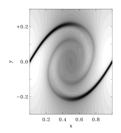
FIG. 1.:

FIG. 2.:

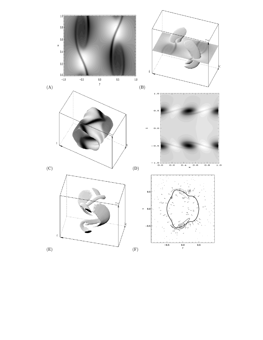
FIG. 3.:

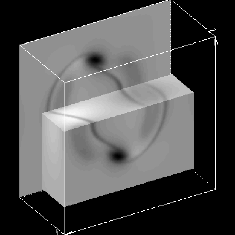
FIG. 4.:

FIG. 5.:

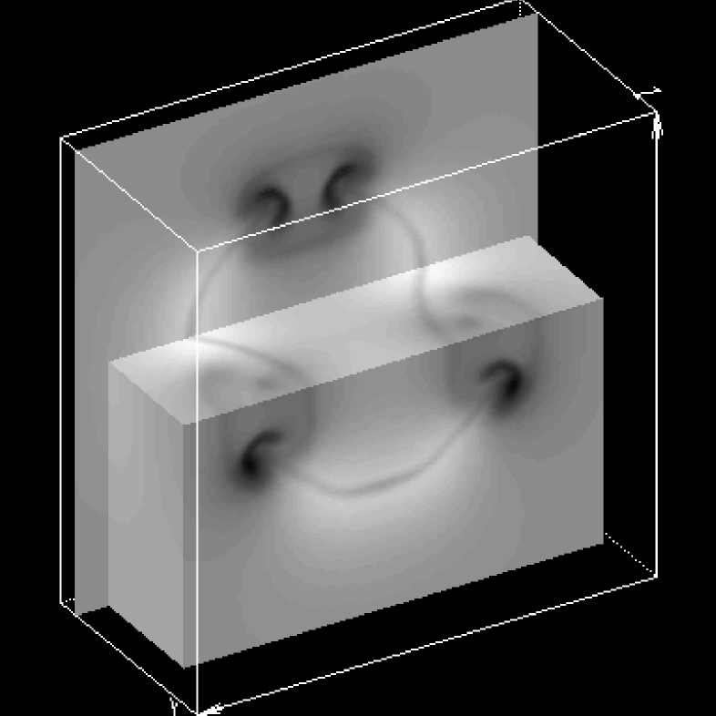
FIG. 6.: