Microlensing Optical Depth of the Large Magellanic Cloud

Abstract

The observed microlensing events towards the lmc do not have yet a coherent explanation. If they are due to Galactic halo objects, the nature of these objects is puzzling — half the halo in dark $0.5\;M_{\odot}$ objects. On the other hand, traditional models of the lmc predict a self-lensing optical depth about an order of magnitude too low, although characteristics of some of the observed events favor a self-lensing explanation. We present here two models of the lmc taking into account the correlation between the mass of the stars and their velocity dispersion: a thin Mestel disk, and an ellipsoidal model. Both yield optical depths, event rates, and event duration distributions compatible with the observations. The grounds for such models are discussed, as well as their observational consequences.

Galaxy: halo, kinematics and dynamics, stellar content – Cosmology: dark matter, gravitational lensing

1 Introduction

One of the greatest uncertainties in the interpretation of the microlensing events detected towards the Large and the Small Magellanic Clouds by the macho (Alcock et al. 1997a, Alcock et al. 1997b ) and the eros experiments (Renault et al. 1997, Palanque-Delabrouille et al. 1998) resides in the determination of the location and consequently of the nature of the lenses.

The macho results can be converted into an optical depth of $2.9_{-0.9}^{+1.4}\times 10^{-7}$, while the two candidate events of eros would account for $\sim 0.8\times 10^{-7}$. Combining both results leads to an average optical depth of $2.1_{-0.8}^{+1.3}\times 10^{-7}$ (Bennett (1998)).

While this observed optical depth towards the lmc is too small to account for a full dark halo of compact objects (expected $\tau=5\times 10^{-7}$), it is much too large to be explained by the contribution from known populations of low-mass stars in the disks of the Milky Way and the lmc: based on star counts, the contribution from the disk of our Galaxy is found to be $\tau_{\rm MW}\sim 8\times 10^{-9}$ (Gould et al. (1997)), and the global rate from known stars in both galaxies has been estimated by several authors to be $\lesssim 20\%$ (Wu (1994), Sahu (1994), de Rújula et al. (1995)) of that observed.

Moreover, the location of a few lenses has been determined, either through the non-detection of parallax effect for 97-SMC-1 (Palanque-Delabrouille et al. (1998)), or through the observation of the caustic crossing in the case of binary lenses, for 98-SMC-1 (Afonso et al. 1998, Albrow et al. (1999), Alcock et al. (1999), Rhie et al. 1999, Udalski et al. 1999) or MACHO-LMC-9 (Bennett et al. 1996). The case for the latter is still unclear however, since the measured lens velocity, incompatible with a Galactic halo lens unless the source happens to be a binary star with the appropriate separation, seems too low for a lmc disk star.

It has been pointed out by several authors (Kerins & Evans 1999, Di Stefano (1999)) that the fact that the observed binary lenses are all located in the Clouds might indicate that all observed events arise from Clouds deflectors. Indeed, if the two observed binary lenses with caustic crossings are in the Clouds, then the expected number of self-lensing caustic crossing events has to be greater than .53 at 90% C.L. A very conservative estimate of the fraction of caustic crossing events (Mao & Paczińsky (1991), Di Stefano (1999)) implies that we expect more than 5 background self-lensing events, which is far from negligible as compared to the total number of observed events.

The case for self-lensing in the lmc and smc is thus still open, despite the “proof” (Gould (1995)) that its contribution to the optical depth is too low. As shown in (Palanque-Delabrouille et al 1998), the smc could be thick enough to yield an expected optical depth as large as $\sim 2\times 10^{-7}$, compatible with the current observations towards this line-of-sight. A more thorough exploration of possible lmc models therefore appears worthwhile.

Gould (1995) noticed that the optical depth associated to the self-lensing of a stellar disk, a good approximation for the bulk of the lmc matter, depends only on the vertical velocity dispersion $\sigma_{W}$ of the stars:

$$\tau_{\mathrm{\mathsc{lmc}}}\;=\;2\,\frac{\sigma_{W}^{2}}{c^{2}}\,{\rm sec}^{2}i\;\;,$$ (1)

where $i$ is the inclination of the disk. Measurements of stellar velocities in the lmc are difficult because of its distance. Only the brightest stars are resolved. Gould based his analysis on the CH objects studied by Cowley & Hartwick (1991). These carbon stars belong to the asymptotic giant branch (AGB) of the HR diagram. With an apparent magnitude $m_{\rm bol}\sim 14-15$ and assuming a distance modulus of 18.6, their bolometric luminosities are in the range $2-5\times 10^{3}\;L_{\odot}$. A velocity dispersion of $\sim$ 20 km/s led Gould to the conclusion that the optical depth for lmc self-lensing could not exceed $1.1\times 10^{-8}$, well below the measured value of $1-3\times 10^{-7}$. However, carbon stars are a peculiar population. They have left the main sequence (ms) on which they have spent at most $\sim 10-12$ Gyr, the age of the lmc. The average lifetime of a star on the ms decreases with the initial stellar mass $m$ as

$$t_{\rm\mathsc{ms}}\simeq\left(1.2\times 10^{10}\;{\rm yr}\right)\,\left(m\;[M_{\odot}]\right)^{-3}\;\;,$$ (2)

so that the oldest carbon stars observed today had an initial mass larger than $\sim$ 1 $M_{\odot}$. Assuming a Salpeter imf for the lmc (Geha et al. 1998) and adopting the star formation history derived by the same authors lead to the conclusion that approximatively 75 % of the sample analyzed by Cowley & Hartwick (1991) has formed less than 2 Gyr ago, during a recent stellar burst. The velocity dispersion of 20 km/s refers therefore to young objects whereas the bulk of the lmc population is not dominated by young stars (Geha et al. 1998) and could be associated to much larger velocity dispersions. As a matter of fact, Hughes et al. (1991) have measured the radial velocities of long period variables (LPV) in the lmc and showed that while young and intermediate LPV’s had a dispersion velocity in the range between 12 and 25 km/s, the old LPV’s had a significantly larger dispersion velocity ranging from 31 to 45 km/s.

The increase of the velocity dispersion with the age of stars is a well-known fact. Bienaymé et al. (1987) have modeled stellar populations in the Milky Way disk and showed that while $\sigma_{W}\sim 6$ km/s at birth, it increases up to 25 km/s for an age of $7-10$ Gyr. That is why the characteristic thickness for O and B stars which formed very recently is $\sim$ 200 pc whereas it reaches $\sim$ 700 pc for solar type objects. Wielen (1977) has shown that the velocity dispersion $\sigma$ and the age $\tau$ of a stellar population are related by

$$\sigma^{2}\;=\;\sigma_{0}^{2}+C_{\sigma}\tau\;\;.$$ (3)

where $\sigma_{0}$ is the initial velocity dispersion. As time goes on, disk stars undergo dynamical shocks with, for instance, molecular clouds. The diffusion of stellar orbits caused by such gravitational inhomogeneities results in older populations being associated with larger velocity dispersions. Stars diffuse in velocity space. For the Milky Way, Wielen obtained a global diffusion coefficient

$$C_{\sigma}\simeq 6.\times 10^{-7}\;{\rm km^{2}\,s^{-2}\,yr^{-1}}$$ (4)

whereas he got a value 6 times smaller for vertical motions.

We estimate therefore that the quoted value $\sigma_{W}\sim$ 20 km/s is only representative of the youngest stars and that the bulk of the lmc populations are older, hence with larger velocity dispersions. The favored star formation history (model e of Geha et al. 1998) has a star formation rate which remains constant for 10 Gyr and then increases by a factor of three for the past 2 Gyr. The average stellar age is $\sim$ 5 Gyr, quite similar to the age of the Milky Way disk populations. For the latter, $\sigma_{W}$ increases from 6 to 25 km/s as stars grow old. Scaling these results to the lmc implies that the oldest populations should reach there a dispersion velocity $\sigma_{W}\sim$ 80 km/s. The resulting optical depth would be therefore an order of magnitude larger than Gould’s estimate, in fairly good agreement now with the observations.

At this point, a detailed investigation of the effect of an increased velocity dispersion on the optical depth for lmc self-lensing is mandatory. To start with, we have refined in section 2 Gould’s description by introducing several isothermal stellar components. Depending on the stellar species, the velocity dispersion $\sigma_{W}$ varies from 20 up to, at most, 80 km/s. This corresponds to a diffusion coefficient $C_{\sigma}$ lying in the range from 0 to $5\times 10^{-7}\;{\rm km^{2}\,s^{-2}\,yr^{-1}}$. The gravitational potential satisfies a Poisson equation. From the determination of the vertical distribution of stars, the self-lensing optical depth and the event rate are calculated, along with the distribution of event durations. For our extreme model, the optical depth is $\sim 0.7-1\times 10^{-7}$ in the inner $3^{\circ}$. As a first approach, the variation of the surface mass density $\Sigma$ with radius $R$ is assumed to follow a Mestel profile (see section 2). We have also investigated the tidal effects that our Galaxy generates on the stellar populations of the lmc. Notice that in this thin-disk model, the vertical and radial directions are somewhat disconnected. At radius $R$, the stellar distribution is derived as if the lmc disk looked infinite. We have therefore considered in section 3 the case of a multi-component model where each stellar population is distributed according to an oblate spheroid, with significant flattening along the disk. The velocity dispersion $\sigma_{W}$ and the flattening depend on the stellar species. In the extreme model, $\sigma_{W}^{\rm max}$ reaches 45 km/s, hence a diffusion coefficient $C_{\sigma}\sim 1.4\times 10^{-7}\;{\rm km^{2}\,s^{-2}\,yr^{-1}}$, not too far from the Milky Way value. Finally, in section 4, we show that adopting a larger value for the lmc rotation velocity results into an enhanced self-lensing rate. We suggest further strategies to test our models and we conclude in section 4.

2 The Large Magellanic Cloud as a Thin Mestel Disk

2.1 Description of the model

The bulk of the mass of the lmc lies in a nearly face-on disk, with an inclination of 27^∘. The Cloud exhibit a bar structure emitting about 10 to 15 % of the total luminosity, but which is not included in the models presented here. This disk extends at least to $8^{\circ}$ from the center but may conceivably be larger. The mass in the inner $\sim 4-5$ kpc ($1^{\circ}$ = 0.92 kpc for a distance modulus of 18.6) is estimated by Hughes et al. (1991) to be $\leq 6.2\pm 1.5\times 10^{9}\;M_{\odot}$ from the dispersion of the radial velocities of Long Period Variables (LPV) stars. The virial mass is smaller: $4.4\times 10^{9}\;M_{\odot}$.

Measurements of the velocity dispersion of planetary nebulae and star clusters up to $\sim 8^{\circ}$ radius as well as HI observations indicate that the lmc disk rotates. The rotation curve appears flat out to about $8^{\circ}$ radius, and may remain constant out to $15^{\circ}$. As the rotation curve of the lmc does not show signs of a Keplerian falloff, the mass in the inner $8^{\circ}$ radius is inferred (Schommer et al. 1992) to be $\leq 1.5\pm 2.5\times 10^{10}\;M_{\odot}$. Because the lmc disk is nearly face-on, the rotation velocity is hard to determine accurately. It lies in the range between 50 and 80 km/s. From now on, we adopt the median value of $V_{C}=65$ km/s, slightly smaller than the value of 77 km/s favored by Schommer et al. (1992). Our lmc mass is therefore on the low side. Note that our approach is meant to be conservative. Should the lmc be more massive, our conclusions would be strengthened. As shown in section 4, a larger rotation velocity would actually result into an enhanced rate for gravitational self-lensing.

The surface mass density at radius $R$ follows a Mestel profile

$$\Sigma(R)\;=\;156\,[M_{\odot}\,{\rm pc}^{-2}]\;\left(\frac{V_{C}}{65\,{\rm km\,s^{-1}}}\right)^{2}\;\left(\frac{1\,{\rm kpc}}{R}\right)\;\;.$$ (5)

This implies a lmc mass of

$$M(R)\;=\;4.9\times 10^{9}\,M_{\odot}\;\left(\frac{V_{C}}{65\,{\rm km\,s^{-1}}}\right)^{2}\;\left(\frac{R}{5\,{\rm kpc}}\right)\;\;.$$ (6)

Increasing the rotation velocity from 65 to 80 km/s results in an increase of the mass in the inner 5 kpc from $4.9$ to $7.4\times 10^{9}\,M_{\odot}$. Both values are in fair agreement with the value $4.7-7.7\times 10^{9}\,M_{\odot}$ of Hughes et al. (1991).

We have modeled the disk to contain several stellar populations. We assumed that a Salpeter distribution holds for the surface mass densities:

$$\frac{d\Sigma}{dm}\propto m^{-\alpha}\;\;,$$ (7)

where $\alpha=1.35$. Above 0.5 $M_{\odot}$, this is consistent with HST stellar counts in the lmc as discussed by Geha et al. (1998). The normalization factor is obtained from the requirement that the global surface mass density $\Sigma(R)$ is recovered once the contributions $d\Sigma$ of the various stellar components are added together. The luminosity of a ms star is related to its mass through $L[L_{\odot}]=(m[M_{\odot}])^{\beta}$, with $\beta\approx 4$ (Henry & McCarthy 1993). The stars of the lmc that are monitored by the microlensing experiments eros and macho have an absolute magnitude smaller than $M_{V}\sim 1$. This corresponds to stellar masses $\sim 2.2-2.4\;M_{\odot}$. We have therefore extended our stellar distribution up to $m_{\rm max}=2\,M_{\odot}$. In our simple model, this massive component mimics the brightest members of the lmc populations, such as the CH stars. It also stands for the sources which may be potentially amplified by other lmc members. Notice that our results are not sensitive to the exact value of $m_{\rm max}$. The lightest stars of our model have a mass $m_{\rm min}=0.1\,M_{\odot}$. They correspond to the faintest objects on the ms, the red-dwarves. The mass-to-light ratio of our stellar distribution is readily derived

$$\frac{M}{L}\;=\;\frac{\beta-\alpha}{\alpha-1}\times{\displaystyle\frac{\displaystyle m_{\rm min}^{1-\alpha}-m_{\rm max}^{1-\alpha}}{\displaystyle m_{\rm max}^{\beta-\alpha}-m_{\rm min}^{\beta-\alpha}}}\;\;.$$ (8)

With the values $\alpha=1.35$ and $\beta=4$, this implies $M/L=1.75$ in solar units. At a radius of 1 kpc, the surface brightness is $\sim 90\,L_{\odot}\,{\rm pc}^{-2}$. Relation 5 gives a surface mass density of $156\,M_{\odot}\,{\rm pc}^{-2}$, hence a mass-to-light ratio of 1.71, in good agreement with our model (the effect of extinction is neglected). Note that in the case of the oblate spheroids of section 3, the surface mass density $\Sigma(1\,{\rm kpc})\sim 220M_{\odot}\,{\rm pc}^{-2}$ and the mass-to-light ratio becomes 2.4. Those values may be compared to the mass-to-light ratio of our galactic disk where $M/L\sim 2$. As regards the lmc, the general trend is an increase of $M/L$ with the radius $R$. At 4 and 5 kpc, the thin Mestel disk model respectively gives $M/L$ = 4.3 and 5.3 whereas, for the flattened spheroids, we get 5 and 6. This is in agreement with Schommer et al. (1992) who conclude that the integrated mass-to-light ratio of the lmc is $\sim$ 10. That increase of $M/L$ with $R$ might be due to an evolution of the stellar composition along the disk. The farther away from the center a stellar field lies, the fewer bright stars it contains. This should lead to different HR diagrams at different locations in the lmc disk. For simplicity, we have not dealt here with such refinements and we have kept our stellar distributions independent of the position $R$. We leave to section 4 the discussion of the influence of $M/L$ on our results.

The vertical velocity dispersion $\sigma_{W}$ depends on the stellar population. The only relevant dynamical parameter is actually the relationship between the surface mass density and $\sigma_{W}$. Stars of different masses may well have the same velocity dispersions. If so, their vertical distributions are similar, with identical disk thickness. Relation 3 implies that stars with the same age should have the same velocity dispersion. As the lmc formed $\sim$ 12 Gyr ago, stars whose mass $m<1\,M_{\odot}$ have not yet left the ms. They have the same average age of 6 Gyr. Their velocity dispersion had ample time to diffuse and increase. That is why our first stellar bin comprises stars with masses between 0.1 $M_{\odot}$ (red-dwarves) and 1 $M_{\odot}$ (solar type objects). Their velocity dispersion $\sigma_{W}^{\rm max}$ is the largest of all species. Between 1 and 2 $M_{\odot}$ (our most massive bin), the dispersion $\sigma_{W}$ is obtained from the diffusion equation (3) and from noticing that the ms lifetime decreases as $m^{-3}$. This leads to the relation

$$\sigma_{W}^{2}\;\simeq\;A\,+\,\frac{B}{m^{3}}\;\;.$$ (9)

The coefficients $A$ and $B$ are determined by requiring that the dispersion velocity increases from $\sigma_{0}=20$ km/s for the brightest and heaviest objects up to $\sigma_{W}^{\rm max}$ for the light stars. Table 1 features the velocity dispersions of the various stellar components in the case of model A where the radius $R$ = 1 kpc and $\sigma_{W}^{\rm max}=80$ km/s. In the sequel, we will assume an horizontal velocity dispersion equal to the vertical velocity dispersion.

Table 1: Model A corresponds to the radius $R$ = 1 kpc, a rotation velocity of 65 km/s and $\sigma_{W}^{\rm max}=80$ km/s.

$$\begin{array}[]{|c|c|c|c|}\hline\cr\hline\cr m[M_{\odot}]&\sigma_{W}\mbox{[km/s]}&10^{4}\times\rho_{c}[M_{\odot}\mbox{pc}^{-3}]&\Sigma[M_{\odot}\mbox{pc}^{-2}]\\ \hline\cr\hline\cr 0.1-1&80&226&134.4\\ 1.1&68.5&6.73&3.3\\ 1.2&59.2&7.13&2.9\\ 1.3&51.6&7.52&2.6\\ 1.4&45.2&7.91&2.4\\ 1.5&39.7&8.33&2.2\\ 1.6&34.9&8.78&2.0\\ 1.7&30.6&9.31&1.8\\ 1.8&26.8&9.93&1.7\\ 1.9&23.3&10.7&1.6\\ 2&20&11.7&1.5\\ \hline\cr\hline\cr\end{array}$$

Each model is specified by the radius $R$ that has been varied from 1 to 5 kpc. The regions surveyed by eros and macho are actually in the inner $5^{\circ}$ from the lmc center. The value of $\sigma_{W}^{\rm max}$ has been varied from 20 to 80 km/s and the rotation velocity has been set equal to $V_{C}=65$ km/s. Once a model is specified, the distribution of surface mass densities and vertical velocity dispersions ensues from the arguments discussed above. Each stellar component $i$ is assumed to be isothermal, with vertical velocity dispersion $\sigma_{W,i}$. It is distributed according to

$$\rho_{i}(z)\;=\;\rho_{i,c}\;\exp\left\{-\frac{\Phi(z)}{\sigma_{W,i}^{2}}\right\}\;\;.$$ (10)

We have solved the Poisson equation along the vertical direction $z$

$${\displaystyle\frac{d^{2}\Phi}{dz^{2}}}\;=\;4\pi G\,\rho(z)\;\;,$$ (11)

where the total mass density $\rho(z)$ comprises the various stellar species. The gravitational potential $\Phi(z)$ and its derivative $\Phi^{\prime}(z)$ are set equal to 0 at the origin. The Poisson equation is integrated up to $z_{\rm max}=\pm 10$ kpc. Stars located beyond that limit cannot really be considered as members of the lmc system. For each stellar population $i$, we compute the surface mass density $\Sigma_{i}$ for $|z|\leq 10\,{\rm kpc}$ and modify its central mass density $\rho_{i,c}$ in such a way that, after a dozen iterations, the proper distribution of surface mass densities is recovered. The convergence is found to be excellent.

Should the lmc disk contain a single stellar species and extend vertically to infinity, we would have obtained a surface mass density of

$$\Sigma=2\sqrt{2}\rho_{c}a\;\;,$$ (12)

where the typical thickness $a$ is defined as

$$a\;=\;\frac{\sigma_{W}}{\sqrt{4\pi G\rho_{c}}}\;\;.$$ (13)

Assuming a Mestel profile to accommodate the flat rotation curve of the lmc would have led to the conclusion that the thickness at radius $R$ is

$$a = 1.34\times 10^{2}\,{\rm pc}\left(\frac{\sigma_{W}}{20\,{\rm km/s}}\right)^{2}\left(\frac{V_{C}}{65\,{\rm km/s}}\right)^{-2}$$ (14)

$$\times \left(\frac{R}{1\,{\rm kpc}}\right)\;\;.$$

This simple picture is complicated by the presence of several stellar populations with different velocity dispersions and also by the presence of a cut-off at $\pm$ 10 kpc. As is clear from table 1, the low-mass stars with $m=0.1-1\,M_{\odot}$ dominate the disk dynamics. The optical depth $\tau_{\mathrm{\mathsc{lmc}}}$ for self-lensing ensues from relation (1) where $\sigma_{W}^{\rm max}$ stands for the velocity dispersion. However, Gould’s limit is only recovered in the lmc regions where the disk thickness $a$ is much smaller than the vertical boundary $z_{\rm max}=\pm 10$ kpc. This is the case for $R=1$ kpc and for $\sigma_{W}^{\rm max}=20$ km/s where $a=130$ pc. When the velocity dispersion of low-mass stars is increased up to 80 km/s or when the radius $R$ is large, the lmc disk is no longer thin with respect to the boundary $z_{\rm max}$. The actual value of $\tau_{\mathrm{\mathsc{lmc}}}$ is smaller than what would naively be inferred from a mere scaling from an infinite disk. This will be further discussed in section 4.

2.2 Microlensing parameters

For each of the models, one can compute the total optical depth $\tau$ and the event rate $\Gamma$. The contribution of sources of mass $m_{s}$ located at $z_{s}$ and deflectors of mass $m_{d}$ to these microlensing parameters is given by:

$$\delta\tau(m_{d},z_{s})=\\ \int_{-z_{\rm max}}^{z_{s}}\!\!dz_{d}\,\frac{\rho_{d}(z_{d}\cos\theta,m_{d})}{m_{d}}\,\pi R_{E}(m_{d},z_{d},z_{s})^{2}$$ (15)

$$\delta\Gamma(m_{d},m_{s},z_{s})=\\ \int_{-z_{\rm max}}^{z_{s}}\!\!dz_{d}\,\frac{\rho_{d}(z_{d}\cos\theta,m_{d})}{m_{d}}\,2R_{E}(m_{d},z_{d},z_{s})<\!\!\left|v_{\rm rel}\right|\!\!>$$ (16)

where $\theta$ is the inclination angle of the lmc (taken equal to 27 degrees), $z$ is measured along the line-of-sight, and $\rho_{d}$ is the mass density of the deflectors.

The velocities $v_{s}$ and $v_{d}$ of the objects are supposed to be Gaussian-distributed with a mass-dependent velocity dispersion, as explained in section 2.1. The term $<\!|v_{\rm rel}|\!>$ in equation (16) represents the average of the relative velocity between the deflector and the source over all possible velocities of these two objects:

$$<\!|v_{\rm rel}|\!>=\!\int\!\!\!\int\!f_{s}(v_{s},m_{s})\,f_{d}(v_{d},m_{d})\,|v_{s}-v_{d}|\,dv_{s}\,dv_{d}$$ (17)

where $f_{s}$ (resp. $f_{d}$) is the source (resp. deflector) velocity distribution function — projection effects are neglected since $z\ll D_{\mathrm{\mathsc{lmc}}}$.

Let $\rho_{s}$ be the mass density of the sources. The mass density at a given coordinate only depends on the mass of the object. Integrating equations (15) and (16) over all source positions yields:

$$\tau(m_{d},m_{s})=\frac{\int_{-z_{\rm max}}^{z_{\rm max}}dz_{s}\frac{\rho_{s}(z_{s}\cos\theta,m_{s})}{m_{s}}\,\delta\tau(m_{d},z_{s})}{\int_{-z_{\rm max}}^{z_{\rm max}}dz_{s}\;\frac{\rho_{s}(z_{s}\cos\theta,m_{s})}{m_{s}}}$$ (18)

$$\Gamma(m_{d},m_{s})=\frac{\int_{-z_{\rm max}}^{z_{\rm max}}dz_{s}\frac{\rho_{s}(z_{s}\cos\theta,m_{s})}{m_{s}}\;\delta\Gamma(m_{d},z_{s})}{\int_{-z_{\rm max}}^{z_{\rm max}}dz_{s}\;\frac{\rho_{s}(z_{s}\cos\theta,m_{s})}{m_{s}}}$$ (19)

The values obtained with the equations (18) and (19) must then be summed on all the deflector species, and averaged on all the source species. Only the uppermost mass bin will be considered as possible sources (i.e. $m_{s}\in[1.9--2.0]\,M_{\odot}$) in agreement with the mass of the faintest stars that are reconstructed in microlensing surveys, whereas all the mass bins are of course taken into account when summing for all possible deflectors. The global optical depth and event rate due to the entire stellar population are therefore given by:

$$\tau =\sum_{i_{d}=1}^{i_{d}=i_{\rm max}}\tau(m_{d}(i_{d}),m_{s}(i_{\rm max}))$$ (20)

$$\Gamma =\sum_{i_{d}=1}^{i_{d}=i_{\rm max}}\Gamma(m_{d}(i_{d}),m_{s}(i_{\rm max}))$$ (21)

The first mass bin has in practice to be treated specially, since it is not thin. The deflector masses in this bin follow the Salpeter law given in Eq. (7).

These results depend on the maximum dispersion velocity of the stars (i.e. on the dispersion velocity of the lightest population), as illustrated in figures 1 and 2.

Figure 1: Evolution of the optical depth $\tau$ with the maximum velocity dispersion of the various populations for the disk model, at two different distances from the center of the lmc: 1 kpc and 5 kpc.

Figure 2: Evolution of the event rate $\Gamma$ with the maximum velocity dispersion of the various populations for the disk model, at two different distances from the center of the lmc: 1 kpc and 5 kpc.

The configuration where all the stellar populations have the same velocity dispersion (i.e. when $v_{\rm max}=20$ km/s) yields the same results as the calculations done by Gould (Gould 1995). The slower increase in the optical depth with the maximum velocity for a radial distance of 5 kpc as compared to that observed at a distance of 1 kpc is due to the 10 kpc vertical cut-off we have imposed on the stars to be considered as lmc objects (see comment at the end of section 2.1), since the disk gets wider on the edges. As expected, the optical depth and event rate decrease as one goes to larger and larger radii from the galactic center. For $v_{\rm max}=80$ km/s, there is a factor of two in optical depths and three in event rates between a distance of 1 and 5 kpc.

An interesting comparison to the microlensing data can be done through the predicted distribution of event durations, $P(\Delta t)$ which can be calculated directly from the event rate: $P(\Delta t)\propto d\Gamma/d\Delta t$. In a similar manner as what was done for the calculation of the optical depth and the event rate, we have:

$$\begin{split}\frac{d\Gamma}{d\Delta t}(\Delta t,m_{d},m_{s},&z_{s})=\\ \int_{-z_{\rm max}}^{z_{s}}\!\!\!&dz_{d}\frac{\rho_{d}(z_{d}\cos\theta,m_{d})}{m_{d}}\times\\ \,\int\!\!\!\int\ &dv_{d}\,dv_{s}\,f_{d}(v_{d},m_{d})\,f_{s}(v_{s},m_{s})\times\\ &\delta\left(\frac{R_{E}}{|v_{s}-v_{d}|}-\Delta t\right)\,2R_{E}|v_{s}-v_{d}|\end{split}$$ (22)

Integrating over the source positions yields:

$$\begin{split}\frac{d\Gamma}{d\Delta t}&(\Delta t,m_{d},m_{s})=\\ &\frac{\int_{-z_{\rm max}}^{z_{\rm max}}dz_{s}\,\frac{\rho_{s}(z_{s}\cos\theta,m_{s})}{m_{s}}\;\frac{d\Gamma}{d\Delta t}(\Delta t,m_{d},m_{s},z_{s})}{\int_{-z_{\rm max}}^{z_{\rm max}}dz_{s}\;\frac{\rho_{s}(z_{s}\cos\theta,m_{s})}{m_{s}}}\end{split}$$ (23)

and therefore

$$\frac{d\Gamma}{d\Delta t}(\Delta t)=\sum_{i_{d}=1}^{i_{d}=i_{\rm max}}\frac{d\Gamma}{d\Delta t}(\Delta t,m_{d}(i_{d}),m_{s}(i_{\rm max}))$$ (24)

Figures 3 and 4 show the distribution of the event duration obtained in this multi-mass disk model of the lmc normalized to a maximum value of 1, for two different values of the maximum velocity dispersion and at two different distances from the galactic center.

Figure 3: Predicted distribution of event durations for the multi-mass disk model at a distance of 1 kpc from the center of the lmc. Plain curve is for a maximum velocity dispersion of 80 km/s, dashed curve for a maximum velocity dispersion of 20 km/s.

Figure 4: Predicted distribution of event durations for the multi-mass disk model at a distance of 5 kpc from the center of the lmc. Plain curve is for a maximum velocity dispersion of 80 km/s, dashed curve for a maximum velocity dispersion of 20 km/s.

At 1 kpc from the center, the duration distribution is nearly independent of the maximum velocity dispersion, because the velocity cancels out in $R_{E}/v$ when $z\propto v^{2}$. At 5 kpc from the center, the truncation at $z=10\;{\rm kpc}$ prevents this cancellation.

2.3 Tidal effects

We have finally modeled the tidal effects which the Milky Way potentially induces on the optical depth $\tau_{\mathrm{\mathsc{lmc}}}$. Because the lmc rotates in the potential well of our Galaxy, the interplay between the gravitational attraction and the centrifugal force results into an effective tidal potential

$$\Phi_{\rm tide}(z)\simeq-\frac{3}{2}\,\frac{GM_{\rm gal}}{D_{\mathrm{\mathsc{lmc}}}^{3}}\;\cos^{2}i\;z^{2}\;\;,$$ (25)

in the vicinity of the disk, for small $z$. The associated repulsion tends to stretch the stellar populations apart from the disk as if they were no longer pressure supported. The Poisson equation now becomes

$${\displaystyle\frac{d^{2}\Phi}{dz^{2}}}\;=\;4\pi G\,\left\{\rho(z)-\bar{\rho}_{\rm gal}\right\}\;\;,$$ (26)

where $\bar{\rho}_{\rm gal}$ denotes the average density of our Galaxy as seen by the lmc at a distance of $D_{\mathrm{\mathsc{lmc}}}$ = 52 kpc. With a galactic mass of $M_{\rm gal}=6\times 10^{11}\,M_{\odot}$, we get $\bar{\rho}_{\rm gal}\simeq 10^{-3}\,M_{\odot}\,{\rm pc}^{-3}$. The tidal forces make the potential well of the lmc disk flatter.

In figure 5, the optical depth $\tau_{\mathrm{\mathsc{lmc}}}$ is plotted as a function of the velocity dispersion $\sigma_{W}^{\rm max}$, for various radii $R$. The trend is an increase of $\tau_{\mathrm{\mathsc{lmc}}}$ when tidal effects are included. Near the lmc center, the disk is thin with a strong cohesion. Tidal effects are negligible. Far from the lmc center, the vertical scale length of the disk increases, translating into an enhanced sensitivity of the stellar populations to the Milky Way tide. The increase of the optical depth is noticeable. Finally, for $R\geq 5$ kpc, the disk scale length $a$ compares with the cut-off $z_{\rm max}=\pm 10$ kpc as the dispersion velocity $\sigma_{W}^{\rm max}$ increases towards 80 km/s. In that case, low-mass stars tend to be uniformly distributed, even in the absence of tidal forces.

Figure 5: Optical depth $\tau_{\mathrm{\mathsc{lmc}}}$ as a function of the velocity dispersion $\sigma_{W}^{\rm max}$, for various radii $R$, with and without the inclusion of tidal effects in the model.

3 Ellipsoidal models

3.1 Description of the model

In the previous disk model, the $z$ and $R$ dependences of the potential were decoupled, which is not true for the exact potential of the lmc. In this section, we therefore investigate another model, more realistic as far as the co-dependence on $z$ and $R$ is concerned.

The lmc is described with the same mass bins as in the previous section. The density of each population is assumed to be of the form

$$\rho_{i}(R,z)=\frac{\Lambda_{i}}{\displaystyle R^{2}+\frac{z^{2}}{1-e_{i}^{2}}}$$ (27)

so that the iso-density surfaces are oblate ellipsoids with ellipticity $e_{i}$. This distribution is truncated at the ellipsoid passing through the cut-off radius $R_{\rm max}=15\,\mbox{kpc}$, beyond which the mass density is zero. Note that the cut-off ellipsoids are not the same for the different mass species. They are illustrated in figure 6.

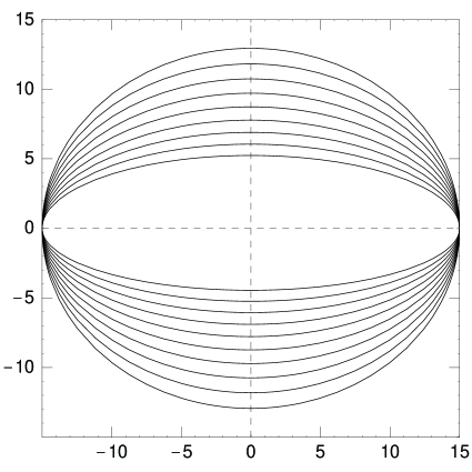
Figure 6: Truncation ellipsoids, each corresponding to a different species. Outer ellipsoid corresponds to the 0.1 $M_{\odot}$ - 1 $M_{\odot}$ mass bin, and then inwards to the species from 1.1 to 2 $M_{\odot}$, by 0.1 $M_{\odot}$ increments.

The corresponding rotation curve is flat, with a circular velocity

$$v_{\rm rot}^{2}(R)=4\pi G\sum_{i}\Lambda_{i}\sqrt{1-e_{i}^{2}}\times\frac{\arcsin e_{i}}{e_{i}}$$ (28)

The surface mass density of species $i$ is

$$\Sigma_{i}(R)=\frac{2\Lambda_{i}\sqrt{1-e_{i}^{2}}}{R}\arctan\left(\frac{\sqrt{R_{\rm max}^{2}-R^{2}}}{R}\right)$$ (29)

With a given set of parameters $(\Lambda_{i},e_{i})$, the local vertical velocity dispersion is defined as

$$\sigma_{W,i}^{2}=\frac{\Phi(R,z)-\Phi(R,0)}{\log\{\rho(R,0)/\rho(R,z)\}}$$ (30)

We define $v_{W,i}$ as the vertical velocity dispersions averaged along $z$, which are more closely related to observable quantities.

$$v_{W,i}(R)=\frac{\int_{-\infty}^{\infty}\rho_{i}(R,z)\sigma_{W,i}(R,z)dz}{\int_{-\infty}^{\infty}\rho_{i}(R,z)dz}$$ (31)

We computed the parameters $\Lambda_{i}$ and $e_{i}$ that realize the following properties:

• The circular velocity is 65 km/s.

• The surface density mass function is given by a Salpeter law (see section 2). As can be seen in (29), this condition can be consistently fulfilled for every radius.

• as in section 2, the average vertical velocity dispersions $v_{W,i}$ vary according to the mass $m_{i}$ as given in (9), from $v_{\rm min}$ to $v_{\rm max}$.

Unlike the disk model, there is an upper limit to the vertical velocity dispersion we can impose. For a one-species model, this limit would be $\sigma_{W}^{\rm max}=V_{c}/\sqrt{2}$, numerically $46\,\mbox{km/s}$, given the chosen rotation velocity. This limit is slightly different for a multi-mass model, but still present. Accordingly, we impose velocity dispersions ranging from $v_{\rm min}=20\,\mbox{km/s}$ for the heavy stars to $v_{\rm max}=45\,\mbox{km/s}$ for the light stars. This is model B-1. For comparison, we also present the results for model B-0 in which all species have a velocity dispersion of 20 km/s. The parameters for model B-1 are shown in table 2.

Table 2: Parameters obtained after convergence for model B-1, i.e. with $v_{\rm max}=45$ km/s.

$$\begin{array}[]{|c|c|c|c|}\hline\cr\hline\cr m[M_{\odot}]&e_{i}&10^{3}\times\Lambda_{i}[M_{\odot}\mbox{pc}^{-1}]&\mbox{v}_{W,i}\mbox{[km/s]}\\ \hline\cr\hline\cr 0.1-1&0.438&70.5&45\\ 1.1&0.663&2.08&39.5\\ 1.2&0.768&2.16&35.2\\ 1.3&0.830&2.22&31.8\\ 1.4&0.869&2.27&29.1\\ 1.5&0.895&2.29&26.8\\ 1.6&0.913&2.30&24.9\\ 1.7&0.927&2.30&23.4\\ 1.8&0.937&2.29&22.1\\ 1.9&0.945&2.26&20.9\\ 2&0.951&2.23&20\\ \hline\cr\hline\cr\end{array}$$

3.2 Microlensing parameters

In a similar way as that explained in section 2.2, it is possible to compute the optical depth and event rate for an ellipsoidal model of the lmc. They are shown in figures 7 and 8 as a function of the distance to the center of the lmc.

Figure 7: Evolution of the optical depth $\tau$ with the distance to the center of the lmc, for the ellipsoidal model and two values of the maximum velocity dispersion: 20 km/s (model B-0) and 45 km/s (model B-1).

Figure 8: Evolution of the event rate $\Gamma$ with the distance to the center of the lmc, for the ellipsoidal model and two values of the maximum velocity dispersion: 20 km/s (model B-0) and 45 km/s (model B-1).

There is a strong decrease of both quantities with the radius, which can be used to test statistically the location of the lenses detected in microlensing experiments. Note that the effect is even more drastic in the ellipsoidal model than in the disk model of the lmc: in the latter, the increased thickness at large radius was compensating the decrease in surface density.

The predicted distributions of event durations, normalized to a maximum value of 1, are shown in figures 9 and 10 at two different distances from the center of the lmc. Since there is no cut-off in the ellipsoidal model, the duration distribution is nearly independent of the maximum velocity dispersion at all radii.

Figure 9: Predicted distribution of event durations for the multi-mass ellipsoidal model at a distance of 1 kpc from the center of the lmc. Plain curve is for model B-1, dashed curve for model B-0.

Figure 10: Predicted distribution of event durations for the multi-mass ellipsoidal model at a distance of 5 kpc from the center of the lmc. Plain curve is for model B-1, dashed curve for model B-0.

4 Discussion and conclusion

We have presented here two models for the lmc, both consistent with the known properties of the Cloud (rotation velocity, surface light density), allowing for a multi-mass stellar population, each associated with a specific velocity dispersion. This correlation between mass and velocity dispersion is justified by the fact that lighter stars are on the average older and had the time to diffuse in velocity space.

These models of the lmc predict an optical depth in agreement with that observed by the macho and the eros collaborations: at a distance of 1 kpc from the lmc center, the disk model yields $\tau_{\mathrm{\mathsc{lmc}}}({\rm disk})\sim 1\times 10^{-7}$ for a velocity dispersion of the lightest and therefore oldest objects of 80 km/s, and the ellipsoidal model yields $\tau_{\mathrm{\mathsc{lmc}}}({\rm ellipsoids})\sim 1.3\times 10^{-7}$ for $v_{\rm max}=45$ km/s.

The optical depth which we have derived results from the interplay of various effects. In the case of the disk model, for instance, Gould’s estimate is only recovered in the thin disk limit. Setting the various stellar velocities at the same value of 80 km/s and pushing the lmc at infinite distance from the Milky Way, we get $\tau_{\mathrm{\mathsc{lmc}}}=1.80\times 10^{-7}$, in agreement with relation (1). If now we assume the same distribution of stellar velocities as in Table 1, i.e. with velocities ranging from 20 to 80 km/s, the optical depth becomes $1.14\times 10^{-7}$. Because the sources have small velocity dispersions, they are fairly concentrated towards the disk, hence a decrease of $\tau_{\mathrm{\mathsc{lmc}}}$ by a factor of $\sim\log 2$. The proeminent effect is actually the presence of the cut-off $z_{\rm max}=\pm 10\;{\rm kpc}$ which we have enforced. At 3 kpc from the center, the optical depth decreases from $1.14\times 10^{-7}$ to $7.57\times 10^{-8}$. At small radii, the surface mass density is large and the disk thickness $a$ is small as compared to $z_{\rm max}$. There, the decrease of $\tau_{\mathrm{\mathsc{lmc}}}$ is less sensitive than towards the outer fringes of the lmc disk, where the cutoff suppression is quite noticeable. Taking furthermore into account the finite distance of 52 kpc to the lmc implies a minor decrease of the optical depth which becomes now $\tau_{\mathrm{\mathsc{lmc}}}(3\;{\rm kpc})=6.63\times 10^{-8}$. Finally, tidal forces tend to stretch the disk, hence a final value of $\tau_{\mathrm{\mathsc{lmc}}}(3\;{\rm kpc})=7.15\times 10^{-8}$.

If the rotation velocity of the lmc $V_{C}$ is set equal to 80 km/s instead of 65, the main impact on our disk model is an increased surface mass density. As the disk becomes thinner, the suppression of the optical depth resulting from the above mentioned cut-off is less sensitive, hence an increased optical depth at large radii. At 3 kpc, the optical depth becomes $9.08\times 10^{-8}$.

In order to model various M/L ratios, we have simply modified the relative contribution of our first stellar bin. That population corresponds to faint stars. Still with $V_{C}=80\;{\rm km/s}$ and at $R=$ 3 kpc, an increase of the M/L ratio by a factor of 2 and 5 respectively leads to 9.43 and $9.67\times 10^{-8}$. The optical depth is thus not sensitive to the precise value of the M/L ratio, insofar as the disk dynamics is dominated by the faint and low-mass species.

Ellipsoids have a lenticular shape. As the radius $R$ increases, their surface mass density drops, and the system becomes thinner towards the edges. Increasing the lmc rotation velocity without changing the velocity dispersion of the various stellar species does not change much the optical depth. Two opposite effects are actually at stake: the first is that the mass densities are larger, the second that the stellar populations are flattened towards the disk. If now the dispersion velocities $\sigma_{W}$ are scaled to the rotation velocity, in order to maintain the shape of the ellipsoids — which depends to first order on the ratio $\sigma_{W}/V_{C}$ — increasing the rotation speed from 65 to 80 km/s results into a significantly larger optical depth. If we set $\sigma_{W}^{\rm max}=55\;{\rm km/s}$ and $V_{C}$ = 80 km/s, the optical depth at 1 and 3 kpc becomes respectively 2.19 and $1.26\times 10^{-7}$. That set of values actually correspond to an lmc mass at 5 kpc of $7\times 10^{9}M_{\odot}$ (Hughes et al. 1991) that increases up to $1.4\times 10^{10}M_{\odot}$ at 10 kpc (Schommer et al. 1992).

Reexamining the status of event MACHO-LMC-9 appears worthwhile. As pointed out in (Bennett, 1996), its measured projected relative velocity was too low both for a Galactic halo event and for self-lensing with a standard lmc disk model. Figure 11 shows the distribution of the expected projected relative velocity for the 80 km/s disk and the 45 km/s ellipsoidal models, along with the measured velocity, for two values of the horizontal velocity dispersion, null or equal to the vertical one – the reality being probably inbetween. The measured value is compatible with an ellipsoidal model, but only compatible with a disk model if the horizontal velocity dispersion is not too high.

Figure 11: Predicted distribution of relative velocity between source and lens, for the ellipsoidal and the disk models, along with the measured value for MACHO-LMC-9 (Bennett et al. 1996). Thin curves: null horizontal velocity dispersion; thick curves: horizontal velocity dispersion equal to the vertical one.

Reconsidering the shape of the lmc and the velocity distributions of its stellar components thus appears to be quite valuable. Two observational projects could yield interesting results in regards to this new perspective, and would help to check the validity of the assumptions made here. Both would be of great consequence for microlensing experiments.

The first of these is the measure of dispersion velocities for RR-Lyrae in the lmc. They indeed form a well-defined sample of very old stars (more than 10 Gyr old). If our model is correct, they should be found to have a higher velocity dispersion than previously measured stars.

The second project is actually a pure extension to the present microlensing experiments. As evidenced in this paper, self-lensing in the lmc can be tested quite accurately with the spatial evolution of the microlensing parameters such as optical depth and event rate. Searching for microlensing events on as large an area as possible over the lmc would be a very powerful tool to discriminate between halo and lmc deflectors, because of the strong decrease of $\tau_{\mathrm{\mathsc{lmc}}}$ and $\Gamma_{\mathrm{\mathsc{lmc}}}$ with the distance to the center of the lmc in the case of self-lensing. In addition to the implications such observations would have on the galactic dark matter issue, they would be of great use for a better understanding of the structure of the lmc, the nearest galaxy to the Milky Way. Furthermore, as shown in (Gould 1998), monitoring as large an area as possible on the lmc, using the same exposure time on inner and outer fields, optimizes the total number of expected events, even for Galactic halo lensing. Such a strategy would be even more productive if associated with a real-time trigger and a high precision follow-up strategy, yielding high quality microlensing light-curves on which testing for parallax effect would provide information on the location of the lenses.