Simulations of small-scale explosive events on the Sun

Abstract

Small-scale explosive events or microflares occur throughout the chromospheric network of the Sun. They are seen as sudden bursts of highly Doppler shifted spectral lines of ions formed at temperatures in the range $2\times 10^{4}-5\times 10^{5}$ K. They tend to occur near regions of cancelling photospheric magnetic fields and are thought to be directly associated with magnetic field reconnection. Recent observations have revealed that they have a bi-directional jet structure reminiscent of Petschek reconnection. In this paper compressible MHD simulations of the evolution of a current sheet to a steady Petschek, jet-like configuration are computed using the Versatile Advection Code. We obtain velocity profiles that can be compared with recent ultraviolet line profile observations. By choosing initial conditions representative of magnetic loops in the solar corona and chromosphere, it is possible to explain the fact that jets flowing outward into the corona are more extended and appear before jets flowing towards the chromosphere. This model can reproduce the high Doppler shifted components of the line profiles but the brightening at low velocities, near the centre of the bi-directional jet, cannot be explained by this simple MHD model.

1 Introduction

The quiet Sun chromospheric network is teeming with tens of thousands of small-scale explosions. They have a typical lifetime of 60 s, sizes of 2000 km and flow velocities of about 100 km s^-1. They were discovered in high resolution ultraviolet spectra of the Sun (Brueckner and Bartoe, 1983; Dere, Bartoe and Brueckner, 1989). They appear as small sites with large red and/or blue Doppler shifted emission lines of species which are formed at electron temperatures in the range $5\times 10^{4}-5\times 10^{5}$ K. Recent observations have revealed several examples where the spatial and temporal evolution of the line profiles clearly indicate bi-directional flows (Innes et al, 1997; Wilhelm et al., 1998).

Several features suggest that the flows are quasi-steady and there is continual heat input at a local site at the centre of the event rather than a real explosion. For example, the position with the brightest emission, which also looks like the central position of the bi-directional jet, moves with a velocity less than 5 km s^-1 transverse to the line-of-sight (Dere, 1994). Also the lifetime of the events, typically 60 s, is considerably longer than the cooling time of the plasma, about 5 s (assuming a temperature $10^{5}$ K and density $10^{10}$ cm^-3 (Dere et al., 1991)).

Further clues to the flow come from comparing line profiles observed at the centre of the Sun’s disk and towards the limb of the disk. At disk centre the profiles tend to have short, bright red-shifted components and more extended, fainter blue-shifted components. Also the blue wing tends to emerge first. The profiles from events occurring towards the solar limb have more similar red and blue components (Innes et. al, 1997). So it seems as though the extent of the flow and its properties depend strongly on the conditions surrounding the flow.

There are several suggestions for the underlying process triggering these events. The first, by Dere et al. (1991) and supported by Priest (1998), is that they are due to magnetic reconnection between network magnetic fields and emerging loops. In this case the observed bi-directional flows would be reconnection jets. Another idea is that they are chromospheric evaporation as a result of coronal microflares (Krucker et al., 1997). Yet another idea that would also explain the observed pattern of red-blue Doppler shifts, is that they are swirling funnels of gas or tornadoes (Pike and Mason, 1998). It should be possible to use available high resolution ultraviolet spectroscopic observations to judge these suggestions. To date there have been no theoretical models capable of predicting emission spectra from any of these scenarios.

In this paper we make a first attempt at computing the behaviour of different temperature emission lines from a Petschek-like reconnection scenario (Petschek 1964). The Petschek solution is a special case of fast steady state reconnection (Priest and Forbes, 1986; Priest and Lee, 1990) in which reconnection occurs at a small localized X-type neutral point along a narrow current sheet. As described by Petschek, material flows into the reconnection point and is ejected with the Alfvén velocity in both directions along the neutral sheet. Although there have been several numerical simulations of this type of 2-D reconnection (e.g. Sato and Hyashi, 1979; Biskamp, 1986; Yan, Lee and Priest, 1991; Jin, Inhester and Innes, 1996) the conditions in the upper chromosphere/lower transition zone are rather different to those dealt with in other simulations. This region is characterized by small, loop-like structures with typical temperatures of a few times $10^{4}$ K and densities about $10^{10}$ cm^-3 (Dere et al., 1991; Wilhelm et al., 1998). Anti-parallel magnetic fields may be driven together by, for example, loop footpoint motion, rising loops or by the buffeting effect of neighbouring gas motions.

We are not trying to simulate any specific set of observations but to obtain a realistic feel for the characteristic flow and spectrum under different conditions. In section 2 the simulation models, the boundary and initial conditions are described. In the next section the basic features of the current sheet evolution, the line profiles and their temperature dependence are shown. Finally the strengths and weaknesses of the models are discussed.

2 Simulation Model

The evolution is described by the compressible magnetohydrodynamic (MHD) equations in the following form:

$${\frac{\partial\rho}{\partial t}}+\nabla\cdot({\vec{v}}\rho) = 0$$

$${\frac{\partial\rho{\vec{v}}}{\partial t}}+\nabla\cdot({\vec{v}}\rho{\vec{v}}-{\vec{B}}{\vec{B}})+\nabla p_{\mathrm{tot}} = 0$$

$${\frac{\partial E}{\partial t}}+\nabla\cdot({\vec{v}}E+{\vec{v}}{p_{\mathrm{tot}}}-{\vec{B}}{\vec{B}}\cdot{\vec{v}}) = \nabla\cdot\left({\vec{B}}\times\eta{\vec{J}}\right)-{Q_{\mathrm{rad}}}$$

$${\frac{\partial{\vec{B}}}{\partial t}}+\nabla\cdot({\vec{v}}{\vec{B}}-{\vec{B}}{\vec{v}}) = -\nabla\times\left(\eta{\vec{J}}\right)$$ (1)

where $\rho$, $\rho{\vec{v}}$, $E$ and ${\vec{B}}$ are the density, momentum density, total energy density and magnetic field, $\eta$ is the resistivity coefficient and ${\vec{J}}=\nabla\times{\vec{B}}$ is the current density. The magnetic units are chosen so that the magnetic permeability (or the $4\pi$ factor of cgs) does not appear in the equations. The total pressure ${{p_{\mathrm{tot}}}}=p+{\vec{B}}^{2}/2$. The thermal pressure $p$ is related to the total energy density $E$ by

$$p=\left(\gamma-1\right)\left(E-\rho{\vec{v}}^{2}/2-{\vec{B}}^{2}/2\right),$$ (2)

for an ideal gas with adiabatic index $\gamma$. In these computations $\gamma=5/3$. The temperature units are chosen such that $T=p/\rho$. The radiative losses are represented by ${Q_{\mathrm{rad}}}$ and the expression used is that given in Rosner, Tucker and Viana (1978). In the solar transition there are heat sources, for example thermal conduction, wave or photon heating, that prevent the gas cooling below a few times $10^{4}$ K. These sources are ill-defined and in our simulations we simply decrease the radiative losses to zero at $2\times 10^{4}$ K. This means that if the initial temperatures are above $2\times 10^{4}$ K, the initial state is not in thermal equilibrium. In the simulations discussed here the timescale for cooling from the initial configuration is long compared to the simulation timescale.

The MHD equations are solved using a high resolution shock capturing Total Variation Diminishing Lax-Friedrichs scheme. This is one of the schemes available in the Versatile Advection Code software package (Tóth 1996, 1997). This scheme has been well tested and proved accurate and stable in the simulation of steady 2-D reconnection (Tóth, Keppens and Botchev, 1998). The equations are solved on a non-uniform 2-D Cartesian grid. Due to the symmetry of the problem, only one quarter of the reconnection region is represented. The computational domain $x\in[0,2]$ and $y\in[0,8]$ is resolved by a $150\times 150$ grid. The cell size increases logarithmically from $\Delta x=0.0005$ at $x=0$ to $\Delta x=0.1$ at $x=2$. This gives good resolution at the neutral point, while the coarser grid at the boundaries damps the outward travelling waves without reflection.

According to the symmetry of the problem, the boundary conditions are symmetric for $\rho,\ \rho v_{x},\ E$, and $B_{y}$ and anti-symmetric for $\rho v_{y}$ and $B_{x}$ along the $x$-axis, while along the $y$-axis the variables $\rho,\ \rho v_{y},\ E$, and $B_{x}$ are symmetric, and $\rho v_{x}$ and $B_{y}$ are anti-symmetric. At the top boundary, all physical quantities are extrapolated into the boundary with zero gradient. At the right, we fix $\rho,\ \rho v_{y}$ and $B_{y}$ to their initial values, while the inflow mass flux $\rho v_{x}$ is extrapolated from the outer cell on each row so that the inflow speed is determined by the reconnection rate at the current sheet. Likewise, the initially zero $B_{x}$ is extrapolated continuously from the last cell row so that the field lines can bend in response to the inflow.

The initial configuration of the magnetic field has a current sheet at $x=0$ with a characteristic width $L$. The field is parallel to the $y$-axis and varies only along the $x$-axis according to

$$B_{y}(x)={\mathrm{tanh}}(x/L).$$ (3)

In our normalization $B_{y}=1$ for $x\gg 1$. We also take the density to be unity at the boundary, thus the Alfvén speed $B/\sqrt{\rho}$ is also unity.

The initial magneto-hydrostatic equilibrium is maintained by the total pressure $p_{\mathrm{tot}}$ being constant throughout. Consequently, the initial distribution of thermal gas pressure $p$ is

$$p(x)={p_{\mathrm{tot}}}-B^{2}_{y}(x)/2=p_{\infty}+\frac{1}{2}\mathrm{sech}^{2}(x/L)$$ (4)

where $p_{\infty}$ is the thermal pressure at $x\gg L$. The plasma beta at large $x$ is $\beta=2p/{\vec{B}}^{2}=2p_{\infty}$. The initial magnetic and gas pressure across the current sheet are plotted in Figure 1.

Given the initial magnetic and gas pressure distribution described above, there is still a free choice of temperature and density distributions. This allows us to apply this simple current sheet reconnection model to a range of initial conditions representing different parts of the solar atmosphere. For this first study, the two simplest initial density/temperature configurations are considered: a uniform temperature solution, $T=p_{\infty}$, and a uniform density solution, $\rho=1$. Then the density and temperature are given by $\rho(x)=p(x)/T$ and $T(x)=p(x)/\rho$, respectively. The enhancement factor of the density/temperature is $1+1/\beta$ at the centre of the current sheet ($x=0$) relative to the value outside ($x>>L$). Thus along the centre of the current sheet, the density is $1+1/\beta$ in the uniform temperature case ($T=\beta/2$) and the temperature is 1/2 in the uniform density case ($\rho=1$).

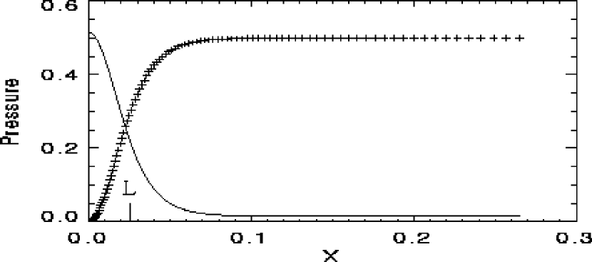
Figure 1: The initial gas and magnetic (+++) pressure across the current sheet with characteristic width $L=0.025$. The crosses are placed at the centre of each computational cell.

In the uniform density case $\beta$ determines the strength of the shock at the jet head. The jet speed approximately equals the Alfvén speed at large $x$, which is unity, while the sound speed in the neutral sheet ahead of the jet is $\sqrt{\gamma p/\rho}=\sqrt{\gamma(1+\beta)/2}$. If $\beta>2/\gamma-1=0.2$, the jet is subsonic. In the final steady solution $\beta$ determines the compression and opening angle of the jet (Petschek, 1964). In our simulations we used $\beta=0.03$.

The small central region has an enhanced resistivity that decreases exponentially from the centre of symmetry by

$$\eta({\vec{x}})=\eta_{0}\exp\left[-(x/\ell_{x})^{2}-(y/\ell_{y})^{2}\right],$$ (5)

where the constants $\eta_{0}=0.0005$ and $\ell_{x}=\ell_{y}=0.025$ determine the resistivity at the origin and the width of the resistivity profile in the $x$ and $y$ directions.

3 Results

3.1 EVOLUTION TO STEADY STATE

We start from an equilibrium configuration with two regions of oppositely directed field lines. The localized anomalous resistivity initiates the onset of the reconnection process between the two regions, and an X-type neutral point forms. The anomalous resistivity is required to break the initial symmetry and to maintain the position of the X-point. In the small region around the X-point, the current density is high and plasma is accelerated out along the current sheet (Yan, Yee and Priest, 1992). In these MHD simulations we do not expect the detailed evolution in the vicinity of the X-point to be well modelled. Our aim is to obtain the basic large-scale flow structure and in particular the heating, compression and acceleration behind the slow and fast magnetoacoustic shocks.

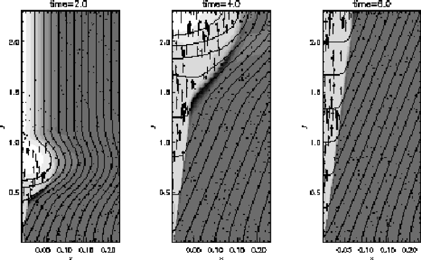
Figure 2: Evolution of uniform density current sheet. Shown are the temperature (dark tones correspond to low temperature), velocity vectors, and magnetic field lines. Only a small part of the full computational domain is plotted and the $x$ direction is strongly stretched.

Outside the diffusion region, the plasma flows out in narrow jets along the current sheet. The evolution for a low beta, $\beta=0.03$, and uniform initial density is shown in Figure 2. This shows the evolution of the temperature, magnetic field and the velocity vectors after the initial build up of the flow around the X-point. The flow at the jet head is supermagnetosonic and there is a fast magnetoacoustic shock. It shows up as a broad high temperature region with enhanced $B_{x}$. This fast shock was not seen in the compressible MHD computations of Sato and Hayashi (1979) because they used $\beta=1$ so the sound speed along the current sheet was greater than the Alfvén speed outside. Once the shock has propagated off the grid the final system reaches a steady state. The gas in the jet moves at the Alfvén speed along the current sheet. There is a slow magnetoacoustic or switch-off shock along the boundary of the jet that makes an angle $\alpha=0.025\approx\eta_{o}^{1/2}$. In the inflowing plasma, the magnetic field decreases from the boundary at $x\gg 1$ towards the jet while the gas pressure remains almost unchanged. This is essentially the steady state Petschek solution (Petschek, 1964). Other simulations made with different resistivity show that the opening angle of the jet depends on the size of the resistivity and the width of the resistivity function (Yan, Lee and Priest, 1992). The structure of the fast magnetoacoustic shock depends on the conditions in front of the shock. Forbes (1986) has studied the structure of stationary fast magnetosonic shocks at the head of reconnection jets directed towards closed magnetic loops tied to the photosphere.

3.2 COMPARISON WITH OBSERVATIONS OF EXPLOSIVE EVENTS

The chromosphere-corona transition region of the solar atmosphere (heights less than 4000 km) is dominated by two temperature regimes. The gas closest to the solar surface has a temperature around $10^{4}$ K and the coronal gas has a temperature around $10^{6}$ K. Gas at intermediate temperatures cools rapidly and the line emission from ions formed at these temperatures is very variable and seems to be coming from small dynamic sites. Explosive events are just one well observed example of this variability.

The main evidence that explosive events are bi-directional jets comes from a study of their ultraviolet emission line profiles. Innes et al. (1997) show examples where the line-shifts, corresponding to velocities of about 100 km s^-1, change from blue to red within about $2000$ km. This is what one would expect if looking at some small angle to the flow axis of a bi-directional jet. Innes et al. also show cases where the length of the region with high line-shifts increases during the event lifetime suggesting propagation of jets into the surrounding material. The blue and red streams often appear to be asymmetric in the sense that, particularly at disk centre, the region with blue-shifted emission is more extended and appears before the region with red-shifted emission.

3.2.1 Structure

In order to model the explosive events the absolute lengths, density and velocity units are chosen to be $1000\,$km, $5\times 10^{9}\,$cm^-3 and $141\,$km s^-1 respectively. Then the time unit is $7\,$s and the temperature unit is $\frac{m}{2k}v^{2}_{unit}=1.44\times 10^{6}\,$K, where $m=2\times 10^{-24}\,$g is the mean mass of atoms, $k$ is Boltzmann’s constant and $v_{unit}$ is the velocity unit. This gives a temperature about $2\times 10^{4}$ K in the high field region of the current sheet. The cooling time for shock heated inflow gas is about 4 s. The uniform density initial condition has a density of $5\times 10^{9}\,$cm^-3 throughout, a temperature of $7\times 10^{5}$ K along the neutral sheet and $2\times 10^{4}$ K at the inflow boundary. The other case, the uniform temperature initial condition, has a temperature of $2\times 10^{4}$ K throughout, a density of $1.7\times 10^{11}$ cm^-3 along the neutral sheet and $5\times 10^{9}$ cm^-3 at the inflow boundary. These two cases can be thought of as representing magnetic loops in the corona and magnetic loops in the chromosphere.

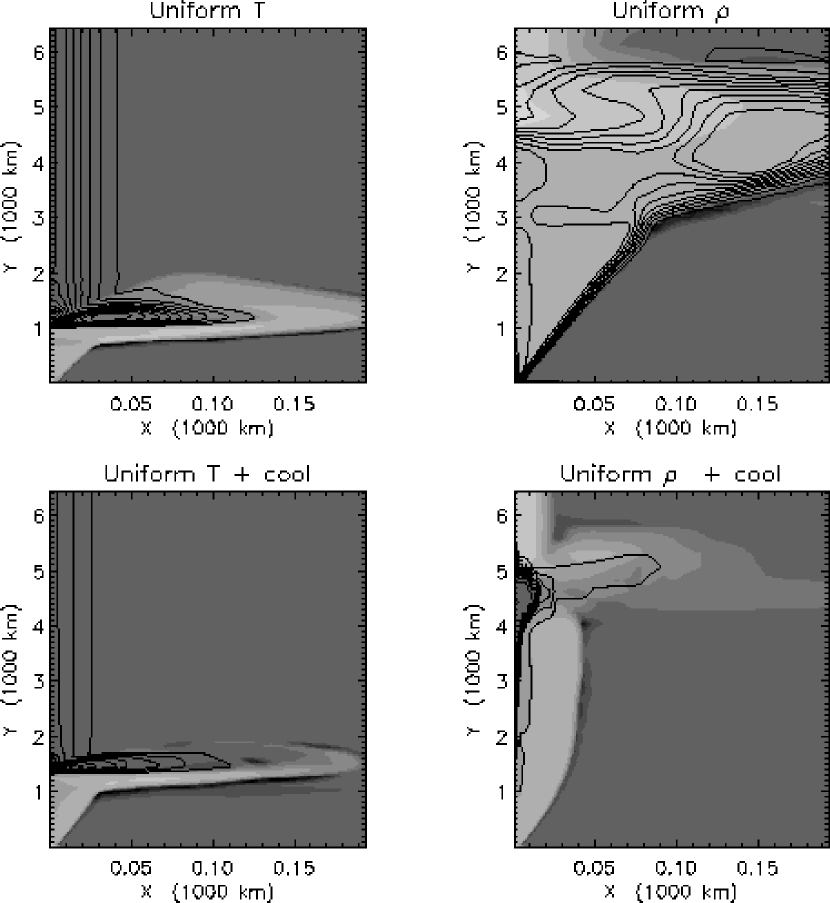
Figure 3: The temperature and density (contours) structure of the reconnection jet at time=50 s for the uniform temperature and density initial conditions, without and with radiative cooling.

The temperature and density structure for the two cases with and without radiative cooling are shown at a time 50 s in Figure 3. Here the different evolution scenarios are well illustrated. The jet moves out at a speed that depends on the square root of the neutral sheet density. Thus the jet length is about 6 times more in the uniform density case. A natural consequence of this model is that jets into the hot tenuous corona will be longer and appear before jets into the much denser chromosphere. This may explain why observations made at disk centre often show more extended blue-shifted than red-shifted emission and why the blue-shifted emission often occurs first. The jet itself on the other hand has the same opening angle, velocity and density in both cases.

Radiative cooling considerably changes the structure of the jet. As shown for the jet from the uniform density initial condition (right hand panels of Figure 3), the jet and its head are much narrower. The fast shock at the jet head is confined to the narrow neutral sheet region and the postshock material cools quickly. In the case with uniform temperature initially (left hand panels) the narrowing of the jet is not obvious because after 50 s the jet length is hardly longer than the cooling length. The temperature and density structure of the cooling jet and their relationship to the jet flow and magnetic field are shown in Figure 4. As in the case without radiative losses, the slow magnetoacoustic shocks accelerate and heat plasma along the boundary of the jet. Now the gas cools as it flows along the jet. The structure along a streamline is similar to models of 1-D radiative shocks (e.g. Cox, 1972). Along the central axis is a cold jet core. As we shall see, this shows up as a high velocity, low temperature component in the line profiles.

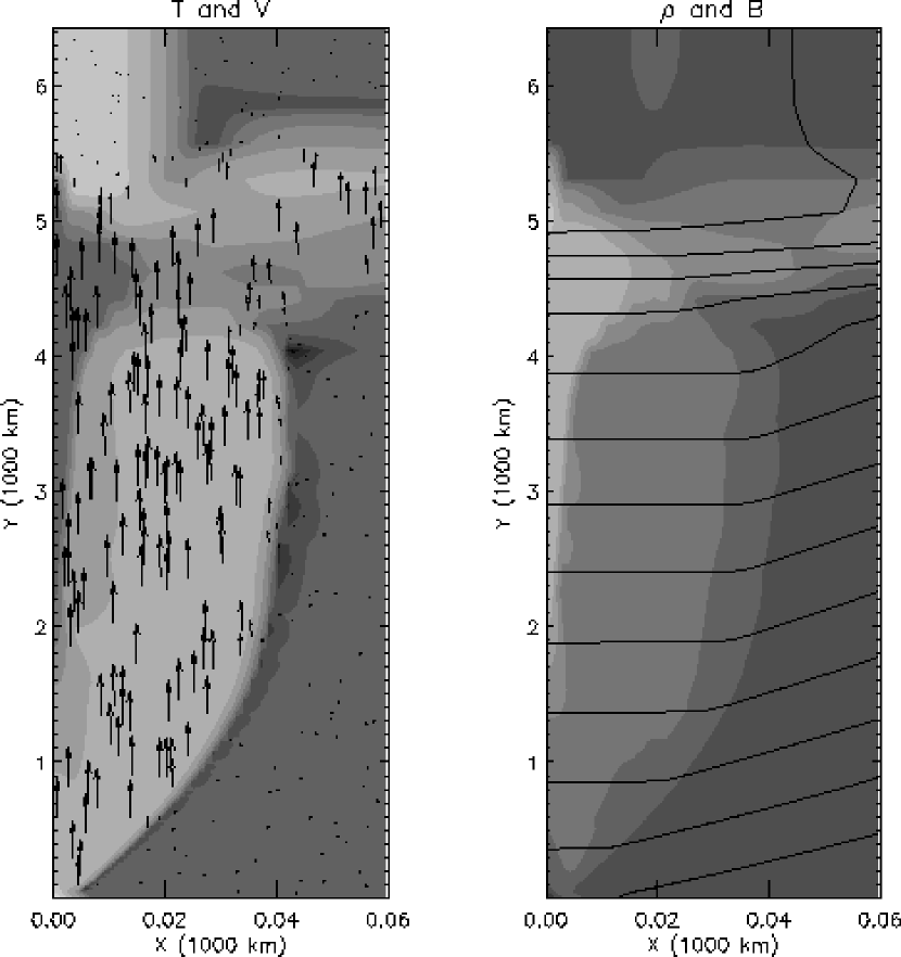
Figure 4: The jet structure when radiative cooling is included in the solution starting from uniform density. On the left is temperature and velocity and on the right density and magnetic field.

3.2.2 Line profiles

As we have seen there are three basic regions in the jet structure. There is the jet source or X-point where magnetic diffusion dominates. Coming out of the X-point are the reconnection jets. These are bounded by standing magnetoacoustic shocks and may have cold high velocity cores. At the head of the jet is a fast magnetoacoustic shock that moves outwards from the central source at a speed depending on the ram pressure of the jet and the density in the neutral sheet. These three regions have different spectral characteristics and under favourable observing conditions it should be possible to spatially resolve the regions.

The intensity of an emission line formed over a restricted temperature range, $T_{\max}$ to $T_{\min}$, is the integral of the emissivity along the line-of-sight,

$$I=\int\int_{T_{\min}}^{T_{\max}}\rho^{2}{\epsilon}(T)dTdz$$ (6)

where $dz$ is the line-of-sight path increment and the temperature dependence of the line emission is represented by the function ${\epsilon}(T)$. In our approximation, we have assumed that ${\epsilon}(T)$ is a simple function defined as

$${\epsilon}(T)\equiv\left\{\begin{array}[]{ll}1&\mbox{if $T_{\min}<T<T_{\max}$}\\ 0&\mbox{otherwise.}\end{array}\right.$$ (7)

The profiles, shown in Figures 6–8, are obtained by computing the total intensity of line emission from gas with a line-of-sight velocity $v$. Thus the intensity in a given velocity interval $v$ to $v+dv$ is

$$I_{[v,v+dv]}=\sum_{i}\rho_{i}^{2}{\epsilon}_{i}dx_{i}dy_{i}$$ (8)

where the summation is over each cell, $i$, in the appropriate region of the computational domain with line-of-sight velocity between $v$ and $v+dv$. We used velocity bins of size $dv=1\,$km s^-1.

The profiles are given for three temperature regimes $<2\times 10^{4}\,$K, $8\times 10^{4}-2\times 10^{5}\,$K and $>5\times 10^{5}\,$K. These ranges have been chosen because they outline the explosive event distribution in temperature as inferred from the number of events seen in various emission lines. There are many events seen in lines formed in the middle temperature range, a few above $5\times 10^{5}$ K and almost none below $2\times 10^{4}$ K.

As far as possible we would like to compare the numerical models directly to observations therefore we have computed line profiles from sections of the models with a scaled length of 2000 km. This is close to the spatial resolution of the spectrometer SUMER (Wilhelm et al., 1995, 1997; Lemaire et al., 1997), the instrument on board SOHO, with which it was possible to spatially resolve and observe the evolution of explosive events (Innes et al., 1997). Solutions with different temperature/density initial conditions differ only in the fast shock structure at the jet head and the propagation speed of the jet but not in the jet structure itself. Therefore we use the solution from the uniform density initial condition to show the evolution of the jet. In this simulation the jet moves a distance of 5000 km in 50 s. The different regions of such a jet fall conveniently into 2000 km spatial sections. For the other initial condition, only the profiles from the full jet structure are shown.

The profiles from the uniform density evolution are displayed in Figures 6 and 7. These figures are organized so that each row corresponds to a different temperature, each column to a different section of the grid and different plot line styles distinguish profiles at different times. The spatial sections are marked on Figure 5 and labelled ‘jet source’, ‘jet’ and ‘jet head’. These labels describe the structure at 50 s. At earlier (or later) times different regions of the jet fill these sections of the computational grid. For example at 30 s the jet head is in the ‘jet’ section. The ‘jet source’ region covers both the up- and downward flowing jet. For this region the profiles are computed after reflecting the structure from the lower 1000 km across the $x$-axis. This makes it easier to see the relative intensities in the high and zero velocity components at the centre of the bi-directional jet. All profiles are shown for a viewing angle of $45$ degrees. Thus a jet flowing along the axis at the Alfvén speed at $x>>L$ has a line-of-sight velocity 100 km s^-1.

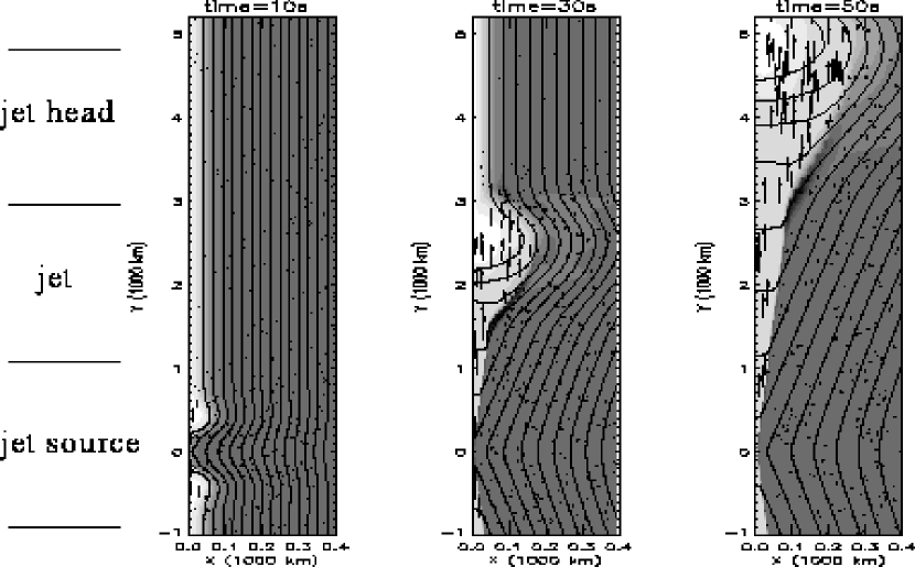
Figure 5: The uniform temperature jet structure at the three times where line profiles are calculated. The spatial sections over which the profiles have been integrated are marked. The names are relevant for the structure at time 50 s.

High velocity emission is seen in the middle and high temperature range for the evolution without radiative cooling. At middle temperatures both the jet and the head emit. In this simulation and at this viewing angle (45 degrees), the profiles appear broad. The velocity of the emission from the jet head is smaller than from the jet because the head emission is coming from the sides of the jet head where the flow velocity is less than the on-axis flow. The shock at the jet head is about a factor $2$ brighter than the jet. This ratio depends on the strength of the fast shock at the jet head. For higher values of $\beta$ the shock and the jet emission are weaker. The high temperature emission is coming from the central front of the fast shock and only the jet head, not the jet itself shows up in hot lines. At $T<2\times 10^{4}$ K there is no high velocity plasma. The emission is coming from a thin region just upstream of the slow mode shock.

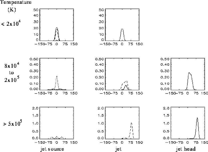
Figure 6: Line profiles (relative intensity vs. velocity in km s^-1) from the uniform density initial condition. Each row shows line profiles at the temperatures given on the left, from the three sections labelled on the bottom and marked in Figure 5. The different line profiles correspond to different times. t = 10 s (dotted), t = 30 s (dashed) and t = 50 s (solid). The line-of-sight is 45 degrees to the jet axis.

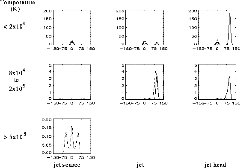
Figure 7: Line profiles from the uniform density condition with cooling. The lay-out of the figure is as described in Figure 6.

As shown in Figure 7, when radiative cooling is included in the computations, the high temperature emission disappears and cold high velocity profiles are obtained due to the formation of the cold jet core. As the head moves out the intensity of the cold temperature line increases (c.f. right panel of the top row). In the middle temperature range high velocity emission is produced along the jet and near the centre of the fast shock. In the example illustrated here, there is also a weak lower velocity component coming from flows along the outer edge of the jet head. As in the simulation without radiative cooling, the relative strength of the emission from the jet head and jet depends on the flow structure at the jet head. This in turn depends strongly on initial conditions.

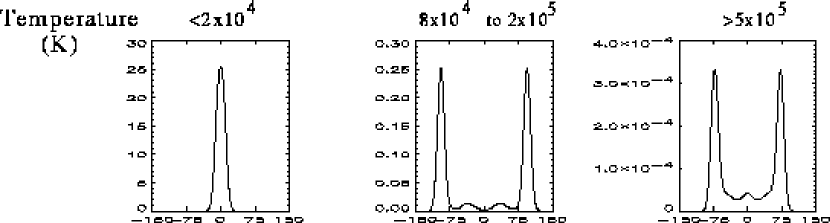
Figure 8: Line profiles at three different temperatures at $t=50\,$s, from the current sheet starting with a uniform temperature. This shows the total jet profiles from the structure reflected across the $x$-axis.

The final set of profiles, given in Figure 8, are from the uniform temperature initial condition with radiative losses at $t=50\,$s. At this time, as can be seen in Figure 3, the jet head has only moved 1 length unit (1000 km) so the profiles shown here are the profiles from the full structure after it has been reflected across the $x$-axis. The profiles from the equivalent structure in the evolution of the uniform density current sheet are the dotted lines ($t=10\,$s) in Figures 6 and 7.

The low temperature profiles are dominated by emission from the plasma in the high magnetic field region of the current sheet. The jet emission produces only very low intensity wings on the original zero velocity profile. At middle temperatures the high velocity components are strong and have a double component structure. Again the highest velocities are coming from the jet and the lower velocity component from the jet head. The high temperature brightening is very weak. The emission is mostly coming from the gas on-axis just behind the fast shock. The velocity is slightly less than the jet velocity.

4 Discussion

Although these models are gross simplifications of the solar structure they illustrate a few basic features of the emission from reconnection jets. (1) High velocity components in lines formed at temperatures $\approx~{}10^{5}$ K, are emitted from the jet irrespective of initial conditions. (2) The jet length depends on the ram pressure (which is controlled by the reconnection rate) and the density in front of the jet. (3) There is no brightening in zero velocity emission either along the jet or at the reconnection point. (4) Due to radiative cooling the jets have cold cores and this may produce high Doppler shifts in cold lines. (5) Multiple components or broad line profiles may be obtained in lines formed $\approx~{}10^{5}$ K due to different flow velocities at the jet head and along the jet. Features such as the ratio of the line intensity in the jet head and jet are very dependent on initial conditions and cannot be used as a test for the model. Features (1), (2) and (5) are consistent with observations but (3) and (4) are not.

High velocity emission in cold lines, feature (4), may actually be present in the data but weak compared to the background because the filling factor of the jets is very small. In a $10^{9}$ km³ volume the jet would occupy at most $10^{-4}$ of the space. By careful analysis of SUMER data, it should be possible to obtain upper limits to the amount of cold high velocity material and thus obtain a better assessment of the model.

The other failing is maybe more serious but even so there is no definitive reason to reject the basic model. The diffusion region is not well represented by the 2-D MHD simulations. In 3-D simulations the diffusion region breaks up into many small high density islands (Otto, 1998). These would most likely generate bright broad profiles in lines formed around $10^{5}$ K. Also particle simulations have shown that electrons are easily trapped in the diffusion region where they are rapidly accelerated (Büchner and Kuska, 1997). These high energy electrons may heat the surrounding low velocity inflowing plasma.

The main success of the model is that due to the presence of slow magnetoacoustic shocks along the jets’ boundary, it is able to explain the almost stationary red and blue shifted emission at high (supersonic) velocities in lines with formation temperatures around $10^{5}$ K for a period much longer than the cooling time of the gas.