Predictions for The Very Early Afterglow and The Optical Flash

Abstract

According to the internal-external shocks model for $\gamma$-ray bursts (GRBs), the GRB is produced by internal shocks within a relativistic flow while the afterglow is produced by external shocks with the ISM. We explore the early afterglow emission. For short GRBs the peak of the afterglow will be delayed, typically, by few dozens of seconds after the burst. For long GRBs the early afterglow emission will overlap the GRB signal. We calculate the expected spectrum and the light curves of the early afterglow in the optical, X-ray and $\gamma$-ray bands. These characteristics provide a way to discriminate between late internal shocks emission (part of the GRB) and the early afterglow signal. If such a delayed emission, with the characteristics of the early afterglow, will be detected it can be used both to prove the internal shock scenario as producing the GRB, as well as to measure the initial Lorentz factor of the relativistic flow. The reverse shock, at its peak, contains energy which is comparable to that of the GRB itself, but has a much lower temperature than that of the forward shock so it radiates at considerably lower frequencies. The reverse shock dominates the early optical emission, and an optical flash brighter than 15th magnitude, is expected together with the forward shock peak at x-rays or $\gamma$-rays. If this optical flash is not observed, strong limitations can be put on the baryonic contents of the relativistic shell deriving the GRBs, leading to a magnetically dominated energy density.

1 Introduction

The original fireball model was invoked to explain the Gamma-Ray Bursts (GRBs) phenomena. Extreme relativistic motion, with Lorentz factor $\gamma>100$ is necessary to avoid the attenuation of hard $\gamma$-rays due to pair production. Such extreme relativistic bulk motion is not seen anywhere else in astrophysics. This makes the GRBs a unique and extreme phenomena. Within the fireball model the observed GRB and the subsequent afterglow all emerge from shocked regions in which the relativistic flow is slowed down. We don’t see directly the “inner engine” which is the source of the whole phenomenon. It is therefore, of the utmost importance to obtain as much information as possible on the nature of this flow as this would provide us with some of the best clue on what is producing GRBs.

The afterglow, that was discovered more than a year ago, has revolutionized GRB Astronomy. It proved the cosmological origin of the bursts. The observations, which fit the fireball theory fairly well are considered as a confirmation of the fireball model. According to this model the afterglow is produced by synchrotron radiation produced when the fireball decelerates as it collides with the surrounding medium.

However, the current afterglow observations, which detect radiation from several hours after the burst onwards, do not provide a verification of the initial extreme relativistic motion. Several hours after the burst the Lorentz factor is less than $\sim 10$. Furthermore, at this stage it is independent of the initial Lorentz factor. These observation do not provide any information on the initial extreme conditions which are believed to produce the burst itself.

It was recently shown (Sari & Piran, 1997, Fenimore, Madras & Nayakshin 1996) that the burst itself cannot be efficiently produced by external shocks, and internal shocks must occur. This has lead to the internal-external scenario. The GRB is produced by internal shocks while the afterglow is produced by external shocks. Additionally there are some observational evidence in favor of the internal-external picture. First, the fact that afterglows are not scaled directly to the GRB suggest that the two are not produced by the same phenomenon. Second, while most GRBs show very irregular time structure and are highly variable all afterglow observed so far show smooth power law decay with minimal or no variability. Still this evidence is so far somewhat inconclusive. In view of the importance of its implications we should search for an additional proof. We suggest here that observation of the early afterglow could provide us with a verification of this picture.

In the internal shocks GRB the time scale of the bursts and its overall temporal structure follow to a large extend the temporal behavior of the source which generates the relativistic flow and powers the GRB (Kobayashi, Piran & Sari, 1997). A fast shell, with a Lorentz factor $>2\gamma$, will catch up with a slower shell of Lorentz factor $\gamma$, that was emitted $\delta t$ earlier, at a radius of $R\sim 2\gamma^{2}c\delta t$. The observed time for this collision will be therefore $R/2\gamma^{2}\sim\delta t$. The fact that the Lorentz factor cancels out shows that the observed temporal structure of the burst cannot provide any information on the initial Lorentz factor in which the shell was injected.

The initial Lorentz factor is a crucial ingredient for constraining models of the source itself. The initial Lorentz factor specifies how “clean” the fireball is as the baryonic load is $M=E/\gamma_{0}$. A very high Lorentz factor would indicate a very low baryonic load which would indicate some sort of electromagnetic acceleration or even Poynting flux flow. More moderate Lorentz factors could more easily allow for the usual hydrodynamic models. The previous discussion shows that we cannot infer on the initial Lorentz facer from the observed temporal structure in GRBs. Unfortunately the spectrum of the GRBs can provide only a lower limit to this this Lorentz factor. This lower limit of $\sim 100$ is given by the appearance of high energy photons, which would have produces pairs is the Lorentz factor was low (Fenimore, Epstein, & Ho, 1993; Woods & Loeb, 1995; Piran, 1997). In the internal shock scenario the observed spectrum depends on the Lorentz factor only via the blue shift. However, the frequency in the local frame is highly unknown since it depends on many poorly known parameters such as the fraction of energy given to the electrons, the magnetic field and the relative Lorentz factor between shells. Therefore the spectrum can not teach us much about the initial Lorentz factor.

Furthermore, the basic mechanism by which the burst is produced, internal or external shocks, must be understood before a reliable source model can be given. External shocks could be produced by a single short explosion. Internal shocks require, however, a long and highly variable wind. The inner engine should operate for a long time - as long as the duration of the burst. We must know whether the source operates for a millisecond or for tens or even hundreds or thousand of seconds.

Mochkovitch, Maiti & Marques (1995) and Kobayashi, Piran & Sari, (1997) have shown that only a fraction of the total energy of the relativistic flow could be radiated away by the internal shocks. This means that an ample amount of energy is left in the flow and a significant fraction of it can be emitted by the early afterglow.

GRBs are among the most luminous objects in the universe. They produce a huge fluence, mostly in $\gamma$-rays. If this fluence was released optically, a flash of 5th magnitude would have been produced. A magnitude of 5 is by far stronger than current observational upper limits on early optical emission. In fact, even a small fraction of this will be easily observed. It is therefore of importance to calculate any residual emission in the optical band (Sari & Piran 1999).

We explore in this paper the expected prompt (early afterglow) multi wavelength signal. We show that this initial afterglow signal could, when it be measured, provide us with information on the initial Lorentz factor and at least indirectly hint on the nature of the relativistic flow. These could provide some important clues on the nature of the “inner engine” that powers GRBs. The physical model of the afterglow is synchrotron emission from relativistic electrons that are being continuously accelerated by an ongoing shock with the surrounding medium. We consider both the emission due to the hot shocked surrounding medium and from the reverse shock that is propagating into the shell. The spectral characteristics of the synchrotron emission process are unique while the light curve depends on the hydrodynamic evolution, which is more model dependent. We begin, therefore (in section 2) exploring the broad band spectrum due to the forward shock. Then we turn (in section 3) to discuss the possible light curves in several frequency regimes. In section 4 we show how future observations of the early afterglow can be used to estimate the initial Lorentz factor. We show that a detection of a delay between the GRB and its afterglow as well as observation of the characteristic frequency in the early afterglow can finally provide a strong evidence for the internal shocks mechanism. In section 5 we calculate the optical emission including that expected from the reverse shock.

2 Synchrotron Spectrum of Relativistic Electrons.

The synchrotron spectrum from relativistic electrons that are continuously accelerated into a power law energy distribution is always given by four power law segments, separated by three critical frequencies: $\nu_{sa}$ the self absorption frequency, $\nu_{c}$ the cooling frequency and $\nu_{m}$ the characteristic synchrotron frequency. The electrons could be cooling rapidly or slowly and this would change the nature of the spectrum (Sari, Piran & Narayan 1998). As we show later, only fast cooling is relevant during the early stages of the forward shock (except perhaps the first second). We consider, in the following, only this fast cooling regime.

The spectrum of fast cooling electrons is described by four power laws: (i) For $\nu<\nu_{sa}$ self absorption is important and $F_{\nu}\propto\nu^{2}$. (ii) For $\nu_{sa}<\nu<\nu_{c}$ we have the synchrotron low energy tail $F_{\nu}\propto\nu^{{1/3}}$. (iii) For $\nu_{c}<\nu<\nu_{m}$ we have the electron cooling slope $F_{\nu}\propto\nu^{-1/2}$. (iv) For $\nu>\nu_{m}$ the spectrum depends on the electron’s distribution, $F_{\nu}\propto\nu^{-p/2}$, where $p$ is the index of the electron power law distribution. This spectrum is plotted in figure 1. This figure is a generalization of figure 1a of Sari, Piran and Narayan (1998) for an arbitrary hydrodynamic evolution $\gamma(R)$.

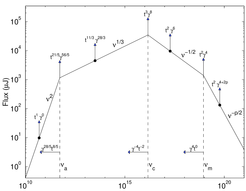
Figure 1: The synchrotron spectrum of power law injected electrons, with cooling and self absorption. The spectrum is made out of four power laws indicated in the figure. The flux at a given (fixed) frequency at each of these segments changes with time as indicated above the up-arrows which begin with a circle. The circle-less arrows, plotted at the break points indicate the scaling of the flux at the break point.

Using the shock jump condition and assuming the electrons and magnetic field acquire a fraction of $\epsilon_{e}$ and $\epsilon_{B}$ of equipartition, we can describe all hydrodynamic and magnetic conditions behind the shock as a function of the observed time $t=t_{s}$sec, the Lorentz factor $\gamma$ and the surrounding density $n_{1}$ cm^-3. The magnetic field $B$ and the typical electron Lorentz factor $\gamma_{e}$ are given by:

$$B=4\gamma\sqrt{2\pi\epsilon_{B}nm_{p}c^{2}},$$ (1)

$$\gamma_{e}=610\epsilon_{e}\gamma.$$ (2)

The typical synchrotron frequency of such an electron is

$$\nu_{m}=1.1\times 10^{19}{\rm Hz}\left(\frac{\epsilon_{e}}{0.1}\right)^{2}\left(\frac{\epsilon_{B}}{0.1}\right)^{1/2}(\frac{\gamma}{300})^{4}n_{1}^{1/2}.$$ (3)

Within the dynamical time of the system, the electrons are cooling down to a Lorentz factor $\gamma_{c}$ where the total energy emitted at a time $t$ is comparable to the electron’s energy: $\sigma_{T}c\gamma^{2}\gamma_{c}^{2}B^{2}t/6\pi=\gamma_{c}m_{e}c^{2}\gamma$. The cooling frequency is the synchrotron frequency $\nu_{c}$ of such an electron:

$$\nu_{c}=1.1\times 10^{17}{\rm Hz}\left(\frac{\epsilon_{B}}{0.1}\right)^{-3/2}\left(\frac{\gamma}{300}\right)^{-4}n_{1}^{-3/2}t_{s}^{-2},$$ (4)

where throughout this paper we use $R\sim 2\gamma^{2}t$, leaving aside corrections of order unity. One can see that for typical parameters, the cooling frequency is lower than the typical synchrotron frequency, except for a very short initial time (0.1 second for $\epsilon_{e}=\epsilon_{B}=0.1$ $\gamma_{0}=300$).

The flux at $\nu_{c}$ is given by the number of radiating electrons, $4\pi nR^{3}/3$ times the power of a single electron:

$$F_{\nu,\max}=220{\rm\mu J}D_{28}^{-2}\left(\frac{\epsilon_{B}}{0.1}\right)^{1/2}\left(\frac{\gamma}{300}\right)^{8}n_{1}^{3/2}t_{s}^{3}.$$ (5)

Finally the self absorption frequency is given by the condition that the optical depth is of order unity i.e.

$$\nu_{sa}=220{\rm GHz}\left(\frac{\epsilon_{B}}{0.1}\right)^{6/5}\left(\frac{\gamma}{300}\right)^{28/5}n_{1}^{9/5}t_{s}^{8/5}.$$ (6)

These scaling are all indicated in figure 1. Note that some of these numbers involve high powers of $\gamma$ and $t$. Therefore, the numerical coefficient given, can be considerably different from the actual value with only a slight change of these parameters. Note that when there are high powers of $t$, the numerical factor in the approximation $t=R/2\gamma^{2}c$ will also affect the numerical result.

The above equation shows that the frequency range for the forward shock, though depends strongly on the systems parameters, is most likely to be around the hard x-ray to $\gamma$-ray regime. This is more or less like the observed GRB. The fraction of the electrons energy that is emitted in optical bands is very small. We shall show later that the reverse shock emission is at a considerably lower frequency, typically around the optical band. However we ignore the reverse shock emission at this stage, and turn to calculate the light curves produced by the forward shock.

3 Light Curves

While the spectrum is always described by the four broken power laws of figure 1, the light curves depend on how the hydrodynamic conditions vary with time. The temporal scaling within each of the spectral segments appearing in figure 1 are given by the up, circle based arrows, when substituting the scaling of $\gamma$ as a function of $t$. These scalings depend on the exact form of the hydrodynamic evolution. Two shocks are formed as the shell propagates into the surrounding material. A forward shock accelerating and heating the surrounding material and a reverse shock decelerating the shell (Rees & Mészáros 1992, Katz 1994, Sari & Piran 1995).

Consider a relativistic shell with an initial width in the observer frame, $\Delta$, and an initial Lorentz factor, $\gamma_{0}$. Sari and Piran (1995) have shown that there are four critical hydrodynamic radii: $R_{s}\sim\Delta\gamma_{0}^{2}$ where the shell begin to spread; $R_{\Delta}\sim(\Delta E/nm_{p}c^{2})^{1/4}$ where the reverse shock crossed the entire shell; $R_{\gamma}\sim(E/nm_{p}c^{2})^{1/3}\gamma_{0}^{-2/3}$ where a surrounding shocked mass smaller by a factor of $\gamma_{0}$ from the shell’s rest mass ($E/\gamma_{0}c^{2}$) was collected; $R_{N}\sim(E/nm_{p}c^{2}\Delta)^{1/2}\gamma_{0}^{-2}$ where the reverse shock becomes relativistic.

We divide the different configurations according to the relative “thickness” of the relativistic shell. The question whether a shell should be considered as thin or thick depends not only on its thickness, $\Delta$, but also on its Lorentz factor $\gamma_{0}$. We will consider a shell thin if $\Delta<(E/nm_{p}c^{2})^{1/3}\gamma_{0}^{-8/3}$. Shells satisfying $\Delta>(E/nm_{p}c^{2})^{1/3}\gamma_{0}^{-8/3}$ are considered thick.

For thin shells the corresponding transition radii are ordered as $R_{s}<R_{\Delta}<R_{\gamma}<R_{N}$. As the shell expands it begins to spread at $R_{s}$. For $R>R_{s}$ the width increases and this causes $R_{\Delta}$ to increase and $R_{N}$ to decrease in such a way that $R_{\Delta}=R_{\gamma}=R_{N}$. So if spreading occurs, by the time when the reverse shock crosses the shell it is mildly relativistic. The corresponding observed time scale of the early afterglow is therefore $t_{\gamma}=R_{\gamma}/2\gamma_{0}^{2}$. This is longer than the burst’s duration, $\Delta/c$, so a separation between the burst and the afterglow is expected (Sari 1997).

For thick shells, the order is the opposite $R_{N}<R_{\gamma}<R_{\Delta}<R_{s}.$ The reverse shock becomes relativistic early on, reducing the Lorentz factor of the shell as $\gamma\sim t^{-1/4}$ (Sari 1997). The radius $R_{\gamma}$ becomes unimportant and most of the energy is extracted only at $R_{\Delta}$, with an observed duration of order $\Delta/c$. The signals from the internal shocks (the GRB) and from the early external shocks (the afterglow) from a thick shell overlap. For thick shells, it might be difficult, therefore, to detect the smooth external shock component.

The final self-similar deceleration phase does not depend on the thickness of the shell. After most of the energy of the shell was given to the surrounding (at $R_{\gamma}$ for thin shells and at $R_{\Delta}$ for thick shells) the deceleration goes on as $\gamma\sim t^{-3/8}$, in a self-similar manner.

To summarize, the hydrodynamic evolution can have two or three stages. In the first stage, the ambient mass is too small to affect the system (the reverse shock is weak) and the Lorentz factor is constant. In the last stage the deceleration is self similar with $\gamma\sim t^{-3/8}$, this stage lasts for months. An intermediate stage of $\gamma\sim t^{-1/4}$ may occur for thick shells only. Most of the energy is transfered to the surrounding material at $t_{\gamma}$ for thin shells or $\Delta/c$ for thick shells.

If internal shocks give rise to the GRB then the observed duration of the burst equals the initial width of the shell divided by $c$. Short bursts correspond to thin shells and long bursts to thick ones. The thickness of the shell in the internal shock scenario is directly observed. Bursts of $20$ sec or longer are likely to belong to the thick shell category. While bursts of duration smaller than $0.1$sec are likely to belong to the thin shell category unless $\gamma_{0}$ is very large ($1500$ or larger). If internal shocks are to produce the bursts, they must occur before the reverse shock has crossed the shell. Since the typical collision radius for internal shocks is $2\delta\gamma_{0}^{2}$, where $\delta$ is the separation between the shells, one needs $2\delta\gamma_{0}^{2}<R_{\Delta}$. This is satisfied automatically for thin shells, for which $2\delta\gamma_{0}^{2}<2\Delta\gamma_{0}^{2}=R_{s}<R_{\Delta}$. However, an additional constraint: $2\delta\gamma_{0}^{2}<(\Delta E/nm_{p}c^{2})^{1/4}$ arises for thick shells, and set an upper limit to the initial Lorentz factor $\gamma_{0}$.

Equations 3-6 show that the self absorbed flux always rises as $t^{1}$. This behavior is independent of the hydrodynamic evolution and it is a general characteristic of fast cooling emission from the forward shock. Therefore, in principle, it can be used as a test of whether the electrons are cooling rapidly or not. However, the self absorbed emission, which is relevant at radio frequencies, is very week in the early afterglow. Detection of radio emission within a few seconds of the burst is unlikely in the near future. Therefore, we will not discuss further the self absorbed frequencies in this paper.

There are many possible light curves. This follows from the appearance of numerous transition between different hydrodynamic evolutions and between the four different spectral segments. Similar to Sari, Narayan and Piran (1998), we define the (frequency dependent) times $t_{c}$ and $t_{m}$ as the time where the cooling and typical frequencies, respectively, cross the observed frequency. Different time ordering of these transitions would lead to different light curves. For thick shells, there are two spectral related times $t_{c}<t_{m}$, as well as two hydrodynamic transitions occurring at $R_{N}<R_{\Delta}$ which corresponds to times $t_{N}<t_{\Delta}$. There are therefore six possible orderings and six corresponding light curves. However, as we have mentioned earlier the initial afterglow signal from a thick shell overlaps the GRB. It will be hard to detect the initial smooth signal of the afterglow and to separate it from the complex internal shocks signal. In addition, as we show later, thin shells can provide more information on the initial Lorentz factor. We will therefore, consider in the rest of the paper only the light curves produce by thin shells.

Thin shells are easier to analyze. Here we have two spectral related times $t_{c}<t_{m}$, but only one additional hydrodynamic time $t_{\gamma}$. At $t_{\gamma}$ the flow changes from a constant Lorentz factor into the self-similar decelerating phase. The thin shell deceleration time, $t_{\gamma}$, is given by

$$t_{\gamma}=R_{\gamma}/2\gamma_{0}^{2}c=\left(\frac{3E}{32\pi\gamma_{0}^{8}nm_{p}c^{5}}\right)^{1/3}$$ (7)

There are only 3 possible light curves. Moreover, it will be easier to distinguish between the GRB and the early afterglow emission from thin shells, as there is a delay between the two.

The light curve is determined according to the time ordering of the different time scales which varies from one observed frequency to the other. We consider, first, high frequencies that are above the initial typical synchrotron frequency (the typical synchrotron frequency with the initial Lorentz factor $\gamma_{0}$):

$$\nu>1.1\times 10^{19}\left(\frac{\epsilon_{e}}{0.1}\right)^{2}\left(\frac{\epsilon_{B}}{0.1}\right)^{1/2}(\frac{\gamma_{0}}{300})^{4}n_{1}^{1/2}.$$ (8)

The typical synchrotron frequency, $\nu_{m}$, depends only of $\gamma$. Since $\gamma$ always decreases with time, then $\nu_{m}$ will decrease with time as well. Therefore, if the observed frequency is initially above the initial typical synchrotron frequency it will remain so during the whole evolution. Consequently, the time $t_{m}$ is not defined for these high frequencies. The light curve in this high frequency regime will be given by $t^{2}\gamma^{4+2p}$ throughout the hydrodynamic evolution (see figure 2a). The light curve rises initially, when $\gamma$ is a constant and then it decreases sharply when $\gamma$ begins to decline.

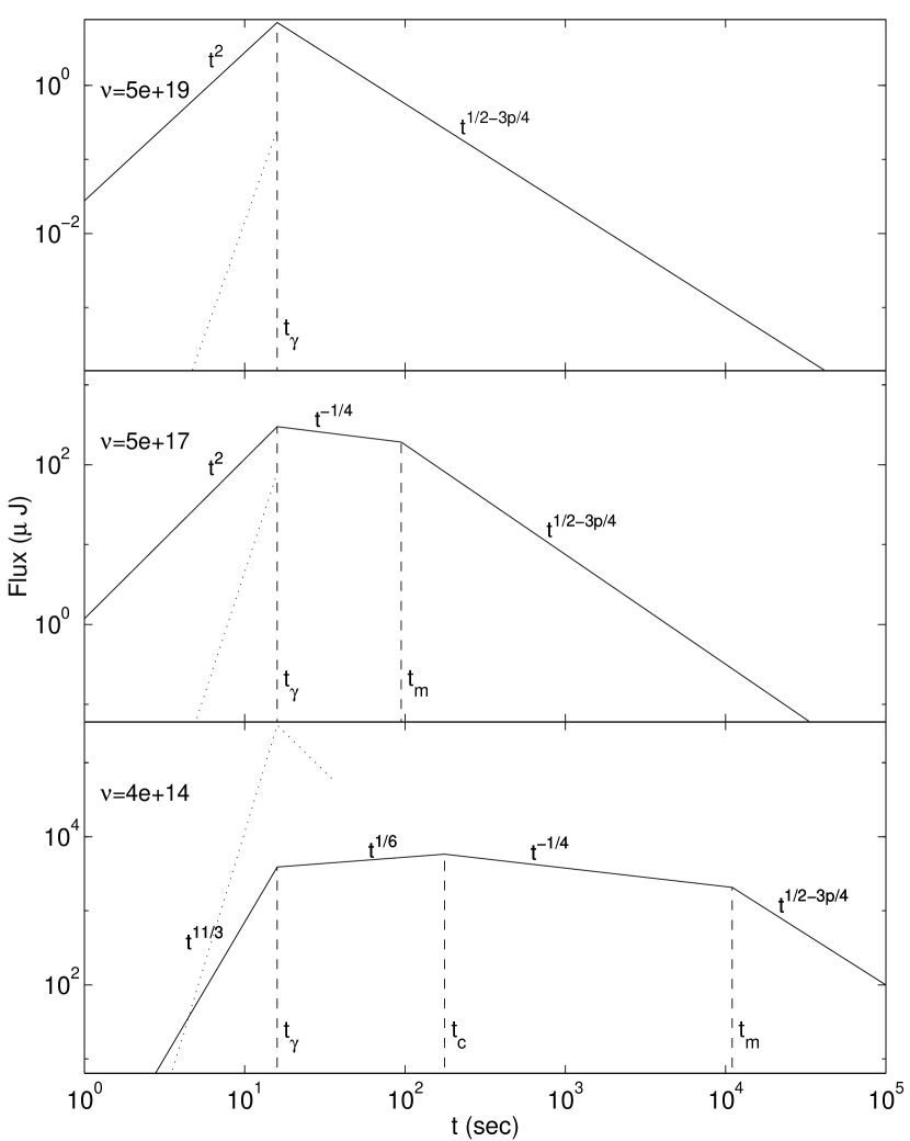
Figure 2: The three possible light curves: high (a), intermediate (b) and low frequencies. For high frequencies, the time $t_{m}$ and $t_{c}$ are undefined since $\nu_{m}$ is below the observed frequency throughout the evolution, and $\nu_{c}$ is crossing the observed frequency on a very short time scale (less than a second), before fast cooling is achieved. In frame (b) the time $t_{c}<1$s therefore not seen in the plot. The dashed line is the emission from the reverse shock. This emission terminates once the reverse shock crosses the shell and the cooling frequency drops below the observed frequency.

The light curve for very low frequencies, which are typically in the optical and possibly the UV, are shown in figure 2c. Low frequencies are defined by the condition: $t_{\gamma}<t_{c}<t_{m}$ or:

$$\nu<2.7\times 10^{15}\left(\frac{\epsilon_{B}}{0.1}\right)^{-3/2}(\frac{\gamma_{0}}{300})^{-4/3}n_{1}^{-5/6}.$$ (9)

At these low frequencies the transition to the decelerating phase occurs before the cooling frequency crosses the observed band and before the synchrotron typical frequency cross the observed band. Although it might be hard to discriminate between the temporal behavior of the almost constant ($t^{1/6}$ ) and $t^{-1/4}$ parts of the low frequency light curves, the spectral shape is very different in these two segments. The spectrum behaves like $\nu^{1/3}$ during the $t^{1/6}$ phase ($t_{\gamma}<t<t_{c}$) while it goes like $\nu^{-1/2}$ during the $t^{-1/4}$ phase ($t_{c}<t<t_{m}$). This spectral change at the time $t_{c}$ should be sufficient to distinguish between the two segments.

For intermediated frequencies, the deceleration begins while the observed band is above the cooling frequency but below the typical synchrotron frequency, i.e. $t_{c}<t_{\gamma}<t_{m}$. The light curve is shown in figure 2b. The relevant range of frequencies are probably in the UV and or soft X-rays, and it is intermediate between those given by the expression 8 and 9.

4 Determination of the initial Lorentz factor

For a short GRB, the time of the afterglow’s peak is given by equation 7. One can invert that to obtain the initial Lorentz factor from an observed time delay:

$$\gamma_{0}=\left(\frac{3E}{32\pi nm_{p}c^{5}T_{0}^{3}}\right)^{1/8}=240E_{52}^{1/8}n_{1}^{1/8}\left(\frac{T}{10{\rm s}}\right)^{-3/8}.$$ (10)

This determination of $\gamma_{0}$ depends only the hydrodynamic transition. Therefore, it is independent of the highly uncertain equipartition parameters $\epsilon_{B}$ and $\epsilon_{e}$ which appear when estimating the spectrum. It is also rather insensitive to $E_{52}$ and $n_{1}$. Moreover, these last two parameters can be determined from late stage observations of the afterglow to within an order of magnitude (Waxman 1997, Wijers and Galama 1998, Granot, Piran and Sari 1998). This equation for $\gamma_{0}$ was used earlier, when it was suggested that GRBs results from an external shock, to estimate the duration of the burst (Rees & Mészáros 1992). However here we assume that the external shocks produce the afterglow while internal shocks produce the burst.

This method, for estimating the initial Lorentz factor depends on the identification of the delayed emission as resulting from the the afterglow rather than just another peak which is part of the burst. It is, therefore, necessary to compare the detailed structure of the delayed emission with the one described in the previous section. A clear characteristic of the early afterglow emissions, in all frequencies, is an initial very steep rise of the emission ($t^{2}$ or even $t^{11/3}$). This happens as the shell collects more and more material and the interaction between the shell and the ISM becomes more and more effective. For the thin shell light curves, discussed in this paper, this initial rise ends at the time $t_{\gamma}$ when the deceleration phase begins. After this rapid rise the light curve becomes almost flat in low and intermediate frequencies, and it decreases rapidly at high frequencies.

It is not clear if such an initial afterglow rise has been observed so far. A good candidate might be GRB970228 (Frontera et. al. 1997, Vietri 1997). This burst consisted of a second peak, mostly in the X-ray range. The statistics for this event may not be good enough to enable a detailed comparison of the light curves around its peak with the theory. However a circumstantial evidence in favor of this explanation exists as the late time X-ray afterglow, extrapolated back in time to the epoch of this second peak, gives the correct flux. Note that a similar situation also exists in GRB970508 and GRB980329, but there the flux does not seem to rise before the second “peak”, so that the rise of the afterglow was not observed. These bursts are probably examples of thick shells.

The identification of the second peak of GRB970228, which occurred $\sim 35$s after the burst, as the afterglow rise yields $\gamma_{0}=150$. The estimated uncertainty is about 50%. This arises from to the unknown values of the energy and the external density, and from the approximations used in the derivation of equations 7 and 10 .

5 Optical Emission and The Reverse Shock

The fluence of a moderately strong burst is $\sim 10^{-5}$ ergs/cm². About one out of 5 of the BATSE bursts are stronger than that, so such a burst occurs once a weak. Were this huge fluence peaking at the optical band rather than in $\gamma$-Rays, with duration of $10$sec, it would correspond to a very bright optical source of flux

$$\frac{1}{4}\times\frac{10^{-5}{\rm ergs/cm}^{2}}{10{\rm s}\times 5\times 10^{14}{\rm Hz}}=50{\rm Jy}\cong 5{\rm th\;magnitude}.$$

The additional factor of 4 in the denominator was chosen to account for the large amount of emission above the peak frequency, which on an average GRB goes as $F_{\nu}\sim\nu^{-1.25}.$ The reason for taking a duration of $10$sec is double: first it is the typical duration of a GRB. Second it is the integration time of fast optical experiments (LOTIS, TAROT), so that even if the emission takes place on a shorter time scale, the effective time will be the observation’s integration time of $10$sec. However, if the emission is spread on a longer time scale, $t_{A}$, then the apparent magnitude will increase accordingly by $2.5\log_{10}(t_{A}/10sec)$.

This is by far stronger than current observational upper limits. In fact, even a small fraction of this will be easily observed. It is therefore worthwhile to explore the expected optical emission at the early GRB evolution.

There are three possible emission regimes which have a comparable amount of energy and could, in principle, emit a powerful optical burst: the GRB itself (whether it is internal or external shocks), the early afterglow produced by the forward shock, and the early emission of the reverse shock. Although, at their peak, each of these sights contains an energy comparable to the total system energy, the optical signal it produces might be dimmer than 5th magnitude for several reasons. The first, as we already mentioned is if the emission is spread in time over a duration longer than $10$s. This is simple to account for and it will increase the magnitude by $2.5\log_{10}(t_{A}/10sec)$. Second, the cooling time might be longer than the system dynamical time and the radiation is not very effective. Third, the typical emission frequency might peak in a different energy band rather than in the optical. The residual optical emission might be significantly smaller. We discuss in the following these two latter effects, and leave farther effects such as inverse Compton scattering and self absorption to the next section.

In contrast to the previous sections, we consider here both the fast cooling and slow cooling synchrotron spectra given by Sari, Piran and Narayan (1998). Ignoring self absorption, there are four (actually five) different cases, which depend on the order of $\nu_{m}$, $\nu_{c}$ and $\nu_{op}$ where the third frequency is a fiducial frequency in the optical band. The fraction of the system’s energy that is emitted in the optical band in those four cases is shown in Table 1.

	$\nu_{c}>\nu_{op}$	$\nu_{c}<\nu_{op}$
$\nu_{m}>\nu_{op}$	$\left(\frac{\min(\nu_{c},\nu_{m})}{\max(\nu_{c},\nu_{m})}\right)^{1/2}\left(\frac{\nu_{op}}{\min(\nu_{c},\nu_{m})}\right)^{4/3^{\phantom{1}}}_{\phantom{1_{1}}}$	$\left(\frac{\nu_{op}}{\nu_{m}}\right)^{1/2}$
$\nu_{m}<\nu_{op}$	$\left(\frac{\nu_{op}}{\nu_{m}}\right)^{-(p-2)/2}\left(\frac{\nu_{op}}{\nu_{c}}\right)^{1/2}$	$\left(\frac{\nu_{op}}{\nu_{m}}\right)^{-(p-2)/2^{\phantom{1}}}_{\phantom{1_{1}}}$

Table 1: The faction of the energy that get emitted in the optical frequency $\nu_{op}$, as function of the cooling frequency $\nu_{c}$ and the typical frequency $\nu_{m}$.

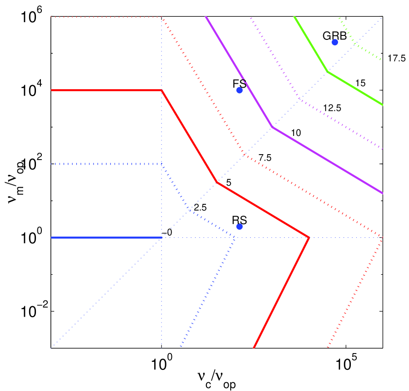
Figure 3: The increase in observed magnitude due to the fact that the electrons are not cooling efficiently and/or the emission does not peak in the optical bands. The three dots represents possible locations of the GRB (GRB), the forward shock (FS) and the reverse shock (RS) in the ($\nu_{c},\nu_{m}$) plane. These locations depend strongly on unknown parameters such as $\gamma_{0}$.

The corresponding increase in the magnitude is shown in Fig. 3, where we have used the “canonical” value of $p\sim 2.5$. With this value of $p$ there is a lot of energy in the high energy tail of the electrons distribution. Consequently the optical emission is rather strong if $\nu_{c}<\nu_{op}$ and $\nu_{m}<\nu_{op}$. Significant suppression occurs only if $\nu_{c}\gg\nu_{op}$ and/or $\nu_{m}\gg\nu_{op}$ with the strongest suppression taking place if both $\nu_{m}\sim\nu_{c}\gg\nu_{op}$.

5.1 The Prompt Optical Burst from the GRB and the Forward Shock

Before turning to the reverse shock, which is our main concern here we examine briefly the prompt optical emission from the GRB and from the forward shock. In both cases the typical synchrotron emission is sufficiently above the optical band and hence we don’t expect significant optical emission from there.

For the GRB we use the observed values of $\nu_{c}$ and $\nu_{m}$. The typical emission frequency during a GRB are mostly between 100keV and 400keV. We will adopt $\nu_{m}=5\times 10^{19}$Hz as a typical value. If the cooling break was below the BATSE band, then the spectral slope within the BATSE band, independent of the electron distribution, would have been $\leq-1/2$. The observed low energy tail is usually in the range of -1/2 to 1/3 (Cohen et. al, 1997). This indicates that the cooling frequency is close to the lower energy of the BATSE band. If the cooling break is indeed in the BATSE range, say at $\sim 30$keV, we can substitute $\nu_{c}=7\times 10^{18}$Hz together with $\nu_{m}=5\times 10^{19}$Hz in table 1, to get that the residual optical emission is of $21$st magnitude. The point that corresponds to these parameters is marked in Fig. 1 as GRB. For bursts which show a low energy tail of spectral index $-1/2$, the cooling frequency is only known to be below the BATSE band. If, on the unlikely extreme, the cooling frequency is much lower, say below the optical band then the optical emission is of $11$th magnitude.

The initial emission of the forward shock, is also characterized by very high typical synchrotron frequency and high cooling frequency (see equations 3 and 4). With reasonable parameters (e.g. $\gamma_{A}\sim 300$, $\epsilon_{e}\sim 0.5$, $\epsilon_{B}\sim 0.1$), this emission is in the MeV range. Consequently the optical emission is fairly weak. Since the same forward shock is also producing the late afterglow, one can scale late time observations to the early epoch to obtain a direct estimate of the early value of $\nu_{c}$ and $\nu_{m}$. Observations carried on GRB 970508 after 12 days show that $\nu_{m,12d}\sim 10^{11}$ Hz and $\nu_{c,12d}\sim 10^{14}$ Hz (Galama et. al. 1998). With adiabatic evolution $\nu_{m}\sim t^{-3/2}$ and $\nu_{c}\sim t^{-1/2}$ so that within $10$s we expect to have $\nu_{m}=3\times 10^{18}$ Hz and $\nu_{c}=5\times 10^{16}$ Hz. With these values we expect the optical emission from the initial forward shock to be of about $15$th magnitude. The point corresponding for these value is marked on Fig 1 as FS. There is some uncertainty in this extrapolation as the initial evolution might be radiative rather than adiabatic. This is considerable only if the value of $\epsilon_{e}\sim 1$ (Sari 1997, Cohen, Piran and Sari 1998). If the evolution is initially radiative, the extrapolation according to the adiabatic scalings is over predicting $\nu_{c}$ while under predicting $\nu_{m}$ (Sari, Piran and Narayan 1998).

5.2 The Reverse Shock Optical Emission

The best candidate to produce a strong optical flash is the reverse shock (Sari & Piran 1999). This shock, which heats up the shell’s matter, operates only once. It crosses the shell and accelerates its electrons. Then these electron cool radiatively and adiabatically and settle down into a part of the Blandford-McKee solution that determines the late profile of the shell and the ISM. Thus, unlike the forward shock emission that continues later at lower energies, this reverse shock emits a single burst with a duration comparable to $t_{A}$ (the duration of the GRBs or a few tens of seconds if the burst is short). After the peak of the reverse shock, i.e. after the reverse shock has crossed the shell no new electrons are injected. Consequently there will be no longer emission above $\nu_{c}$, and $\nu_{c}$ drops fast with time due to adiabatic cooling of the shocked shell material. Therefore, in contrast to the forward shock were we have calculated the whole light curve, we will focus here on the emission at the peak time $t_{A}$.

This peak time is given by

$$t_{A}={\rm\max}[t_{\gamma},\Delta/c]$$ (11)

and the Lorentz factor at this time is

$$\gamma_{A}={\rm\min}[\gamma_{0},(17E/128\pi\Delta^{3}nm_{p}c^{2})^{1/8}]$$ (12)

The afterglow typical time is similar to the duration of the burst (if the burst is long or the initial Lorentz factor is large) or longer than that if the burst was short and the initial Lorentz factor was low. In the latter case the shells Lorentz factor at the time $t_{A}$ equals its initially value $\gamma=\gamma_{0}$, while in the former case some deceleration has already occurred and $\gamma<\gamma_{0}$. After this time, $t_{A}$, a self similar evolution begins, and the initial width of the shell is no longer important. Therefore, the Lorentz factor at the time $t_{A}$, could be estimated in both cases as

$$\gamma_{A}=\left(\frac{17E}{128\pi nm_{p}c^{5}t_{A}}\right)^{3/8}.$$

Before discussing the details of this emission we outline a simple energetic consideration to show that the initial energy dissipated in the reverse shock is comparable to the initial energy dissipated in the forward shock (Sari and Piran 1995) and to the GRB energy. The forwards shock and the reverse shock are separated by a contact discontinuity, across which there is a pressure equality. This means that the energy density in both shocked regions is the same. As the forward shocks compresses the fluid ahead of it by a factor of $\gamma^{2}$ its width is of order $R/\gamma^{2}$. Though the initial width of the shell can be smaller than that, it will naturally spread to this size due to mildly relativistic expansion in its own frame. Since the energy density is the same and the volume is comparable, the total energy in both shocks is comparable. A more detailed calculation (Sari and Piran 1995) shows that at the time the reverse shock crosses the shell about half of the energy is in the shocked shell material.

The two frequencies that determine the spectrum, $\nu_{c}$ and $\nu_{m}$ for the reverse shock are most easily calculated by comparing them to those of the forward shock. The equality of energy density across the contact discontinuity suggests that the magnetic fields in both shocked regions are the same (provided, of course, that we assume the same magnetic equipartition parameter in both regions). Both shocked material move with the same Lorentz factor. Therefor, the cooling frequency, $\nu_{c}$, at the reverse shock is equal to that of the forward shock. However, instead of using the general description of this frequency as function of both $\gamma$ and $t$, we can substitute the expression for $\gamma_{A}$ to get:

$$\nu_{c}=8.8\times 10^{15}{\rm Hz}\left(\frac{\epsilon_{B}}{0.1}\right)^{-3/2}E_{52}^{-1/2}n_{1}^{-1}t_{A}^{-1/2}$$ (13)

The typical synchrotron frequency is proportional to the electrons random Lorentz factor squared (temperature square) and to the magnetic field and to the Lorentz boost. This leads to the $\gamma^{4}$ dependence in equation 3. The Lorentz boost and the magnetic field are the same for the reverse and forward shocks while the random Lorentz factor is $\gamma_{0}/\gamma_{A}$ compared to $\gamma_{A}$ of the forward shock. The “effective” temperature at the reverse shock is much lower than that of the forward shock (by a factor of $\gamma_{A}^{2}/\gamma_{0}\gg 1$). The reverse shock frequency at the time $t_{A}$ is, therefore, given by:

$$\nu_{m}=1.2\times 10^{14}\left(\frac{\epsilon_{e}}{0.1}\right)^{2}\left(\frac{\epsilon_{B}}{0.1}\right)^{1/2}(\frac{\gamma_{0}}{300})^{2}n_{1}^{1/2}.$$ (14)

So while the forward shock radiates initially at the energies of $\sim$MeV the reverse shock radiates at few eV, with significant radiation emission within the optical band.

The case, which is most favorable for a strong optical emission is if the typical frequency of the reverse shock falls just in the optical regime and if the cooling frequency is on or below the optical frequency. This can be achieved with reasonable parameters, say with $n_{1}=E_{52}=1$, $\epsilon_{B}=0.2$, $\epsilon_{e}=0.5$ and $\gamma_{0}=100$. The other extreme case, which has a considerable lower optical fluence is if the typical radiation frequency as well as the cooling frequency are above the optical regime. As is apparent from these last two equations this requires a high initial Lorentz factor, short GRB, high electron equipartition parameter and a low magnetic equipartition parameter.

The resulting optical emission, as function of the most unknown variable $\gamma_{0}$, and for the “best guess” value of the other parameters, as obtained by late afterglow observations, is given in figure 3. As the Lorentz factor increases the optical emission initially rises. This is mainly due to the fact that the emission is spread on a shorter time scale ($t_{A}$ is decreasing). However, with quite a moderate initial Lorentz factor ($\gamma_{0}\sim 300$) the emission duration does no longer depend on the initial Lorentz factor but is given by the observation’s integration time (which we assumed to be $10$sec) or by the duration of the burst (for bursts longer than $10$sec). As the Lorentz factor continues to increase, the emission drops due to the increase in $\nu_{m}$. With high enough values of $\gamma_{0}$ the flux decreases considerably.

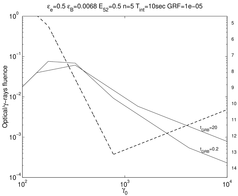
Figure 4: The optical flash from the reverse shock at its peak. The dashed line is the maximal emission allowed by self absorption for burst of duration 0.1s. The self absorption limit for the long burst is too high to fit the y axis.

Two other effect can reduce the flux below these estimates: Self absorption might reduce this flux if the system is optically thick at optical frequencies; Inverse Compton may compete with synchrotron in cooling the electrons and reduce the synchrotron flux. We consider these effects now.

5.3 Synchrotron Self Absorption

Self absorption would reduce the optical flux from the reverse shock if it is optically thick. A simple way to account for this effect, is to estimate the maximal flux emitted as a black body with the reverse shock temperature. This is given by the

$$F_{sa}=\pi(R_{\perp}/D)^{2}S_{\nu}=\pi\left(\frac{R_{\perp}}{D}\right)^{2}\frac{2\nu^{2}}{c^{2}}\frac{\epsilon_{e}}{3}m_{p}c^{2}\gamma_{0},$$ (15)

where the quantity $R_{\perp}\sim\gamma_{A}ct_{A}$ is the observed size of the fireball. More detailed calculations, (Waxman 1997, Panaitescu & Mészáros 1997, Sari 1998, Granot, Piran and Sari 1998a,b) obtain a size bigger by a factor of $\sim 2$. However, these are applicable only deep inside the self-similar deceleration while we are interested in its beginning. To be conservative, we use the lower estimate of the size, which result in a weaker emission. We get that

$$F_{sa}=4.8{\rm Jy}D_{28}^{-2}E_{52}^{1/4}n_{1}^{-1/4}\frac{\epsilon_{e}}{0.1}\frac{\gamma_{0}}{300}\left(\frac{t_{A}}{1s}\right)^{5/4}$$ (16)

Note that so far we have eliminated the dependence on the distance to the burst $D$ by using the observed fluence of the burst. However, self absorption depend on the flux per unit area at the source. The distance, therefore, appears explicitly and can not be eliminated. With a given observed flux, the further the burst is the more important is self absorption. It can be seen from equation 16 that self absorption can hardly play any role for long bursts with say $t_{A}>1$sec. Self absorption can be important only if $t_{A}$ is very short, which is possible only for short bursts and high values of $\gamma_{0}$.

5.4 Inverse Compton Cooling

Synchrotron self-Compton, that is inverse Compton scattering of the synchrotron radiation by the hot electrons provides an alternative way to cool the electrons. The typical energy of a photon that has been scattered is $\nu_{IC}\sim\nu_{m}\gamma_{e}^{2}$. This emission will be in the MeV regime and not in the optical band. However, if $\epsilon_{e}>\epsilon_{B}$ then the efficiency of inverse Compton as a cooling mechanism, relative to synchrotron emission equals: $\sqrt{\epsilon_{e}/\epsilon_{B}}$ (Sari, Narayan and Piran 1996). This will reduce the synchrotron flux of any cooling electron by that factor but will not alter the emitted flux of a non cooling electron. It will therefore influence the optical emission only if $\nu_{c}<\nu_{op}$, and may reduce the flux for this case by a factor of few, resulting in the increase of one or two magnitudes. However, if $\nu_{c}<\nu_{op}$ the reverse shock synchrotron flux is very high to begin with.

5.5 Extinction

In all the discussion above, we have normalized the optical flux according to the observed GRB fluence. However, $\gamma$-rays do not suffer any kind of extinction, while the optical regime may do. Some afterglows show only small amount of extinction, some show strong extinction while other do not show any optical activity and are speculated to be in a highly extincting surrounding. Extinction is probably important if the burst is located in a star formation regime. GRB970508, for example, shows only week extinction after its peak at 2 days. However, before this peak the optical light curve does not fit any of the prediction of the simple models. If this is due to extinction that disappears after two days, it might be crucial in the first few seconds in which we are interested.

6 Discussion

We have calculated the observed synchrotron spectra expected from a relativistic shock that accelerates electrons to a power law distribution for an arbitrary hydrodynamic evolution $\gamma(t)$. Light curves can be obtained from this spectra by substituting initially $\gamma(t)=conts$, then $\gamma(t)=t^{-1/4}$ and finally $\gamma(R)=t^{-3/8}$. Where the intermediate expression relevant only for thick shells. For thin shells, we have explicitly constructed the possible light curves for the forward shock, for several frequency regimes. We find that the flux must rise initially steeply as $t^{2}$ or as $t^{11/3}$. This rapid rise ends at the time $t_{\gamma}$ when the system approaches self similar deceleration. After this time the light curve is either decreasing (high frequencies) or almost flat (low and intermediate frequencies). The break at $t_{\gamma}$ is, therefore, quite sharp and an observational determination of this transition time should be simple.

In the internal-external scenario, thin shells corresponds to short bursts. We expect, in this case, a gap between the burst and its afterglow. This gap allows a clean observation of the early afterglow light curve. In particular we should observe a clear rise, which is not contaminated by the complex, variable internal shocks burst. Thick shells (which correspond to longer bursts) light curves are more complex, due to the overlap of the burst and the afterglow. This overlap would make it difficult or even impossible to isolate the early afterglow signal.

A detection of the early afterglow rise is possible with future missions. Observations of this predicted light curves would confirm the internal shocks scenario. They will also enable us to measure the initial Lorentz factor. Both these ingredients are essential in order to build a reliable source model. As long as the question of internal or external shocks is not settled with a high certainty, it is not clear whether the source deriving the whole phenomena is operating for a millisecond (as required to the fireball needed for the external shock scenario) or for hundred seconds (as required for the internal shocks).

It is important to stress that a detection of a gap in the emission, by it self, is meaningless. The later emission that follows the gap can be just another peak in the complex GRB emission produced by the internal shocks. A comparison between this emission and the theoretical prediction given here is needed in order to unambiguously identify any delayed emission as the beginning of the afterglow rather than as a continuation of the burst. The spectra and light curves described here should be used to discriminate between an additional “delayed” peak, which is just a part of the internal shock burst and an emission coming from an external shock which should be described by the smooth light curves given here.

A broad band detection of the spectrum (say at 1-1000keV), at the time that the afterglow peaks, will enable us to compare between the spectral properties of the GRB and those of the afterglow. In the internal-external picture these spectra are not closely related and the typical synchrotron frequency and cooling frequency emitted in the early afterglow can be either higher or lower than that of the burst. On the other hand, the burst and the afterglow should be similar if the burst itself is also produced by external shocks.

We have calculated the optical emission that is expected in the simplest scenario of creating GRBs. The emission in the optical regime is dominated by the reverse shock. We showed that a strong optical flash is expected over a duration comparable to that of the GRB or delayed a few dozens of seconds after that. We have used the terminology of the internal-external scenario, where the GRB is produced by internal shocks while the afterglow by external shocks. However, even if the GRB is also produced by external shocks, our conclusions are still valid, with $t_{A}$ being the duration of the GRBs itself. The problem in this case, is that the assumption of a uniform surrounding may not be valid for models producing the GRB by external shocks.

The calculations regarding the reverse shock emission assumed that the shell is made out of baryonic material. If instead it is magnetically dominated where the energy in the rest mass of the baryons is negligible, a considerably lower emission is expected from the reverse shock. Our prediction is heavily based on the fact that the reverse and forward shock carry the same amount of thermal energy. If the shell is initially very thin, and somehow does not spread so that its thickness is kept significantly below $R/\gamma^{2}$, the reverse shock will be Newtonian, and will contain a small fraction of the system energy. The emission will be reduced accordingly. In the simplest model, where the shell was accelerated hydrodynamically, the back of the shell moves with a Lorentz factor smaller by a factor of a few from its front (this is what defines the shell) so that spearing to a thickness of $R/\gamma^{2}$ is unavoidable. However, in more complicated forms of acceleration, one might think of shells that have a perfectly uniform Lorentz factor and therefore does not spread.

If the density of the surrounding material is very low, it might take a long time before the shell begins to decelerate, i.e. a very large $t_{A}$. The reverse shock emission will be spread over this large time, resulting in a much lower magnitude. However, it seems to be that this possibility of long $t_{A}$ is already ruled out by current observations, as the beginning of the X-ray decay was observed with BeppoSAX just following some bursts, like GRB 970228, GRB970508 and GRB971214.

Fast optical followup experiments often have a tradeoff between the magnitude they can achieve and how fast can they operate. In this respect, an optical experiment which can detect emission which is simultaneous with the burst is preferred since the reverse shock emission might die soon after that. As there are many bursts of duration of 10 seconds or above, this might be the optimal response time for an optical follow up. Nevertheless, experiments with delays of $30-100$s should still be able to detect the reverse shock emission from a few long enough bursts.

Finally there is the possibility of extinction. At least in some burst, like GRB 970508, extinction does not seem to play a very important roll in the late afterglow. However, the early signal of GRB 970508 (before its peak at two days) is not described well by the theory. If this is an evidence of some extinction, which is important only on early times, it might reduce the optical flash predicted here.

References

- (1) Cohen, E., et. al., 1997, Ap. J., 480, 330.
- (2) Fenimore, E.E., Epstein, R.I., & Ho, C.H., 1993, A&A Supp., 97, 59.
- (3) Granot, J., Piran, T., & Sari, R., 1998, Ap. J., in press, astro-ph/9806192.
- (4) Frontera, F. et. al. 1997, ApJL, 493, L67
- (5) Fenimore, E., Madras, Nayakshin 1996, ApJ 473, 998
- (6) Katz, J.I., 1994, ApJ, 422, 248.
- (7) Kobayashi, S., Piran, T., & Sari, R., 1997, ApJ, 490, 92.
- (8) Mochkovitch, R., Maitia, V., & Marques, R., 1995, in: Towards the Source of Gamma-Ray Bursts, Proceedings of 29th ESLAB Symposium, Eds. Bennett, K., & Winkler, C., 531.
- (9) Panaitescu, A., & Mészáros, P., 1998, Ap. J., 492, 683, astro-ph/9709284.
- (10) Piran, T., 1997, in: Some Unsolved Problems in Astrophysics, Eds. Bahcall, J.N., & Ostriker, J.P., Princeton University Press.
- (11) Piran, T., 1998, Physics Reports, in press.
- (12) Rees, M. J., & Mészáros P., MNRAS 1992, 258 41p.
- (13) Sari, R., 1998, Ap. J. Lett., 494, L49.
- (14) Sari, R., 1997, ApJL, 489, 37.
- (15) Sari, R., & Piran, T., 1995, ApJL, 455, 143.
- (16) Sari, R., & Piran, T., 1997, ApJ 485, 270.
- (17) Sari, R., & Piran, T., 1999, A&A submitted. astro-ph/9901105
- (18) Sari, R., Narayan, R., & Piran T., 1996, ApJ 473 204.
- (19) Sari, R., Piran, T. & Narayan, R., 1998, ApJ 497 L17.
- (20) Vietri, M. 1997, ApJL, 488 L105.
- (21) Waxman, E., ApJL, 1997, 489 L33.
- (22) Wijerse, R.A.M.J. & Galama, T. J. 1998, astro-ph/9805341.
- (23) Woods, E., & Loeb, A., 1995, Ap. J., 383, 292.
- (24)