Can the reionization epoch be detected as a global signature in the cosmic background?

Abstract

The reionization of the Universe is expected to leave a signal in the form of a sharp step in the spectrum of the sky. If reionization occurs at $5\la z_{\rm ion}\la 20$, a feature should appear in the radio sky at $70\la\nu\la 240$ MHz due to redshifted H i 21-cm line emission, accompanied by another feature in the optical/near-IR at $0.7\la\lambda\la 2.6\,\mu$m due to hydrogen recombination radiation. The expected amplitude is well above fundamental detection limits, and the sharpness of the feature may make it distinguishable from variations due to terrestrial, galactic and extragalactic foregrounds.

Because this is essentially a continuum measurement of a signal which occurs over the whole sky, relatively small telescopes may suffice for detection in the radio. In the optical/near-IR, a space telescope is needed with the lowest possible background conditions, since the experiment will be severely background-limited.

1 Introduction

The epoch of reionization marked the end of the “dark ages” during which the ever-fading primordial background radiation cooled below 3000 K and shifted first into the infrared and then into the radio. Darkness persisted until early structures collapsed and cooled, forming the first stars and quasars that lit the universe up again. During this epoch the volume filling factor of ionized hydrogen (H ii) increased rapidly. It is a generic feature of theoretical models and three-dimensional numerical simulations that reionization occurred at $5\la z_{\rm ion}\la 20$ in most cold dark matter (CDM) cosmogonies (Gnedin & Ostriker 1997; Haehnelt & Steinmetz 1998; Cen 1998; Haiman & Loeb 1999).  We know reionization took place before $z\approx 5$, as evidenced by the lack of hydrogen continuum absorption in the spectra of high-redshift quasars (Schneider et al. 1991) and galaxies (Franx et al. 1997). It is unlikely that reionization occurred at $z\ga 50$, for in that case the level of degree scale anisotropy in the CMB would be lower than observed on ten degree scales (e.g. Knox et al. 1998). Tilted and neutrino dominated CDM models give $z_{\rm ion}\simeq$5–8, and open and $\Lambda$-dominated models give $z_{\rm ion}\simeq$7–30 (Cen 1998).

Moreover, since the characteristic distance between the sources that ionized a rapidly recombining intergalactic medium (IGM) was much smaller than the Hubble radius, the transition from H i to H ii was quite abrupt; the overlapping of the H ii regions surrounding the first star clusters and miniquasars was completed on a timescale much shorter than the Hubble time. The reionization epoch occurred almost as a “phase transition” of the Universe. From the observational point of view, this poorly constrained epoch is among the most important unknown quantities in cosmology.

Various techniques for probing the history of the transition from a neutral IGM to one that is almost fully ionized have been proposed in the literature. One way is to look for the 21-cm hyperfine line of neutral hydrogen, redshifted to frequencies in the range 70–240 MHz (Madau et al. 1997; Gnedin & Ostriker 1997; see also Swarup 1984; Swarup & Subrahmanyan 1987; Scott & Rees 1990). Prior to the reionization epoch, the neutral gas that had not yet been engulfed by an H ii region may be seen as 21-cm line emission if a mechanism existed that decoupled the spin temperature from the CMB temperature. Physical mechanisms that would produce a 21-cm signature are Ly$\alpha$ coupling of the spin temperature to the kinetic temperature of the gas, preheating by soft X-rays from collapsing dark matter halos, and preheating by ambient Ly$\alpha$ photons (Madau et al. 1997).

So far the emphasis has been on detecting fluctuations due to individual large H i concentrations. This is very difficult in the presence of a strong fluctuating foreground emission; the H i lines from individual concentrations must be resolved, and this requires large telescopes with high sensitivity and spectral and angular resolution. Alternatively, if reionization occurred abruptly and the fraction of neutral hydrogen underwent a drop of a factor of 10³ in about a tenth of a Hubble time as predicted (e.g. Gnedin & Ostriker 1997; Baltz et al. 1998), it is conceivable that a global signature may be detectable with telescopes of modest size in the extragalactic background spectrum at meter wavelengths. This is in principle a much simpler measurement. Some existing ground-based telescopes may be suitable, or, if terrestrial interference is too severe, a dedicated space project might be considered. A complementary technique is to look for a signal in the optical/near-IR background due to hydrogen recombination radiation from the reionization epoch (Baltz et al. 1998).

The prospects for detecting a global signature of the reionization epoch are considered below. In the following we shall denote the present-day Hubble constant as $H_{0}=100\,h$ km s^-1 Mpc^-1.

2 Reionization signature

Numerical N-body/hydrodynamic simulations of structure formation in a strongly clumped IGM have started to provide a picture for the origin of intervening absorption systems, one of an interconnected network of sheets and filaments, with virialized systems located at their points of intersection. The gas clumping factor rose above unity when the collapsed fraction of baryons became non-negligible, i.e. at $z\la 20$, and grew to a few tens at $z\approx 8$ (Gnedin & Ostriker 1997). This made the volume-averaged gas recombination time,

$$\bar{t}_{\rm rec}=[1.17\bar{n}_{\rm H}\alpha_{B}\,C]^{-1}=0.08\,{\rm Gyr}\left({\Omega_{b}h^{2}\over 0.02}\right)^{-1}$$

$$\left({1+z\over 9}\right)^{-3}C_{10}^{-1},$$ (1)

shorter than that for a uniform IGM and shorter than the the Hubble time at that epoch. In the above expression, $\bar{n}_{\rm H}$ is the mean hydrogen density of the expanding IGM, $\bar{n}_{\rm H}(0)=1.7\times 10^{-7}$ $(\Omega_{b}h^{2}/0.02)$ cm^-3, $\alpha_{B}$ is the recombination coefficient to the excited states of hydrogen, and $C\equiv\langle n_{{H\textsc{ii}}}^{2}\rangle/\bar{n}_{{H\textsc{ii}}}^{2}$ is the ionized hydrogen clumping factor.

When an isolated point source of ionizing radiation turns on, the ionized volume initially grows in size at a rate fixed by the emission of UV photons, and an ionization front separating the H ii and H i regions propagates into the neutral gas. The evolution of an expanding H ii region is governed by the equation

$${dV_{I}\over dt}-3HV_{I}={\dot{N}_{\rm ion}\over\bar{n}_{\rm H}}-{V_{I}\over\bar{t}_{\rm rec}},$$ (2)

(Shapiro & Giroux 1987), where $V_{I}$ is the proper volume of the ionized zone, $\dot{N}_{\rm ion}$ is the number of ionizing photons emitted by the central source per unit time, and $H$ is the Hubble constant. Across the ionization front the degree of ionization changes sharply on a distance of the order of the mean free path of an ionizing photon. When $\bar{t}_{\rm rec}\ll t$, the growth of the H ii region is slowed down by recombinations in the highly inhomogeneous IGM, and its evolution can be decoupled from the expansion of the universe. As in the static case, the ionized bubble will fill its time-varying Strömgren sphere after a few recombination timescales,

$$V_{I}={\dot{N}_{\rm ion}\bar{t}_{\rm rec}\over\bar{n}_{\rm H}}(1-e^{-t/\bar{t}_{\rm rec}}).$$ (3)

While the volume that is actually ionized depends on the luminosity of the central source, the time it takes to produce an ionization-bounded region is only a function of $\bar{t}_{\rm rec}$.

At early times, the characteristic distance between the sources that ionized a rapidly recombining IGM was much smaller than the Hubble radius. The phase transition from H i to H ii was therefore quite abrupt. When the H ii regions surrounding the first star clusters and miniquasars overlapped, the fraction of neutral hydrogen dropped by a few orders of magnitude in about a tenth of the Hubble time at that epoch, the continuum optical depth decreased suddenly and the background ionizing intensity underwent a drastic increase in a very small redshift interval (Gnedin & Ostriker 1997; Baltz et al. 1998). The redshift of this event is expected to be essentially the same in all directions. It is this abrupt change in H i absorption that flags the epoch of reionization and may be observable at radio and optical/near-IR frequencies, as shown below.

3 Detectability of an H i edge

The intergalactic medium prior to the epoch of full reionization should be detectable in 21-cm line radiation. In the absence of a decoupling mechanism, the spin temperature of neutral hydrogen would go to equilibrium with the CMB, and no emission or absorption relative to the CMB would be detected. The collapse and cooling of the first non-linear structures had a twofold effect: (1) it preheated the IGM to temperatures $\sim 150$ K, above that of the CMB; and (2) through scattering by Ly$\alpha$ photons it provided a mechanism to couple the spin temperature to the kinetic temperature of the gas (Madau et al. 1997). A patchwork – due to large-scale structure and non-uniform heating and coupling – of 21-cm line emission would result, a signal which would have disappeared after reionization. A signature (“step”) in the continuum spectrum of the radio sky, at a frequency of $\sim 70-240$ MHz for $z_{\rm ion}$ in the range 5–20, will therefore flag the reionization epoch.

To illustrate the basic principle of the observations we propose, consider a neutral IGM with spin temperature $T_{S}\gg T_{\rm CMB}$. In an Einstein-de Sitter universe ($\Omega_{0}=1$, $\Omega_{\Lambda}=0$), its intergalactic optical depth at $21(1+z)\,$cm along the line of sight,

$$\tau(z)\approx 10^{-3}h^{-1}\left({T_{\rm CMB}\over T_{S}}\right)\left({\Omega_{b}h^{2}\over 0.02}\right)(1+z)^{1/2},$$ (4)

will typically be much less than unity. The experiment envisaged consists in its simplest form of two measurements separated in frequency such that the one at shorter wavelengths detects no line feature because all hydrogen has been reionized. The differential antenna temperature across the “step”, as observed at Earth, will be

$$\Delta T=(1+z)^{-1}(T_{S}-T_{\rm CMB})(1-e^{-\tau})\leavevmode\nobreak\ \leavevmode\nobreak\ \leavevmode\nobreak\ \leavevmode\nobreak\ \leavevmode\nobreak\ \leavevmode\nobreak\ \leavevmode\nobreak\ \leavevmode\nobreak\ \leavevmode\nobreak\ \leavevmode\nobreak\ \leavevmode\nobreak\ \leavevmode\nobreak\$$

$$\approx(0.01\leavevmode\nobreak\ {\rm K})h^{-1}\left({\Omega_{b}h^{2}\over 0.02}\right)\left({{1+z_{ion}}\over 9}\right)^{1/2},$$ (5)

where $z_{ion}$ is the redshift of the transition epoch. Note that in a universe with $\Omega_{0}\ll 1$, $\Delta T$ increases more nearly linearly with $(1+z_{ion})$, and the numerical coefficient in Eq. (5) may be larger by up to a factor $3[(1+z_{ion})/9]^{1/2}$. Depending on the cosmology, $\Delta T$ will increase toward low frequencies at a rate between $\nu^{-1/2}$ and $\nu^{-1}$. Hence, the expected cosmological signal will be an edge of more than $\sim$ 0.02 K (for $h=0.5$) at 70–240 MHz superimposed on the 2.73 K cosmic background radiation. Fig. 1 shows the total cosmological signal, comprised of the cosmic background radiation with the reionization step superimposed.

3.1 Fundamental sensitivity limits

The fundamental limitation on the sensitivity achievable is set by the intensity of the galactic and extragalactic foregrounds. Modern receivers are such that the system temperature should be largely dominated by these extraterrestrial signals. The limiting sensitivity is thus

$$\Delta T_{\rm min}\sim\frac{T_{\rm sys}}{\sqrt{\delta\nu t}},$$ (6)

where $T_{\rm sys}$ is the total system temperature, $\delta\nu$ is the bandwidth, and $t$ is the integration time. For $T_{\rm sys}$ = 150K (the coldest regions of the sky at 150 MHz) with a bandwidth of 5 MHz and integration time 24 hours, $\Delta T_{min}$ $\sim$ 0.0002 K. The reionization step predicted by Eq. (5) would be $\sim$ 100$\sigma$, independent of telescope size. In a real measurement the system temperature would of course be higher than this fundamental limit of 150K, but clearly sensitivity is not an issue, and the challenge concerns signal contamination and calibration, as discussed below.

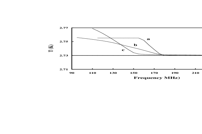
Figure 1: Expected brightness temperature of the cosmic background in the vicinity of the H i reionization edge as a function of observing frequency. Three cases are shown for the H i step, (a): the case from Eq. (5) with $z_{ion}$ = 7, $\Delta z$ = 1 and $h=0.7$, (b) and (c): revised results provided by N. Gnedin (private communication) from the simulations by Gnedin & Ostriker (1997) and Baltz et al. (1998) case A respectively, with $\Omega_{M}=0.35$, $\Omega_{\Lambda}=0.65$, and $h=0.7$.

3.2 Contamination by galactic and extragalactic foregrounds

The difficulty posed by the galactic and extragalactic foregrounds is that they can be complex, both in frequency and position. The question is whether one can in principle extract a 0.02K step from this much stronger varying continuum.

All-sky maps at 150 and 408 MHz are presented in Landecker & Wielebinski (1970) and Haslam et al. (1982). The regions of lowest brightness temperatures occur in large, relatively smooth regions away from the galactic plane and galactic loops. This emission is comprised of four components: galactic synchrotron emission ($\sim$ 70% at 150 MHz), galactic thermal (free-free) emission ($\sim$ 1%), the integrated emission from extragalactic sources ($\sim$ 27%), and the 2.73 K cosmic background itself.

The galactic nonthermal synchrotron emission is dominant at these low frequencies, and has been studied since the pioneering days of radio astronomy. Its spectrum is close to a featureless power law, although there are gradual variations in the spectral index with position on the sky and with frequency. The spectral index is smallest in the coldest regions of the sky, away from the galactic plane and galactic loops. Variations appear to be mainly due to the latter. At 100 MHz the spectral index $\beta$ of this component is about –2.55 in cold sky regions, and it steepens to –2.8 at 1 GHz (Bridle 1967; Sironi 1974; Webster 1974; Cane 1979; Lawson et al. 1987; Reich & Reich 1988; Banday & Wolfendale 1991; Platania et al. 1998). In some regions such as the north galactic pole this steepening of the spectrum appears to be considerably less pronounced (Bridle 1967).

There may also be a dispersion in the spectral index at each position on the sky, due to distinct components along the line of sight. Some indication of this dispersion is given by point-to-point variations of the spectral index over the sky (Landecker & Wielebinski 1970; Milogradov-Turin 1974; Lawson et al. 1987; Reich & Reich 1988; Banday & Wolfendale 1990, 1991). It is not large, and appears to be smallest at the lower frequencies (Lawson et al. 1987; Banday & Wolfendale 1990). A value of $\sigma(\beta)\sim$ 0.1 is probably appropriate at 100–200 MHz. Further information on small-scale uniformity can be provided by simultaneous interferometric data on many short baselines using telescope arrays such as the WSRT and GMRT. The recently completed Westerbork 325 MHz survey of the northern hemisphere (WENSS, de Bruyn et al. 1998) already gives some constraints. At high galactic latitudes, where the minimum brightness temperature of the diffuse galactic emission is about 20 K at 325 MHz, the variations in the brightness temperature of the galactic foreground emission are typically less than about 0.4 K, or about 2%, on scales ranging from 5–30 arcmin. If spatial intensity variations are accompanied by spectral variations (as they would be, if caused by low surface brightness H ii regions or supernova remnants), such measurements can be used to set limits on spectral variations.

The galactic thermal emission at high galactic latitudes is due to very diffuse ionized gas, with total emission measure about 5 pc cm^-6 for $T_{e}$ = 8000K (Reynolds 1990). More recent studies of the properties of this gas have been made by Kogut et al. (1996) and de Oliviera-Costa et al. (1997), who show that it has structure correlated with high-latitude dust clouds. This gas is optically thin at frequencies above a few MHz, so its spectrum in the region 100–200 MHz is well-determined, with a spectral index of –2.1.

Spectral lines present a related potential contamination. Galactic radio recombination lines occur every 1-2 MHz over the frequency range of interest. In addition to spontaneous emission from ionized hydrogen and other elements in the clouds, there is also stimulated emission (or absorption) against the nonthermal background. Peak line intensities can reach 1K or so, although it turns out that the galactic ridge recombination lines happen to make the transition from emission to absorption at 100–200 MHz, and so are at a minimum in this range (Payne et al. 1989). Even a line intensity of 1K becomes diluted to 0.002K in a 5 MHz band. In any case, spectral lines can be identified and removed with observations of higher spectral resolution. Observations such as these may provide the added bonus of discovering or setting limits on presently unknown spectral lines.

The isotropic emission from extragalactic sources has been estimated both directly and from integrated source counts. Bridle (1967) found that this component amounts to about 48K at 150 MHz, with a spectral index of –2.75. Cane (1979) obtained a value corresponding to about 32K at 150 MHz, based on observations at 10 MHz. This is consistent with results from integrating the source count data (Willis et al. 1977; Simon 1977; Lawson et al. 1987). Simon (1977) estimated that the total extragalactic background should turn over between 1 and 2 MHz due to synchrotron self-absorption in the individual source components, but individual sources can have complex frequency structure at much higher frequencies. In the extreme, spectral indices can range from +2 (sources with sharp synchrotron self-absorption turnovers) to –3 (pulsars). Overall, the resulting features in the extragalactic background should be small and slowly varying functions of frequency due to source inhomogeneities and the average over many sources.

This has been simulated using the known spectral properties of 3C sources as studied by Kellermann et al. (1969). They classified the spectra of almost all 3C sources in the following categories: S (straight – single power law), C– (convex – steepening at higher frequencies), C+ (concave – flattening at higher frequencies), and Cpx (complex – containing multiple components). Of the 299 extragalactic sources studied, 42% are S, 52% are C–, 3% are C+, and 3% are Cpx. The actual spectral shapes of 37 3C sources representing all these classes were measured from spectra published in Kellermann (1966, 1974), Kellermann et al. (1969), Kellermann & Pauliny-Toth (1969), and Kellermann & Owen (1988). These were then weighted in accordance with the frequency of occurance of the various classes, and co-added to give a representative composite spectrum of the extragalactic foreground.

The resulting extragalactic spectrum in the range 50-300 MHz is close to a power law of spectral index –2.65 (the index is steeper at higher frequencies). The deviation from this power law is a slowly and continuously varying function of frequency, with an index ranging from –2.59 to –2.66 and no sharp features. The smoothness of this spectrum based on just 37 sources (see Fig. 3) is reassuring, as vastly more sources will contribute to the real extragalactic signal, which will be correspondingly more featureless. The overall spectrum of the real extragalactic signal will differ from that computed here, as only the most luminous sources are represented in this simulation, but the important conclusion is that the spectrum should be smooth and featureless.

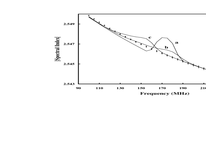
Figure 2: Spectral index vs. observing frequency, as deduced over 10 MHz intervals from simulated spectra which include the galactic nonthermal emission with median spectral index $\beta$ = -2.55 and a Gaussian dispersion around this value with $\sigma$ = 0.1, and the galactic thermal emission with $EM$ = 5 pc cm^-6 and $T_{e}$ = 6000K, in addition to the reionization signal (the constant 2.73K cosmic background has been removed). The emission from extragalactic sources is omitted in this case. The total brightness temperature at 150 MHz is 150K. The points represent the case without a reionization step, and the error bars correspond to $\pm 5\sigma$ for a 24-hour observation. The lines represent the three cases shown in Fig. 1.

Nevertheless it will still be important to identify and characterize the spectral properties of the dominant sources within the main beam. Interferometer observations can be made for this purpose. A single source with a flux density of 35 mJy at 150 MHz would produce an antenna temperature increase of 0.01 K for a 45m telescope with 50% main beam efficiency. All sources should therefore be identified down to at least this level. The GMRT would be the instrument of choice to conduct these high resolution observations. With receivers for 50, 150, 235 and 325 MHz and a resolution of better than 1’ (at 50 MHz), spectra of all significant sources can be determined in the relevant frequency range.

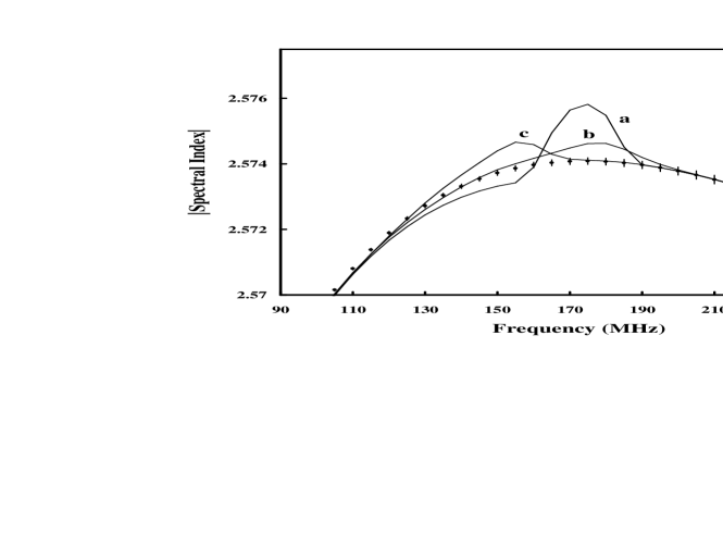
Figure 3: Spectral index vs. observing frequency as in Fig. 2, except that in this case the emission from extragalactic sources is included, represented by the simulation described in the text based on the actual spectra of 37 3C sources. Again, the total brightness temperature at 150 MHz is 150K.

Thus, it may be possible to quantify all the foreground contaminants sufficiently to model them and possibly remove some of them. The fact that the reionization signal should be the same over the whole sky is a great advantage - searches in different positions on the sky with different contamination should give the same result. A range of different measurements can help greatly in disentangling these foreground signals. Accurate broadband spectra over a wide frequency range can help to determine the spectral behavior of the galactic nonthermal component, and measurements in adjacent positions can constrain the dispersion of the spectral index. High frequency measurements can be used to accurately determine the galactic thermal component. Interferometer observations can be used to identify regions devoid of strong extragalactic sources, and to measure the properties of the most prominent sources in the regions chosen.

The analysis can be done in a number of ways, depending on how effectively the different components can be modeled or removed. If the overall spectrum could be well determined at frequencies above that of the reionization step (e.g. $\nu>$ 237 MHz, corresponding to $z<5$), a simple extrapolation to lower frequencies could be made to find the step. It is unlikely, however, that such an extrapolation could be made with sufficient reliability. Alternatively, after those components that are well-determined have been removed (at least the 2.73 K cosmic background and the galactic thermal emission), a best fit (power law or low-order polynomial) could be made and subtracted or divided from the actual spectrum to reveal the step, although the fit may well introduce artifacts that can mask or confuse the signal. A natural approach is to make the fit at the two ends of the spectrum and interpolate, but this requires a well-behaved spectrum and assumes that the signal is located near the middle of the spectrum. Another possibility is to measure the spectral index point-by-point along the spectrum, and look for an abrupt jump due to the step.

Figure 2 shows the spectral index measured every 10 MHz from simulated spectra containing just the galactic thermal and nonthermal emission in addition to the reionization signal. In Fig. 3 the extragalactic sources have been included. These two examples give an idea of the range of spectral curvature that can be expected. The overall curvature is substantial, but the reionization signal can still be seen in all three cases because of its relative sharpness.

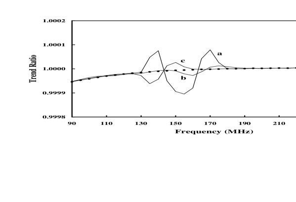
Figure 4: The “trend ratio” as described in the text, computed for the curves used in Fig. 3, plotted against observing frequency.

Another technique that does not involve any fitting procedure (but does require high-precision measurements) is trend analysis – analyzing the spectrum for deviations from a smooth trend. Fig. 4 shows the ”trend ratio”, defined here as the ratio of the observed brightness temperature at a given frequency to that predicted from an extrapolation of the brightness temperatures measured at the three higher frequency points. The disruption caused by the reionization signal to the otherwise smooth spectrum is obvious.

Clearly, both the magnitude and sharpness of the reionization step are critical parameters. As mentioned at the beginning of Sect. 3, the magnitude of the step will be greater in a low density Universe. The sharpness depends on the clumpiness of the Universe at the reionization epoch and the formation rate of the ionizing sources, and may well be greater than indicated by curves (b) and (c). Simulations of the evolution of structure can give some indication of these parameters, but ultimately they have to be determined from observations.

In summary, it appears that the reionization step may be detectable in principle, even in the presence of contamination due to the galactic and extragalactic foregrounds. How easily it can be detected, and which method of analysis is best, will depend on how well the different contaminating components can be measured, modeled and removed. For this purpose, new and accurate studies of these foreground contaminants will be very important. The remaining limitations are then purely technical, and present an interesting challenge. Some of the practicalities are discussed below.

3.3 Observational prospects

3.3.1 Telescope requirements

As (1) the signal is present over the entire sky, (2) the system temperature is dominated by the galactic and extragalactic nonthermal emission, and (3) this is a broadband (rather than line) observation, this experiment can in principle be done using already existing radio telescopes of moderate aperture. The main requirement is to achieve highly accurate relative intensity measurements over a considerable frequency range (70–240 MHz).

Attractive as the use of a small telescope for this measurement may be, however, there are significant difficulties. The gain of the telescope, its beamshape and its (distant) sidelobes are frequency-dependent, due to matching, feed illumination, feed support scattering and edge-refraction effects. The beamsize increases with decreasing frequency, so the regions contributing to the galactic and extragalactic emission are different at different frequencies. This will further complicate the shape of the overall spectrum, although the effect should vary slowly and smoothly with frequency, particularly in the directions of lowest galactic emission. The distant sidelobes may also introduce (varying) signals from regions of stronger galactic emission.

The large beam of a small telescope would average over the effects of many extragalactic sources, and more sources would be included at lower frequencies where the beam is larger. Averaging over many sources could conceivably be an advantage, as long as a small number of sources did not dominate, but with a larger telescope and smaller beam it would be easier to observe in regions devoid of strong extragalactic sources. Finally, if a strong source such as Cas A is to be used as a calibrator (see below), a fairly large antenna is required for the signal from this source to dominate over the surrounding galactic emission.

A larger parabolic antenna would solve some of these problems, but not all. Some sort of phased array with beam-forming circuitry which is still sensitive to emission on the largest scales may have several advantages. It would be possible to use scaled beams at all frequencies and control sidelobes, so that exactly the same area of sky would be sampled at all frequencies. New arrays of this type, such as the THousand Element Array (THEA) in The Netherlands and the Square Kilometer Array (SKA) are presently under consideration (van Ardenne 1998).

If terrestrial complications such as radio-frequency interference were considered insurmountable, one might consider a small satellite project. Then there would be only the galactic and extragalactic foreground contamination to contend with, as well as calibration (although solar radiation may also be a significant problem). The antenna size would obviously be limited, but even a deployable 10m antenna, giving a 10^∘ beam at 180 MHz, may be adequate. At these frequencies the precision of the antenna surface would not be an issue. While space projects are not inexpensive, a space radiotelescope such as this may find novel uses, as it would be exploring a new domain in observational phase space.

3.3.2 Calibration options

To be specific we will discuss three different calibration strategies, and mention specific problems for each of them and how they might be solved. Calibrating the frequency response of the telescope/receiver combination is probably the crucial issue. This has to be done to better than a few parts in 10⁵ over a wide frequency range. Possibilities (which could be combined) include internal loads, or the use of astronomical sources - a very strong ’featureless’ continuum source such as Cas A, or the moon. We discuss each of these in turn.

a) Internal loads

For precise calibration over many frequency channels, internal broad-band noise sources of the highest quality would undoubtedly be the best option. They would have to be extremely stable and very accurately calibrated as a function of frequency. The properties of available internal calibration sources will have to be examined carefully to determine whether this is an option – until now, calibration of this accuracy and stability has not been required at these frequencies, so this is uncharted territory. Calibration with an internal load must also take care of any frequency dependence of the load-coupling into the signal path.

b) Using Cas A

The alternative is to use astronomical calibration sources. This has the advantage that the astronomical signal and the calibration signal both traverse the same path through the telescope and receiver system and therefore share similar gain-frequency effects. Cas A is the strongest source in the sky at 150 MHz, with a flux density of 13,000 Jy. In order for this source to produce an antenna temperature well in excess of the local galactic emission (Cas A sits on the galactic ridge), a telescope of 25m diameter or more would be required. The use of such a source may introduce a further complication: although its overall power-law spectrum is remarkably straight down to a few MHz (Baars et al. 1977), many small components with a range of spectral indices are superimposed, modifying the detailed overall spectrum to an extent yet to be determined (Anderson & Rudnick 1996, and references therein). Strong extragalactic sources such as Cygnus A have more complex, curved spectra (Baars et al. 1977), and so may be less suitable as calibrators.

Probably the best existing telescope to begin with is the GMRT. Cas A would produce an antenna temperature of about 4300 K at 150 MHz with the 45m antennas, totally dominating the sky and receiver noise. The GMRT has receivers over a wide range of frequencies, but not contiguous over the desired range from 70–240 MHz. Total power measurements, accompanied by autocorrelation spectra of the input signals to identify data affected by narrow band interference, are required. Digital spectrometers with at least 20-40 MHz bandwidth and several thousand spectral channels would be needed.

c) Using the moon

An advantage of the moon over Cas A is that it moves, and a true differencing experiment could therefore be done at exactly the same position(s) in the sky, and in the same alt-az position(s), but of course not at the same time. All stable contaminating effects (galaxy, discrete sources, sidelobes etc) will to first and perhaps second order be identical and will cancel, leaving only time-dependent concerns - overall stability and radio-frequency interference. A true differencing experiment such as this may be very attractive in coping with the contribution to the system temperature coming in via distant sidelobes. It will be hard to limit this contribution to less than 50 K at the low frequencies of this experiment. This component may have significant frequency structure which could be difficult to model. This may be a great advantage of using the moon compared to an experiment using Cas A.

The brightness temperature of the moon is about 220 K in this frequency range (Keihm & Langseth 1975); it varies slowly with lunar phase. This is close to the minimum sky temperature at 150 MHz, so if the moon fills the beam it will not increase the antenna signal by much, if at all. The fact that the moon completely blocks the emission behind it (galactic and extragalactic) can be very useful, and could help solve the problem of the frequency-dependent beamsize. The moon is not a very bright calibration source so it takes a large telescope to avoid diluting the signal too much. For the moon to fill the beam, we require a telescope of about 200–400 m diameter at the frequencies that we are considering. Currently only Arecibo would be able to provide a sufficiently narrow beam. A specially designed low-frequency phased-array, such as those mentioned in Sect. 3.3.1, may be required.

An interesting aspect of a moon calibration experiment is that the detection of the signal could in principle be done interferometrically. Because the moon occults the background signal it introduces spatial structure in the global edge signal. Depending on the frequency and the intensity of the galactic background, the 220 K moon could be a colder or warmer spot in the sky. But the intensity of this negative or positive source contains the frequency-dependent global background temperature.

Of course, the motion of the moon also introduces smearing effects, which would probably be advantageous. If the ’edge’ signal is universal, as expected, we need not worry that the moon moves by approximately its diameter every hour. Both the sought-after signal and the sidelobes will be averaged. Since we need to integrate over many (tens of) hours by tracking the moon we are effectively sensitive only to a large-scale signal. The possibility that emission from the moon, which includes a time-variable contribution from scattered solar radiation, may have weak frequency structure will have to be investigated.

Alternatively (especially if smaller telescopes are used) even the sun might conceivably serve for calibration purposes. Although the solar spectrum has considerable frequency structure during bursts, the quiet sun is less likely to have permanent spectral features at 70–240 MHz, since we are looking well into the “quiet” spectrum of the solar chromosphere superimposed on the Rayleigh-Jeans tail of its 6000 K atmosphere. Several issues will have to be further studied before deciding on the optimal calibration strategy.

3.3.3 Terrestrial interference and complications

Radio-frequency interference (RFI) is of course a major issue for observations at the frequencies of interest. The World Radio Conference had allocated only one protected radio astronomy band in this regime, at 150–153 MHz, which itself is already severely affected by interference (Spoelstra 1998). This region of the radio spectrum is subject to local, regional and world-wide interference. Some of these are stationary sources of interference such as TV stations, many other in the 100–200 MHz regime are of a mobile nature such as aeronautical and military transmitters and beacons. Fortunately, many of these sources are strongly time-variable and confined to relatively narrow bands. The 88–108 MHz band is allocated to FM radio and may be completely inaccessible for radio observations of the required accuracy. This means that if the H i ’edge’ signal is at redshift greater than 10 (i.e. at frequencies less than 130 MHz) there may not be a reliable spectral baseline left.

It is interesting to consider the role that could be played by interferometers in this experiment. Such arrays can, with many independent monitors of the total power, provide an excellent discriminator (filter) for local or external RFI. Because RFI generally does not come from the direction of the signal its delay and fringe rate will also be different. This then provides a way of detecting and possibly eliminating RFI, so using telescopes that are part of an interferometric array may yield powerful diagnostic capabilities for weak RFI.

Ionospheric effects are also important at these frequencies. The ionosphere not only refracts the signal by a varying amount (easily 1-2 arcminutes) but there is also refractive focussing and scintillation. These scale with frequency in a quadratic way. However, the ionosphere changes daily, so one can always select the best conditions. The effects would be of greatest concern for the observations of the discrete calibration sources, and should not be important for low-resolution observations of the frequency dependence of large areas of sky.

4 Detectability of a Lyman reionization edge

In this section we discuss the possibility of detecting the reionization edge via the Lyman lines. We first discuss the nature of this optical/IR signal, next its observability in general, and then we conclude by discussing an experiment with existing equipment.

The rate of hydrogen recombinations peaks at $z\simeq z_{\rm ion}$, and this is the source of the background we seek. Because we want to observe a spectral signature in the all-sky background, we are only concerned with how energy is redistributed among different spectral lines. Baltz et al. (1998) showed that intergalactic absorption brightens some lines while it dims others. At $z\geq z_{\rm ion}$, the optical depth in the Lyman series is very high. All Lyman series lines except Ly$\alpha$ are absorbed immediately and redistributed. This makes Ly$\alpha$ and the Balmer series significantly brighter, because they receive the energy of the Lyman series. Once reionization occurs, the Lyman series becomes optically thin and the brightness of Ly$\alpha$ and the Balmer series drops considerably, producing sharp features in the background spectrum.

If reionization occurs abruptly, such a sharp edge may be observable as a global signal over the entire sky due to Ly$\alpha$ emission at z$\simeq$5–20 ($\lambda\simeq$0.7–2.6$\mu$m). This can be seen from the models of Baltz et al. (1998) shown in Fig. 5. As we look redward, crossing Ly$\alpha$ around $\sim$1$\mu$m during the reionization event, the brightness suddenly increases due to the absorption and redistribution of the higher Lyman series lines. Haiman et al. (1997) calculated a similar effect in which Ly$\alpha$ is brightened by radiative excitations, but it appears that recombination gives a significantly stronger signal. Baltz et al. (1998) and Longair (1995) estimate the strength of the edge to be in the range $J_{\nu}({\rm Ly})\simeq 0.3-3\times 10^{-23}$ erg/cm²/s/Hz/sr (these estimates are probably uncertain by $\ga$ 0.5 dex).

Further recombination features are also present in the spectra in Fig. 5. The broad humps (most noticeably that blueward of Ly$\alpha$) are due to blends of lines from the Lyman and Balmer series (Baltz et al. 1998; see also Stancil et al. 1998 for other possible transitions with lower probability). The positions of these humps are of course fixed relative to the sharp features. Their shapes are determined by the evolution of the reionization/recombination history.

Figure 5: Predicted spectra of the Lyman reionization edge from Baltz et al. (1998). Models A–D were generated from CDM simulations including radiative transfer, star-formation, feedback, evolution and chemistry of the gas, and assume $\Omega_{M}=0.35$, $\Omega_{\Lambda}=0.65$, and $h=0.7$. The sequence A–D has decreasing values of $\Omega_{b}$ (0.055-0.03), simulation box-size (3–2 h^-1 Mpc), mass resolution ($10^{7.0}$–$10^{6.0}$ $M_{\odot}$), and number of particles. The amplitude prediction in the models is probably uncertain by $\ga$ 0.5 dex. The most noticeable hydrogen edges, Ly$\alpha$ and H$\alpha$, are indicated (for model D only). The hump blueward of Ly$\alpha$ is caused by higher atomic transitions. The dotted curves indicate the in-principle 3-$\sigma$ limits expected from a day of integration with HST/STIS, HST/WFC3, NGST, and a long integration on a similar spacecraft at 3 AU from the sun. The uncertainty in these limits are about $\sim$0.3 dex.

4.1 Fundamental sensitivity limits

The sky brightness at these wavelengths is dominated by the zodiacal light. The Diffuse Galactic Light (DGL), and the Extragalactic Background Light (EBL) also contribute, but at a lower level. These “foreground” emissions determine the fundamental sensitivity limits for this observation.

The dominant foreground signal is the zodiacal “background”, which at high galactic and ecliptic latitudes is well determined by HST in the WFPC2 B, V, I bands at $\sim$23.9, 23.00, and 22.45 arcsec^-2, respectively (Windhorst et al. 1992, 1994b, 1998), and $\ga$20.9 and $\ga$19.6 mag arcsec^-2 in the Near-Infrared Camera/Multi Object Spectrograph (NICMOS) near-IR J and H bands, respectively (Thompson et al. 1999; Windhorst & Waddington 1999). The latter are upper limits to the IR zodiacal sky, since there is some remaining uncertainty in the global NICMOS dark-current. At 0.55$\mu$m, the zodiacal sky as measured from low earth orbit corresponds to $J_{\nu}\sim 6.8\times 10^{-19}$erg/cm²/s/Hz/sr, and at 1$\mu$m it corresponds to 3.1$\times 10^{-18}$erg/cm²/s/Hz/sr.

At high galactic latitudes and in regions of low $N_{H}$, the DGL contributes less than 26.0 mag arcsec^-2 at UV–optical wavelengths, or $\la 6\times 10^{-20}$erg/cm²/s/Hz/sr (Henry 1991, O’Connell et al. 1992).

The EBL surface brightness is estimated to be I$\ga$24–25 mag/arcsec², since the galaxy counts are now known to permanently converge with a sub-critical magnitude slope $\alpha\la$0.4 for B$\ga$25 mag (Metcalfe et al. 1995) and for I$\ga$24 mag (Williams et al. 1996). The best estimate of the extragalactic background is about 1.7$\times 10^{-20}$erg/cm²/s/Hz/sr or $\sim$27.3 mag arcsec^-2 at $0.55\mu$m, and 6.7$\times 10^{-20}$erg/cm²/s/Hz/sr or $\sim$25.1 mag arcsec^-2 at $1\mu$m (Dwek et al. 1998; Hauser et al. 1998)

It is assumed here that the high-redshift intergalactic medium is not obscured by dust and neutral clouds at redshifts somewhat lower than $z_{ion}$. Comparisons of radio and optical samples of high-redshift quasars (Shaver et al. 1996, 1999) and the discovery of Ly$\alpha$ emitters at z$\simeq$5–6 (Dey et al. 1998, Weymann et al. 1998) support this assumption. In any case, while foreground dust could diminish the observed amplitude of any reionization signal, it would not significantly affect its global spectral signature (c.f., Seaton 1979).

Taking the above foreground emissions into account, the horizontal lines in Fig. 5 show the sensitivity expected from a one-day integration with HST/STIS (Space Telescope Imaging Spectrograph), HST/WFC3 (Wide Field Camera 3), NGST (the Next Generation Space Telescope), and a long integration on a similar spacecraft at 3 AU from the sun where the zodiacal emission would be reduced by two orders of magnitude. The reionization signal is within reach, at least for the deep space mission.

We note that in ground-based direct CCD-imaging local sky-removal to a precision of $\sim 10^{-3}$ is obtained routinely, and that it has been obtained to a precision better than $\sim 10^{-4}$ when using very careful calibrations of the kind we propose below (e.g. Tyson 1988). There is no fundamental reason why a CCD spectrograph outside the Earth’s atmosphere should not be able to achieve these limits in spectroscopic mode, although this has yet to be demonstrated.

The sensitivity requirement may be eased by taking advantage of the considerable spectral structure present in the curves shown in Fig. 5. Rather than looking only for the Ly$\alpha$ and H$\alpha$ steps, it may be possible to search for the overall pattern in these curves by cross-correlating the observed spectrum with a theoretical template (e.g. Baltz et al. 1998), as is often done in determining redshifts of elliptical galaxies. This could ease the sensitivity requirement by a considerable factor (which depends on the actual structure in the reionization signal). In this case, however, the observable would only be a cross-correlation peak rather than the actual spectral features, and such a technique would require excellent flat-fielding and calibration over a wide wavelength range.

4.2 Contamination by galactic and extragalactic foregrounds

Any spectral features or variations in the foreground contaminants could conceivably mask the reionization signal, but it is likely that such contamination can be adequately dealt with. Deep ground-based imaging of each field observed would identify any large-scale low-surface brightness objects or structures to $\la$ 29–30 mag arcsec^-2 (e.g. Tyson 1988) that can be excluded afterwards. The observed sky background spectrum can then be corrected for the diffuse galactic and extragalactic foreground emissions as follows:

(a) The zodiacal ($\simeq$solar) spectrum is the main contributor to the variations in the spectral baseline, and is mostly featureless over the wavelength range of interest, except for perhaps the solar Ca feature at 0.89$\mu$m. The solar spectrum is known to very high accuracy. The zodiacal dust particles with sizes $<$1$\mu$m do not significantly change the high frequency part of the zodiacal spectrum around 1$\mu$m, but they slightly modify the global solar spectral gradient due to non-grey scattering. Such changes are not expected to be sudden with wavelength. A slightly reddened solar spectrum can be subtracted from the final observed sky spectrum after appropriate scaling to fit the HST broad-band zodiacal sky-measurements.

(b) Possible high spatial frequency structures in the galactic DGL at very low surface brightness levels may be of some concern, but only at a level of $>$27 mag/arcsec², as has been seen in deep ground-based imaging at low galactic latitudes (Szomoru & Guhathakurta 1998; Guhathakurta & Tyson 1989). At high galactic latitudes, if the observed fields can be selected to have $E_{B-V}\la 0.01$ and/or low $N_{H}$, the DGL and variations therein should be very small, as shown by deep ground-based images (e.g., Tyson 1988) and deep HST images such as the Hubble Deep Field (Williams et al. 1996). Fields near potentially contaminating stars or galactic cirrus would have to be avoided. Since the DGL likely bears the spectral signatures of early-type stars in our Galaxy, we do not expect a large spectral feature around 1$\mu$m from the combined stellar population that causes the reflected DGL. In any case, such a signal can be subtracted from the residual sky spectrum at the B$\simeq$27 mag arcsec^-2 level by subtracting a scaled OB star template, as for the zodiacal spectrum.

(c) Finally, the integrated background from faint foreground galaxies (EBL) should be featureless, given their large redshift range (cf. Driver et al. 1998). Therefore no global template for the EBL from faint galaxies at z $\la 5$ should have to be subtracted from the collapsed spectrum to find a Ly-edge.

4.3 Observational prospects

4.3.1 Observing the Lyman edge with space-based instruments

A near-infrared instrument in space would be essential for this experiment, because of the low sky background (in space the zodiacal sky in the H-band is 6–7 mag darker than from the ground (Thompson et al. 1999; Windhorst & Waddington 1999) and complete absence of terrestrial OH lines. We note that a recent deep long-slit search with Keck provided quite useful upper limits to the ionizing background $J_{\nu 0}$ at levels $2\times 10^{-21}$ erg/cm²/s/Hz/sr, but at lower redshifts (2.7$\la$z$\la$4.1; Bunker et al. 1998). In our case we are concerned with redshifts z$\ga$5, and so we must do the experiment from space to avoid the strong OH-forest.

Ideally, one would do this experiment on a faster telescope with a larger aperture and lower sky than HST, such as the NGST, to be launched sometime after 2007. Improved infrared cameras with spectroscopic multiplexing capability, such as those under consideration for WFC3 and being designed for NGST, are also essential. They will have larger IR detectors with much better noise characteristics than HST/NICMOS, making possible a substantial gain in sensitivity for this experiment. The NGST will operate over the range $\lambda=$0.5–10$\mu$m, and will have a large spectroscopic multiplexing capability provided by an integral field or multi-object spectrograph with some 40,000 spectral pixels, One would search for the isotropic step-like spectral features in the collapsed 1-dimensional spectrum of the sky.

Alternatively, an infrared space telescope dedicated to studying the CIBR should be able to detect the Lyman edge signals. Two versions, EGBIRT and DESIRE, have already been proposed (Mather & Beichman 1996). These would observe at 3 AU from the sun, reducing the zodiacal foreground by two orders of magnitude.

The sensitivities attainable with such space-based facilities are shown in Fig. 5. As indicated above, the level of the reionization signal can be reached, but it may require the “deep-space” mission with its much lower background and long dedicated integrations. In the meantime, an exploratory experiment can be done with HST, as described below.

4.3.2 An experiment with the HST

In view of the large uncertainties, both in the predicted amplitude of the reionization signal and in the attainable sensitivities, it is worth considering preliminary experiments using the currently existing Space Telescope Imaging Spectrograph (STIS). Such experiments would also be exploring new observational domains, and unexpected discoveries may result. For example, in addition to the hydrogen recombination signal shown in Fig, 5, there may also be a broader and possibly stronger spectral feature due to the continuum emission from the ionizing sources near $z_{ion}$ as shown in fig. 11 of Gnedin & Ostriker (1997). Such an experiment would in any case provide important experience in making observations of this kind.

The STIS has a wide variety of long slits, permitting a spectral image of the sky to be obtained. To obtain sufficient surface brightness sensitivity, a long observation with the widest available STIS long slit of 52”$\times$2.0” should be made. One would use the longest-wavelength low-resolution STIS grating G750L to make a deep spectrum of the sky. The observation would be limited by the STIS CCD to $\la$ 1.03$\mu$m, or z $\la$ 7.5 for Ly-$\alpha$.

This HST observation could be done in parallel mode, at no extra cost in primary HST observing time. As the primary exposures would most likely be taken with WFPC2 and therefore be dithered, the STIS exposures would also be dithered along the slit, resulting in better spectral flatfields. Several independent fields could be observed in order to identify and remove “spurious” features from foreground objects. One or two fields should be taken at lower ecliptic latitudes – or higher zodiacal foreground – so that the zodiacal spectrum could be removed better by comparison with the higher latitude observations.

A project such as this relies on the long temporal stability and excellent flat-field properties of STIS, and would push the STIS calibration to its limits. Contemporaneous calibrations would be essential to reduce the systematic errors in the spectra to an absolute minimum. The entire bright side of each orbit should be used to make the maximum number of calibrations between the parallels taken during the dark side of each orbit, without interfering with the primary observations: bias frames, dark frames, earth flats (done between the two darks in the middle of the bright side of the orbit, so that HST would be looking down for earth flats), and internal tungsten flats.

The experiment would be read-noise limited, since one cannot expose for long periods and still reject cosmic rays. Sensitivity could be gained by on-chip binning, as the observations are not dark-current limited (Baum et al. 1998). Fringe removal could be done with contemporaneous spectral flats (Baum et al. 1998). Following cosmic-ray removal (c.f., Windhorst et al. 1994a), the best possible bias, darks, and flats would have to be produced. The end goal would be a spectral image that is globally flat-fielded to within $\la\leavevmode\nobreak\ 10^{-3}\times$ sky.

The following sensitivities can be reached in principle with the STIS/CCD/G750L combination, according to the STIS Manual (Baum et al. 1998) and the STIS exposure time calculator. With 36 orbits (total time 94 ksec) a 1$\sigma$ surface brightness sensitivity of $1.4\times 10^{-20}$ erg/cm²/s/Hz/sr can be achieved per pixel, or a 3$\sigma$ sensitivity of $1.3\times 10^{-21}$erg/cm²/s/Hz/sr if the sky is flat to well within $\la 10^{-3}$, so that one could collapse all 1000 spatial pixels along the slit into a one-dimensional STIS sky spectrum. The approximate 3-$\sigma$ limit expected from a 36 orbit HST/STIS integration with the grating G750L and the 2” long-slit is shown in Fig. 5. The uncertainty in this STIS simulation is about 0.3 dex.

The question then is whether any significant spectral structure survives in the collapsed STIS spectrum after subtraction of the best-fit scaled templates of the zodiacal and DGL spectra, and after checking for possible coincidences with any of the weak known Ca features in the solar spectrum (or perhaps in the DGL) around 0.89$\mu$m. If structure is not obvious, large wavelength swaths could be summed and moved in a sliding manner to find the most significant features. Alternatively the spectrum could be cross-correlated with a theoretical template such as the curves in Fig. 5, or autocorrelated to find any possible steps buried in the data. Such an experiment, pushing STIS to its limits and exploring a new observational domain, will be an important first step both technically and scientifically.

5 Conclusions

The reionization of the Universe may be detectable globally in the form of a step in the broadband spectrum of the sky. This would be a unique measurement of a basic “phase transition” of the Universe. As such it would differ fundamentally from previously proposed searches based on fluctuations due to individual H i concentrations or absorption against continuum sources which may exist at still higher redshifts. The step is expected at $\sim$ 70–240 MHz due to redshifted H i 21 cm line emission and at $\lambda\sim 0.7-2.6\mu$m due to hydrogen recombination emission. The expected amplitude is well above fundamental detection limits. The difficulties lie in contamination from galactic and extragalactic foregrounds, calibration, and terrestrial interference.

It appears that complexities due to the frequency dependence of the galactic and extragalactic foregrounds may not be insurmountable obstacles to identifying and measuring the reionization step. If that is the case, the experiment is possible in principle, and the remaining hurdles are purely technical. The challenge may be justified not only by the potential importance of this measurement, but also by the possibility of opening up new domains in observational parameter space.

- (1) Anderson M.C., Rudnick L. 1996, ApJ 456, 234
- (2) Baars J.W.M., Genzel R., Pauliny-toth I.I.K., Witzel A. 1977, A&A 61, 99
- (3) Baltz E.A., Gnedin N.Y., Silk J. 1998, ApJ 493, L1
- (4) Banday A.J., Wolfendale A.W. 1990, MNRAS 245, 182
- (5) Banday A.J., Wolfendale A.W. 1991, MNRAS 248, 705
- (6) Baum S., et al. 1998, In: Handbook of the Space Telescope Imaging Spectrograph, STScI Publications, Baltimore
- (7) Bridle A. 1967, MNRAS 136, 219
- (8) Bunker A.J., Marleau F., Graham J.R. 1998, AJ, 116, 2086
- (9) Cane H.V. 1979, MNRAS 189, 465
- (10) de Bruyn G., et al. 1998, http://www.strw.LeidenUniv.nl/ wenss
- (11) de Oliviera-Costa A. et al. 1997, ApJ 482, L17
- (12) Cen R. 1998, ApJ 509, 16
- (13) Dey A., Spinrad H., Stern D., Graham J., Chaffee F. 1998, ApJ 498, L93
- (14) Driver S.P., Fernandez-Soto A., Couch W.J., et al. 1998, ApJL, 496, L093
- (15) Dwek E., Arendt R.G., Hauser M.G., et al. 1998, ApJ, 508, 106
- (16) Franx M., Illingworth G.D., Kelson D.D., Van Dokkum P.G., Tran K.-V. 1997, ApJ 486, L75
- (17) Gnedin N.Y., Ostriker J.P. 1997, ApJ 486, 581
- (18) Guhathakurta R., Tyson J.A. 1989 ApJ 346, 773
- (19) Haehnelt M., Steinmetz M. 1998, MNRAS 298, L21
- (20) Haiman Z., Loeb A. 1999, ApJ in press (astro-ph/9807070)
- (21) Haiman Z., Rees M.J., Loeb A. 1997, ApJ 476, 458
- (22) Haslam C.G.T., Salter C.J., Stoffel H., Wilson W.E. 1982, A&A 47, 1
- (23) Hauser M.G., Arendt R.G., Kelsall T., et al. 1998, ApJ 508, 25
- (24) Henry R.C. 1991, ARAA 29, 89
- (25) Keihm S.J., Langseth M.G. 1975, Icarus 24, 211
- (26) Kellermann K.I. 1966, ApJ 146, 621
- (27) Kellermann K.I., Pauliny-Toth I.I.K. 1969, ApJ 155, L71
- (28) Kellermann K.I., Pauliny-Toth I.I.K., Williams P.J.S. 1969, ApJ 157, 1
- (29) Kellermann K.I. 1974, In: Verschuur G.L., Kellermann K.I. (eds.) Galactic and Extragalactic Radio Astronomy, Springer-Verlag, Berlin, 320
- (30) Kellermann K.I., Owen F.N. 1988, In: Verschuur G.L., Kellermann K.I. (eds.) Galactic and Extragalactic Radio Astronomy, Springer-Verlag, Berlin, 563
- (31) Knox L., Scoccimarro R., Dodelson S. 1998, Phys. Rev. Lett. 81, 2004
- (32) Kogut et al., 1996, ApJ 460, 1
- (33) Landecker T.L., Wielebinski R. 1970, Aust. J. Phys. Astrophys. Suppl. 16, 1
- (34) Lawson K.D., Mayer C.J., Osborne J.L., Parkinson, M.L. 1987, MNRAS 225, 307
- (35) Longair M.S. 1995, In: Calzetti D, Livio M, Madau P. (eds.) Extragalactic Background Radiation, Cambridge Univ. Press, 223
- (36) Madau P., Ferguson H., Dickinson M.E., Steidel C.C., Fruchter A. 1996, MNRAS 283, 1388
- (37) Madau P., Meiskin A., Rees M.J. 1997, ApJ 475, 429
- (38) Mather J.C., Beichman C.A. 1996, In: Dwek E. (ed.) Unveiling the Cosmic Infrared Background, AIP Conf. Proc. 348, 271
- (39) Metcalfe N., Shanks T., Fong R., Roche N. 1995, MNRAS 273, 257
- (40) Milogradov-Turin J. 1974, Mem. Soc. Astron. Ital. 45, 85
- (41) O’Connell R.W. Bohlin R.C., Collins N.R., et al. 1992, ApJ 395, L45
- (42) Payne H.E., Anantharamaiah K.R., Erickson W.C. 1989, ApJ 341, 890
- (43) Platania P., Bensadoun M., Bersanelli M., et al. 1998, ApJ 505, 473
- (44) Reich P., Reich W. 1988, A&AS 74, 7
- (45) Reynolds R.J. 1990, In: Bowyer S., Leinert C. (eds.) The Galactic and Extragalactic Background Radiation, Kluwer, Dordrecht, p. 157
- (46) Schneider D.P., Schmidt M., Gunn J. E. 1991, AJ 102, 837
- (47) Scott D., Rees M.J. 1990, MNRAS 247, 510
- (48) Seaton M.J. 1979, MNRAS, 187, 73P
- (49) Shapiro P.R., Giroux M.L. 1987, ApJ 321, L107
- (50) Shaver P.A., Wall J.V., Kellermann K.I., Jackson C.A., Hawkins M.R.S. 1996, Nat 384, 439
- (51) Shaver P.A., Hook I.M., Jackson C.A., Wall J.V., Kellermann K.I. 1999, In: Carilli C., Radford S., Menten K., Langston G. (eds.) Highly Redshifted Radio Lines, American Institute of Physics, New York, in press (astro-ph/9801211)
- (52) Simon A.J.B. 1977, MNRAS 180, 429
- (53) Sironi G. 1974, MNRAS 166, 345
- (54) Spoelstra T. 1998, In: Report of the European Science Foundation, Committee on Radio Astronomy Frequencies, http://www.nfra.nl/craf/threats.htm).
- (55) Stancil P.C., Lepp S. Dalgarno A. 1998, ApJ 509, 1
- (56) Swarup G. 1984, In: Giant Metre-Wave Radio Telescope - A Proposal, Radio Astronomy Centre, Tata Institute of Fundamental Research, Ootacamund, India
- (57) Swarup G, Subrahmanyan R. 1987, In: Hewitt A., Burbidge, G., Fang L.Z. (eds.) Observational Cosmology, IAU Symp. No. 124, Reidel, Dordrecht), 124
- (58) Szomoru A., Guhathakurta R. 1998, ApJ 494, 93
- (59) Thompson R.I., Storrie-Lombardi L.J., Weymann R.J., et al. 1999, AJ, in press (astro-ph/9810285)
- (60) Tyson J. A. 1988, AJ 96, 1
- (61) van Ardenne A. 1998, NFRA Newsletter, p. 15
- (62) Webster A.S. 1974, MNRAS 166, 355
- (63) Weyman R.J., Stern D., Bunker A., et al. 1998, ApJ 505, L95
- (64) Williams R.E. et al. 1996, AJ 112, 1335
- (65) Willis A.G. et al., 1977, In: Jauncey D. (ed.) Radio Astronomy and Cosmology, Reidel, Dordrecht, 39
- (66) Windhorst R.A., Waddington I. 1999, In: Guiderdoni B., Bouchet F.R., Thuan T.X., Tran Thanh Van, J. (eds.) Proceedings of the Xth Rencontres de Blois on “The Birth of Galaxies”, Editions Frontieres, Gif-sur-Yvette, in press
- (67) Windhorst R.A., Mathis D.F., Keel W.C. 1992, ApJ 400, L1
- (68) Windhorst R.A., Franklin B.E., Neuschaefer L.W. 1994a, PASP 106, 798
- (69) Windhorst R.A., Gordon J.M., Pascarelle S.M., et al. 1994, ApJ 435, 577
- (70) Windhorst R.A., Keel W.C., Pascarelle S.M. 1998, ApJ 494, L27