A 2.3 DAY PERIODIC VARIABILITY IN THE APPARENTLY SINGLE WOLF-RAYET STAR WR 134: COLLAPSED COMPANION OR ROTATIONAL MODULATION?

Abstract

The apparently single WN 6 type star WR 134 (HD 191765) is distinguished among the Wolf-Rayet star population by its strong, presumably cyclical ($\cal P$ $\approx$ 2.3 day), spectral variations. A true periodicity — which is still very much debated — would render WR 134 a prime candidate for harboring either a collapsed companion or a rotating, large-scale, inhomogeneous outflow.

We have carried out an intensive campaign of spectroscopic and photometric monitoring of WR 134 from 1989 to 1997 in an attempt to reveal the true nature of this object. This unprecedentedly large data set allows us to confirm unambiguously the existence of a coherent 2.25 $\pm$ 0.05 day periodicity in the line-profile changes of He II $\lambda$4686, although the global pattern of variability is different from one epoch to another. This period is only marginally detected in the photometric data set.

Assuming the 2.25 day periodic variability to be induced by orbital motion of a collapsed companion, we develop a simple model aiming to investigate (i) the effect of this strongly ionizing, accreting companion on the Wolf-Rayet wind structure, and (ii) the expected emergent X-ray luminosity. We argue that the predicted and observed X-ray fluxes can only be matched if the accretion on the collapsed star is significantly inhibited. Additionally, we performed simulations of line-profile variations caused by the orbital revolution of a localized, strongly ionized wind cavity surrounding the X-ray source. A reasonable fit is achieved between the observed and modeled phase-dependent line profiles of He II $\lambda$4686. However, the derived size of the photoionized zone substantially exceeds our expectations, given the observed low-level X-ray flux.

Alternatively, we explore rotational modulation of a persistent, largely anisotropic outflow as the origin of the observed cyclical variability. Although qualitative, this hypothesis leads to greater consistency with the observations.

Article submitted to the Astrophysical Journal main section. Subject headings: stars: individual (WR 134) — stars: mass loss — stars: Wolf-Rayet

1 Introduction

The recognition in the 1980s that some apparently single Wolf-Rayet (WR) stars exhibit seemingly periodic line profile and/or photometric variations argued for the existence of systems made up of a WR star and a collapsed companion (hereafter WR + $c$; where $c$ stands either for a neutron star or a black hole), as predicted by the general theory of massive close-binary evolution (e.g., van den Heuvel & de Loore 1973): O + O $\rightarrow$ WR + O $\rightarrow$ $c$ + O $\rightarrow$ $c$ + WR $\rightarrow$ $c$ + $c$. Due to the recoil of the first supernova explosion leading to $c$ + O, the system generally acquires a high systemic velocity. If massive enough, the secondary evolves in turn into a WR star, at which point the system may have reached an unusually high galactic latitude for a population I star. These two peculiarities (runaway velocity and position), along with the existence of a surrounding ring nebula (presumably formed by matter ejected during the secondary mass exchange), were among the criteria initially used to select WR + $c$ candidates (van den Heuvel 1976; Moffat 1982; Cherepashchuk & Aslanov 1984).

A major breakthrough in the qualitative scenario described above comes from a recent redetermination of the distribution of the radio pulsar runaway velocities. In sharp contrast with earlier estimations (100-200 km s^-1; Gunn & Ostriker 1970; Lyne, Anderson, & Salter 1982), these new values imply a mean pulsar kick velocity at birth of about 450 km s^-1 (Lyne & Lorimer 1994; Lorimer, Bailes, & Harrison 1997). Although such a high kick velocity imparted at birth is still much debated (e.g., Hansen & Phinney 1997; Hartman 1997), this result tends to show — as suggested by the apparent paucity of “runaway” OB stars with compact companions (Kumar, Kallman, & Thomas 1983; Gies & Bolton 1986; Philp et al. 1996; Sayer, Nice, & Kaspi 1996) — that the number of systems which would survive the first supernova explosion is probably considerably lower than initially thought (see Brandt & Podsiadlowski 1995 vs Hellings & de Loore 1986). Indeed, the incorporation of up-to-date physics of supernova explosions in the most recent population synthesis models of massive binaries leads to a very small number of observable WR + $c$ systems in the Galaxy ($N$ $\la$ 5; De Donder, Vanbeveren, & van Bever 1997). This number contrasts significantly with the number of observationally selected candidates ($N$ $\approx$ 15; Vanbeveren 1991), especially considering the necessarily incomplete nature of this sample. At face value, this discrepancy might imply that most of these WR + $c$ candidates are spurious or, more interestingly, that other physical mechanisms are at work to induce the large-scale, periodic variability inherent to some objects.

At least in O stars, the progenitors of WR stars, it appears that large-scale periodic variability may be induced by rotating aspherical and structured winds (e.g., Fullerton et al. 1997; Kaper et al. 1997). The incidence of asymmetric outflows among the WR star population is probably lower, although recent spectropolarimetric (Harries, Hillier, & Howarth 1998), UV (St-Louis et al. 1995), optical (Marchenko et al. 1998a), and radio observations (White & Becker 1996; Williams et al. 1997) have now independently revealed this peculiarity in a substantial number of WR stars. In order to account for the periodic variability inferred for the suspected WR + $c$ candidates, the rotational modulation of a persistent, largely inhomogeneous outflow could thus constitute in some cases an attractive alternative to the binary scenario, and would be consistent with the lack of strong, accretion-type X-ray emission (Wessolowski 1996).

The nature of the variable WN 5 star EZ CMa (HD 50896; WR 6), which is generally considered as a prime candidate for an orbiting collapsed companion (Firmani et al. 1980), has been recently re-investigated by means of extensive spectropolarimetric (Harries et al. 1999), UV (St-Louis et al. 1995), and optical studies (Morel, St-Louis, & Marchenko 1997; Morel et al. 1998). These studies reveal that the 3.77 day period displayed by this object is more likely induced by the rotational modulation of a structured wind. Hints of long-term (from weeks to months) wind variability triggered by a spatial dependence of the physical conditions prevailing in the vicinity of the hydrostatic stellar “surface” were also found (Morel et al. 1998).

Besides the search for WR + $c$ systems, the mysterious origin of such deep-seated variability (possibly induced by pulsational instabilities or large-scale magnetic structures in the case of EZ CMa) has prompted us to carry out intensive spectroscopic and photometric observations of other WR stars suspected to exhibit such periodic line-profile variations (LPVs). In this context, WR 134 is regarded as a natural target.

2 Observational Background

WR 134 is a relatively bright ($v$ $\approx$ 8.3) WN 6 star surrounded by a ring-type nebula embedded in the H II region S 109 (Crampton 1971; Esteban & Rosado 1995).

Following the discovery of spectacular line-profile and photometric changes intrinsic to this object (Bappu 1951; Ross 1961), a major effort was directed to establish the periodic nature of these variations. Cherepashchuk (1975) was the first to investigate photometric variability of WR 134 on different timescales. Irregular night-to-night light fluctuations (with rms amplitude $\sigma\approx$ 0.014 mag) were observed, without evidence for rapid ($\sim$ hourly) or long-term ($\sim$ monthly) changes. The first claim of periodic variability with $\cal P$ = 7.44 $\pm$ 0.10 day was made by Antokhin, Aslanov, & Cherepashchuk (1982) on the basis of a two-month interval of broadband photometric monitoring. The authors also reported small amplitude radial velocity variations present in simultaneously acquired spectroscopic data ($K_{WR}$ $\approx$ 20-40 km s^-1), consistent with the above period. This period was subsequently improved to $\cal P$ = 7.483 $\pm$ 0.004 day by Antokhin & Cherepashchuk (1984). Zhilyaev & Khalack (1996) established that the short-term stochastic variability presented by WR 134 is not related to this period, as it would be in the case of an orbiting collapsed companion. Moffat & Shara (1986) were unable to identify this period in their photometric data, although they found evidence for a 1.8 day periodicity, first tentatively reported by Lamontagne (1983) on the basis of radial velocity measurements. Following the recognition that the level of continuum flux from WR 134 is also irregularly variable on a timescale of weeks to months (Antokhin & Volkov 1987), periodic changes of the equivalent widths of He II $\lambda$4859 with $\cal P$ = 1.74 $\pm$ 0.38 day were reported by Marchenko (1988). Then, Robert (1992) reported the existence of a 2.34 day periodicity in radial velocity variations, which could be a one-day alias of the 1.8 day period claimed in previous studies. A two-day quasi-periodicity in photometric data was also reported by Antokhin et al. (1992). Although not obvious in the spectroscopic data set obtained by Vreux et al. (1992) because of an unfortunate correspondence to a badly sampled frequency domain (see also Gosset, Vreux, & Andrillat 1994; Gosset & Vreux 1996), strong hints toward the reality of this two-day recurrence timescale come from the analysis of an extensive set of optical spectra by McCandliss et al. (1994), who derived a 2.27 $\pm$ 0.04 day periodicity in the centroid, second moment and skewness of the line-profile time series. A relatively large-scale, likely cyclical, shift of excess-emission components superposed on the underlying line profiles was also observed.

WR 134 also shows strong variations in broadband polarimetry (Robert et al. 1989) and spectropolarimetry (Schulte-Ladbeck et al. 1992).

Numerous models have been put forward to account for the intricate variability pattern, including: the presence of an orbiting neutron star (Antokhin & Cherepashchuk 1984), a disk connected to the central star by ever-changing filaments (Underhill et al. 1990), or a bipolar magnetic outflow (Vreux et al. 1992).

No consensus has been reached yet concerning the possible periodic nature of the variations in WR 134. We present in this paper the analysis of a long-term campaign of optical photometric and spectroscopic monitoring, in an attempt to shed new light on this issue. Preliminary results concerning the photometric data subset were presented by Moffat & Marchenko (1993a, b) and Marchenko et al. (1996b).

3 Observations and Reduction Procedure

3.1 Spectroscopy

WR 134 was observed spectroscopically between 1992 and 1995. A journal of observations is presented in Table 1, which lists an epoch number, the dates of the spectroscopic observations, the interval of the observations in Heliocentric Julian Days, the observatory name, the number of CCD spectra obtained, the selected spectral domain, the reciprocal dispersion of the spectra, and the typical signal-to-noise ratio (S/N) in the continuum. The spectra were reduced using the IRAF data reduction packages. Bias subtraction, flat-field division, sky subtraction, extraction of the spectra, and wavelength calibration were carried out in the usual way. Spectra of calibration lamps were taken immediately before, and after the stellar exposure. The rectification of the spectra was carried out by an appropriate choice of line-free regions, subsequently fitted by a low order Legendre polynomial.

In order to minimize the spurious velocity shifts induced by an inevitably imperfect wavelength calibration, the spectra were coaligned in velocity space by using the interstellar doublet Na I $\lambda$$\lambda$5890, 5896, or the diffuse interstellar band at 4501 Å as fiducial marks.

Each spectrum obtained during epochs I and II generally consists of the sum of three consecutive exposures typically separated by about 10 minutes, with no apparent short-term variability. This is expected in view of the longer timescales required to detect any significant motion of stochastic, small-scale emission-excess features travelling on top of the line profiles induced by outwardly moving wind inhomogeneities (Lépine & Moffat 1999).

No attempts have been made to correct for the continuum level variability, owing to its relatively low amplitude and irregularity ($\S$ 4.1.2).

3.2 Photometry

Previous work led us to expect a fairly complex light curve behavior. Thus, in attempting to reveal regular (i.e., periodic) variations, it was deemed essential to combine multi-epoch observations of high quality. We therefore organized a long-term campaign of $UBV$ photometric monitoring of WR 134 in 1990-1997 using the 0.25 m Automatic Photometric Telescope (APT; Young et al. 1991). The APT data collected during the first 3 years of monitoring have been discussed by Moffat & Marchenko (1993a, b). The data generally consist of systematic, $\sim$ day-to-day photometry with 1-2 measurements per night, each of accuracy of $\sigma$ $\approx$ 0.005-0.008 mag. HD 192533 and HD 192934 were used as check and comparison stars, respectively.

In 1992 and 1995, we also organized additional multi-site, very intensive photometric campaigns, in an attempt to support the simultaneous spectroscopy. In 1992, we used the 0.84 m telescope of San Pedro Mártir Observatory (Mexico) and the 0.6 m telescope of Maidanak Observatory (Uzbekistan, fSU), to observe WR 134 in narrow and broadband filters. In Mexico, the star was observed with a two-channel (WR and guide star) photometer in rapid (5 s resolution) or ultra-rapid (0.01 s; see Marchenko et al. 1994) mode, through filters centered at $\lambda_{c}$ = 5185 Å (FWHM = 250 Å, $\sim$ stellar continuum), and $\lambda_{c}$ = 4700 Å (FWHM = 190 Å, He II $\lambda$4686 emission line). By subsequently re-binning the rapid-photometry data into 0.1 day bins, we achieved an accuracy of 0.002-0.003 mag per bin. Additionally, we used the two-channel device as a conventional one-channel photometer to obtain differential $UBV$ observations 1-2 times per night (individual accuracy of 0.006-0.007 mag), with HD 192533 and HD 192934 as a check-comparison pair. The single-channel photometer of Maidanak Observatory was equipped with a single $\lambda_{c}$ = 6012 Å (FWHM = 87 Å, $\sim$ stellar continuum) filter. HD 191917 was used as a comparison star, resulting in a mean accuracy of 0.003 mag per 0.1 day binned data point.

In 1995, we used the 0.84 m telescope of San Pedro Mártir Observatory and one-channel photometer with a broadband $V$ filter in differential photometry mode, providing a typical accuracy of 0.003-0.005 mag per 0.1 day binned point. WR 134 was also monitored by the Crimean Observational Station of GAISH (Crimea, Ukraine) with a one-channel photometer ($V$ filter) attached to a 0.6 m telescope, providing a mean accuracy of 0.007 mag per 0.1 day bin.

We also used all the photometric data secured by the $HIPPARCOS$ astrometric satellite in 1989-1993 (broadband $Hp$ system; see Marchenko et al. 1998b). To match the accuracy of the ground-based observations, we rebinned the $HIPPARCOS$ data set to 1 day bins, achieving $\sigma$ $\approx$ 0.006 mag per combined data point. All relevant information concerning the photometry is provided in Table 2.

4 Results

4.1 Search for Short-Term Periodicity

4.1.1 Spectroscopy

Inspired by the previous clear indication of a 2.3 day periodicity in the line-profile variations found by McCandliss et al. (1994), we have performed a similar search in the present data set by calculating the power spectra (PS) using the technique of Scargle (1982) on the skewness, centroid, and FWHM time series of He II $\lambda$4686, the strongest line. The centroid and skewness were calculated as the first moment, and the ratio of the third and the (3/2 power of the) second central moments of the line profile, respectively. In order to minimize the contributions of blends, both measurements were restricted to the portion of the profile above two in units of the continuum. The FWHM was determined by a Gaussian fit to the entire line profile. A subsequent correction of the frequency spectrum by the CLEAN algorithm was performed in order to remove aliases and spurious features induced by the unevenly spaced nature of the data (see Roberts, Lehár, & Dreher 1987). The period search was performed up to the Nyquist frequency for unevenly spaced data: $\nu_{N}=(2\Delta t_{min})^{-1}$. However, since no evidence for periodic signals was found at high frequencies, we will only display in the following the PS for frequencies up to $\nu_{N}=(2\Delta t_{mean})^{-1}$. The data acquired during epoch III suffer from large time gaps and are inadequate in the search for periods of the order of days. Also, because of the larger time span of epoch I compared to epoch II (and of the related higher frequency resolution), the period determination was mainly based on the former data set. The “raw” and CLEANed PS of the skewness, centroid, and FWHM time series of He II $\lambda$4686 are presented in Figure 1. Note that the centroid variations are mainly due to changes in the line profile morphology and thus do not reflect a global shift of the profile. The significance of the peaks in the PS can be estimated by means of the 99.0 % and 99.9 % thresholds (Fig.1), giving the probability that a given peak is related to the presence of a deterministic signal in the time series (Scargle 1982). Note that these levels are only indicative in the case of unevenly spaced data (see, e.g., Antokhin et al. 1995).

The “raw” PS display numerous peaks, most of them being induced by the fairly complex temporal window and/or the presence of noise. Very few significant peaks remain in the CLEANed PS. In particular, the highest peaks in the skewness and centroid PS are found at $\nu_{0}$ $\approx$ 0.442 and 0.447 d^-1 (with a typical uncertainty of about 0.010 d^-1, as determined by the FWHM of the peaks), which translates into periods of 2.26 $\pm$ 0.05 and 2.24 $\pm$ 0.05 day, respectively. These values are equal, within the uncertainties, to the period proposed by McCandliss et al. (1994): 2.27 $\pm$ 0.04 day. The PS for the FWHM time series presents a prominent peak at $\nu_{1}$ $\approx$ 0.884 d^-1, which can very likely be identified with the first harmonic of the “fundamental” frequency $\nu_{0}$ suggested above (we adopt $\nu_{0}$ = 0.444 d^-1 in the following). A highly significant signal is also found at $\nu_{2}$ $\approx$ 0.326 d^-1 ($\cal P$ = 3.07 $\pm$ 0.10 day); we will return to this point below. Note the absence of any trace of the 7.483 day period ($\nu$ $\approx$ 0.134 d^-1) proposed by Antokhin & Cherepashchuk (1984). The periodic nature of the skewness, centroid, and FWHM variations with a frequency of $\nu_{0}$ is confirmed — at least for epochs I and II — when the data are plotted as a function of phase (Fig.2). We have also calculated the equivalent widths (EWs) of He II $\lambda$4686 by integrating the line flux in the interval 4646-4765 Å. Although significant, the EW variations show no clear evidence for phase-locked variability (Fig.2).

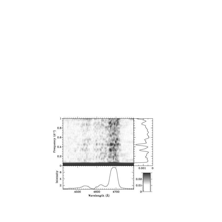
Figure 3: The pixel-to-pixel CLEANed PS of the rectified spectra of epoch I. The lower and right-hand panels show the mean spectrum and the normalized, integrated power over all pixels, respectively. The highest peak corresponds to a frequency: $\nu_{0}$ $\approx$ 0.444 d^-1. The gain and the number of iterations have been set to 0.3 and 250, respectively.

After demonstrating that the integrated properties of the line profile are periodic in nature, it is natural to ask whether the same recurrence timescale is present in the detailed LPVs. To this end, we performed pixel-to-pixel CLEANing of the epoch I and II data sets. All spectra were rebinned in a similar manner and were used as independent time sequences, thus creating 1024 CLEANed PS along the wavelength direction. This procedure confirms the presence of $\nu_{0}$, along with its first harmonic at $\nu_{1}$ $\approx$ 0.88 d^-1 over the entire line profile of He II $\lambda$4686 during epoch I, along with weak traces of this period in He II $\lambda$4542, N V $\lambda$$\lambda$4604, 4620 and N III $\lambda$4640 (Fig.3). As in the PS of the FWHM time series of epoch I (Fig.1), a periodic signal at $\nu_{2}$ $\approx$ 0.326 d^-1 is also present in the pixel-to-pixel CLEANed PS. The occurence of the same signal at $\nu_{2}$ in the FWHM and pixel-to-pixel CLEANed PS raises the possiblity that this feature is real. However, $\nu_{0}$ (or its harmonics) is generally (within the uncertainties) recovered in the epoch II PS, contrary to $\nu_{2}$. More importantly, the gray-scale plot of He II $\lambda$4686 does not show a coherent pattern of variability when folded with $\nu_{2}$, whereas it does when folded with $\nu_{0}$ (see below). Also, the phase diagram of the FWHM data of epoch I is considerably noisier when folded with this frequency. Further observations are essential to indicate whether this period is genuinely spurious. Although the LPVs of He II $\lambda$4686 for epoch II are undoubtedly periodic with a frequency of $\nu_{0}$ (see below), only a weak signal appears in the pixel-to-pixel PS at this frequency on the top of He II $\lambda$4542 and He II $\lambda$4686. This may be related to the more complex pattern of variability compared to epoch I.

The next analysis we have performed consisted in grouping the spectra for each epoch into 0.02 phase bins. The individual, binned He II $\lambda$4686 line profiles minus their corresponding unweighted means for each epoch are arranged as a function of phase in the upper panels of Figures 4a-4c. This line transition was chosen because its LPVs are quite representative of (but stronger and clearer than) that of the other He II spectral features ($\S$ 4.3). In view of the long time span of the observations (13, 4, and 63 cycles for epochs I, II, and III, respectively), He II $\lambda$4686 presents a remarkably coherent phase-related pattern of variability. However, it is noteworthy that significant cycle-to-cycle differences in the line-profile morphology are often found, a fact which is reflected in the gray-scale plots by discontinuities in the pattern of variability between consecutive bins (especially for epoch III; Fig.4c). Four main factors can induce this: (i) lack of long-term coherency in the pattern of variability; (ii) artificial loss of coherency induced by the uncertainty in the period; (iii) presence of additional small-scale profile variations created by shocked (and possibly turbulent) material carried out by the global stellar outflow, as observed in other WR stars (Lépine & Moffat 1999); and (iv) continuum flux variations for which no allowance has been made; we deem this last factor as a less important effect because of the small amplitude of the changes (see below). Concerning the first two points, note that the smaller the time span of the observations (Table 1), the higher the coherency.

4.1.2 Photometry

For the analysis of the broadband photometry, we only use the $V$-filter data as being less contaminated by emission lines (about 7 % of the total $V$ flux), along with all available mediumband visual-filter photometry, in total 734 observations binned to 0.1 day (1 day for the $HIPPARCOS$ data). Note that for WR 134, the small-scale variations observed in $U$, $B$, and $V$ are fairly well-correlated in general (Moffat & Marchenko 1993b).

Combining all 1989-1997 data and reducing them to the APT photometric system, we concentrate on a search for relatively short periods; a detailed investigation of the temporal behavior of the “secular” components (i.e., $\cal P$ $\approx$ 625 day and $\cal P$ $\approx$ 40 day variations) being presented in Marchenko et al. (1996b) and Marchenko & Moffat (1998a).

We constructed a CLEANed PS of the whole photometric data set, but failed to find any significant peaks in the range of interest, i.e., around the expected 2.3 day component. This is possibly due to the lack of coherency of the period on long timescales. The long-term component with $\cal P$ $\approx$ 625 day completely dominates the PS, followed by a less evident power peak at $\cal P$ $\approx$ 40 day. Pre-whitening from both long-period variations does not improve the situation in the high-frequency domain.

In the analysis of the data subsets, we have encountered some limited success. The “subsets” are naturally-imposed segments (e.g., summer monsoon and winter gaps at the APT, short-term campaigns of intense monitoring), with gaps between the segments exceeding, or comparable to, the length of the segment filled by observations. We obtain 14 such segments, covering the period HJD 2,447,859-2,450,636, with the number of observations per segment varying from 9 to 161. The most frequently appearing detail in the CLEANed PS is clustered around $\nu$ = 1.3-1.4 d^-1 (in 5 out of 14 PS). Twice, we detect a fairly strong signal at $\nu$ $\approx$ 0.9 d^-1: HJD 2,448,896-2,448,976 (43 observations), and HJD 2,450,522-2,450,636 (82 observations). Concerning the most abundant data set secured during the 1992 campaign (161 data points distributed over 135 days; practically all of them are shown on Fig.5), the expected signal at $\nu_{0}$ = 0.440 $\pm$ 0.018 d^-1 is enhanced only during a few cycles, between HJD 2,448,818-2,448,824 (Fig.5). We have used the data shown in the middle section of Figure 5 to construct a folded light curve with $\cal P$ = 2.27 day (ephemeris from McCandliss et al. 1994). Despite the fact that the periodic signal found during the interval HJD 2,448,818-2,448,824 is identical to the one found in the independently and practically simultaneously acquired spectroscopic data set — thus demonstrating that this detection is unlikely to be fortuitous —, the very noisy appearance of the folded light curve (Fig.6) shows that the detection of the $\cal P$ = 2.27 day periodicity is only marginal in the photometric data set. Adopting $\nu_{0}$ $\approx$ 0.44 d^-1 as the principal frequency, we may interpret the $\nu$ $\approx$ 0.9 and 1.3-1.4 d^-1 components found in the other subsets as the first and second harmonics, respectively.

Another intensive multi-site monitoring campaign in 1995 reveals the presence of the long-term $\cal P$ $\approx$ 40 day cyclic component (Marchenko et al. 1996b, and our Fig.7), masking the relatively weaker $\nu_{1}$ $\approx$ 0.88 d^-1 frequency, along with the possible initiation of $\cal P$ $\approx$ 7-8 day variations (perhaps as in Antokhin & Cherepashchuk 1984) at HJD 2,449,920-2,449,948. The latter phenomenon points to the transient character of the $\cal P$ $\approx$ 7-8 day variations.

4.2 Similarities of the Variations Across a Given Line Profile

In an attempt to objectively and quantitatively examine a potential relationship in the pattern of variability displayed by different portions of a given line profile, we have calculated the Spearman rank-order correlation matrices (see, e.g., Johns & Basri 1995; Lago & Gameiro 1998) whose elements $r(i,j)$ give the degree of correlation between the line intensity variations at any pixels $i$ and $j$ across the line profile (these matrices are symmetric and a perfect positive correlation is found along the main diagonal where $i$ = $j$). These matrices for He II $\lambda$4686 are shown for all epochs in Figure 8, in the form of contour plots, where the lowest contour indicates a significant positive or negative correlation at the 99.9 % confidence level.

An inspection of these matrices allows one to draw the following general conclusions: (i) There are various regions in the auto-correlation matrices presenting a significant positive or negative correlation; (ii) If the variations were principally induced by the changes in the continuum flux level ($\S$ 4.1.2), one would observe a tendency for a positive correlation over a substantial fraction of velocity space; this is clearly not observed; (iii) The main diagonal is not a straight line with a width corresponding to the velocity resolution (at most 100 km s^-1 in our case), as expected if two contiguous velocity elements would vary in a completely uncorrelated fashion, but is considerably wider. This suggests that the same pattern of variability affects simultaneously a fairly large velocity range of the profile, as independently found by Lépine, Moffat, & Henriksen (1996), who derived a relatively large mean line-of-sight velocity dispersion for the emission subpeaks travelling across the line profile of WR 134 ($\overline{\sigma_{\xi}}$ $\approx$ 440 km s^-1) compared to other WR stars in their sample ($\overline{\sigma_{\xi}}$ $\approx$ 100 km s^-1).

If we turn to a detailed epoch-to-epoch comparison of the matrices in Figure 8, we find significant differences (note that the phase coverage is sufficiently similar for all epochs for a direct comparison to be made). For example, a positive correlation is observed for epoch I at (– 500, + 2400) and (+ 200, + 1800) km s^-1, whereas the variations in these velocity ranges are rather negatively correlated for epoch II. The paucity of contours for epoch III indicates that no significant relationship existed for this epoch between the changes presented by different portions of the He II $\lambda$4686 line profile. This leads to the conclusion that the global pattern of variability is likely to differ notably in nature on a yearly timescale, although the LPVs are coherent over shorter timescales when phased with the 2.27 day period (Figs.4a-4c).

4.3 Similarities Between the Variations of Different Lines

The similar qualitative behavior of different lines has already been emphasized in the past (McCandliss 1988; Marchenko 1988; Vreux et al. 1992; McCandliss et al. 1994). Here, we re-address this point by calculating the degree of correlation between the LPVs at different projected velocities (referred to the line laboratory rest wavelength) in two given line profiles. The spectra obtained during epoch III are well suited for this purpose because of their wide spectral coverage. The correlation matrices of He II $\lambda$5412 with He II $\lambda$4542, He II $\lambda$4686, He II $\lambda$4859, and the doublet C IV $\lambda$5806 are presented for this epoch in Figure 9. As revealed by the prevalence of contours along the main diagonal, the LPVs presented by the He II lines are generally well correlated (this is especially true for the relatively unblended lines He II $\lambda$5412 and He II $\lambda$4686), emphasizing that they vary in a fairly similar fashion. This is remarkable as the presence of blends and/or noise tends to mask any potential correlation. Only the blue wings of He II $\lambda$5412 and C IV $\lambda$5806 are positively correlated for epoch III. The changes affecting He II $\lambda$4686 and He II $\lambda$4542 are also well correlated for epochs I and II.

5 Discussion

5.1 The Duplicity of WR 134 Questioned

In view of the long-suspected association of WR 134 with an orbiting collapsed companion (Antokhin et al. 1982; Antokhin & Cherepashchuk 1984), we discuss below the implications of these observations with respect to this scenario.

5.1.1 The Expected Emergent X-ray Luminosity

An interesting issue is whether the predicted X-ray luminosity produced by the accretion process (after allowance for wind absorption) can be reconciled with the X-ray observations of WR 134.

First, if we associate the 2.27 day periodicity with orbital motion, we can obtain an estimate of the location of the compact object in the WR wind. Assuming for simplicity a circular orbit (i.e., that the circularization timescale is shorter than the evolutionary timescale; Tassoul 1990), a canonical mass for the secondary as a neutron star, $M_{X}$ = 1.4 M_⊙, and a mass for WR 134, $M_{\star}$ = 11 M_⊙ (Hamann, Koesterke, & Wessolowski 1995), we obtain an orbital separation of $a$ $\approx$ 17 R_⊙, or $a$ $\approx$ 6 WR core radii (Hamann et al. 1995).

Second, the total X-ray luminosity (in ergs s^-1) produced by Bondi-Hoyle accretion of a stellar wind onto a degenerate object can be expressed by the following relation (Stevens & Willis 1988):

$$L_{X}\approx 2.03\times 10^{57}\>\eta\>\dot{M}\>M_{X}^{2}\>a^{-2}\>v(a)^{-4}\left(1-\frac{L_{X}}{L_{E}}\right)^{2},$$ (1)

where $\eta$ is the efficiency of the conversion of gravitational energy into X-ray emission; $\dot{M}$ the mass-loss rate of the primary (in M_⊙ yr^-1); $v(a)$ the WR wind velocity at the secondary’s location (in km s^-1), and $L_{E}$ the Eddington luminosity (in ergs s^-1) given by $L_{E}\approx 5.02\times 10^{37}M_{X}/\sigma_{e}$ (the electron scattering coefficient $\sigma_{e}$ = 0.35). In this expression, we neglect the orbital velocity of the secondary relative to the (much larger) WR wind velocity. For the latter, we start by arbitrarily adopting the well-established mean velocity law for O stars of the form (Pauldrach, Puls, & Kudritzki 1986):

$$v(r)=v_{\infty}\>(1-R_{\star}/r)^{0.8}.$$ (2)

Note that at the assumed location of the secondary ($r$ $\approx$ 6 $R_{\star}$; see above) the wind has almost reached its terminal velocity, $v_{\infty}$ = 1900 km s^-1 (Rochowicz & Niedzielski 1995). We further assume: $\dot{M}$ = 8 $\times$ 10^-5 M_⊙ yr^-1 (Hogg 1989), and $\eta$ = 0.1 (McCray 1977). This yields: $L_{X}$ $\approx$ 1.4 $\times$ 10³⁷ ergs s^-1.

We have modeled the emergent X-ray flux by a power law with energy index $\alpha$, substituted above a characteristic high-energy cutoff $E_{c}$ by the function $\exp[(E_{c}-E)/E_{f}]$, as commonly observed in accretion powered pulsars (White, Swank, & Holt 1983; Kretschmar et al. 1997). The values of $\alpha$, $E_{c}$, and $E_{f}$ are chosen to be roughly representative of accreting pulsars: $\alpha$ $\approx$ – 0.2; $E_{c}$ $\approx$ 15 keV; $E_{f}$ $\approx$ 15 keV (White et al. 1983). The X-ray spectrum was normalized to the total X-ray luminosity determined above, i.e., $L_{X}$ = 1.4 $\times$ 10³⁷ ergs s^-1.

The next step is to evaluate the attenuation of the beam of photons as they propagate through the stellar wind. Since the absorption properties of ionized plasmas are dramatically dependent on their ionization state (e.g., Woo et al. 1995), one has first to determine to what degree the accreting compact object ionizes the surrounding stellar wind. The presence of an immersed, strongly ionizing companion is expected to create an extended X-ray photoionized zone in its vicinity (Hatchett & McCray 1977). An investigation of the effect of the ionizing X-ray flux coming from the secondary on the surrounding wind material requires a detailed calculation of the radiative transfer (Kallman & McCray 1982). However, good insight into the ionization state of an optically thin gas illuminated by a X-ray point source can be obtained by considering the quantity (Hatchett & McCray 1977):

$$\xi(r,r_{X})=\frac{L_{X}}{n(r)r_{X}^{2}}=\frac{4\pi L_{X}\overline{m}}{\dot{M}}\>v(r)\left(\frac{r}{r_{X}}\right)^{2},$$ (3)

with: $n(r)$ the local number density of the gas; $r_{X}$ the distance from the X-ray source. This expression is derived using the mass continuity equation: $\dot{M}$ = 4 $\pi$ $r^{2}$ $\overline{m}$ $n(r)$ $v(r)$. Here, $\overline{m}$ is the average mass per ion (we assume a pure helium atmosphere). The velocity of the material as a function of $r$ is given by equation (2). The variations of $\log\xi(r,r_{X})$ are illustrated as viewed from above the orbital plane in Figure 10. In the limit $\xi\rightarrow 0$ ergs cm s^-1, the ionization balance of the material is unaffected by the presence of the X-ray emitter, i.e., is principally governed by the radiation field of the WR star. We stress that this model assumes an optically thin plasma. In reality, the mean path length of the X-ray photons is considerably shorter, and it is thus likely that the X-ray photoionized zone would be dramatically less extended — especially in the direction toward the primary — than sketched here.

The predicted (after wind absorption) X-ray luminosities for the wavebands corresponding to the $PSPC$ and $IPC$ detectors onboard the ROSAT and Einstein observatories (0.2-2.4 and 0.2-4.0 keV, respectively) have been computed for three illustrative cases spanning a wide range in the wind ionization state, namely $\log\xi$ = 2.1, 1.8, and 0 ergs cm s^-1. The photoelectric atomic cross sections for ionized plasmas are taken from Woo et al. (1995). Thompson scattering by the free electrons was also taken into account. The two former values, $\log\xi$ = 2.1 and 1.8 ergs cm s^-1, are roughly what would be expected in the framework of our model (Fig.10), whereas in the latter case, $\log\xi$ = 0 ergs cm s^-1, we explore the (somewhat unrealistic) case in which the presence of the neutron star has no effect on the surrounding stellar wind. In this case, photoelectric cross sections for cold interstellar gas were used (Morrison & McCammon 1983). Because the WR wind material is, by nature, far from neutral, the derived X-ray luminosities are here strictly lower limits.

Pollock (1987) reported on two pointed IPC observations of WR 134 obtained with the Einstein satellite, with no evidence for variability (see his Table 5). The derived (corrected for interstellar extinction) X-ray luminosity in the 0.2-4.0 keV band, 4.6 $\pm$ 1.6 $\times$ 10³² ergs s^-1, being consistent with the upper limit derived by Sanders et al. (1985): 4.5 $\times$ 10³² ergs s^-1 (when scaled to the same adopted distance of 2.1 kpc; van der Hucht et al. 1988). On the other hand, a single measurement (due to the ROSAT satellite) is available in the 0.2-2.4 keV range (Pollock, Haberl, & Corcoran 1995). With no clear indication of X-ray variability, we will assume in the following that the typical observed (and corrected for interstellar extinction) X-ray luminosities from WR 134 are: 0.46 $\pm$ 0.22 and 4.6 $\pm$ 1.6 $\times$ 10³² ergs s^-1 in the 0.2-2.4 and 0.2-4.0 keV bands, respectively.

These values can be directly compared with the predicted X-ray luminosities after wind absorption shown as a function of orbital phase in Figure 11. For $\log\xi$ = 2.1 and 1.8 ergs cm s^-1, the observed luminosities are systematically much lower than expected in the framework of our model, with a deficiency reaching 2-3 orders of magnitude. For $\log\xi$ = 0 ergs cm s^-1, the ROSAT data are consistent with the expectations. However, and unless the Einstein satellite observed WR 134 near X-ray eclipse, the same conclusion does not hold for the data in the 0.2-4.0 keV band, with an order of magnitude deficiency. Although mildly significant, this deficiency shows that, even in the extreme case in which the presence of the accreting neutron star has a negligible effect on the WR wind, the observed and predicted X-ray luminosities can hardly be reconciled. Overall, and although we stress that more detailed and rigorous calculations are necessary, the deficiency of the observed X-ray flux must thus be regarded as serious. This conclusion is bolstered if one considers that wind radiative instabilities may largely account for the observed fluxes (typically 10^32-33 ergs s^-1 in the 0.2-2.4 keV range; Wessolowski 1996).

Assuming a lower mass-loss rate due to clumping (Moffat & Robert 1994; Nugis, Crowther, & Willis 1998) may, at best, reduce the discrepancy by one order of magnitude (see equation [1]). In contrast, however, assuming a “softer” $v(r)$ law (i.e., $\beta$ $>$ 0.8; see equation [2]) for WR stars (Schmutz 1997; Lépine & Moffat 1999; Antokhin, Cherepashchuk, & Yagola 1998), or taking into account the existence of a velocity plateau inside the photoionized zone (Blondin 1994), exacerbates the discrepancy.

Considering that the soft X-ray flux of WR 134 is very similar to that of other bona fide single WN stars (Pollock 1987), and was even among the lowest found for single WN 6 stars during the ROSAT all-sky survey (Pollock et al. 1995), this deficiency of predicted X-ray flux suggests centrifugal (or magnetic) inhibition to prevent the gravitational capture by the compact object of the primary’s wind material (the so-called “propeller effect”; Lipunov 1982; Campana 1997; Cui 1997; Zhang, Yu, & Zhang 1998). Note that orders of magnitude deficiency in the X-ray flux is observed in some high-mass X-ray binaries (HMXRBs; e.g., Taylor et al. 1996).

5.1.2 Modeling the Line-Profile Variations Caused by an Ionizing X-ray Source

Keeping in mind that the accretion process would be, as suggested above, much less efficient than expected in the Bondi-Hoyle approximation — and therefore that the influence of the X-ray source on the surrounding wind material would be far less severe than sketched in Figure 10 — we performed simulations of the LPVs caused by the orbital revolution of a localized, strongly ionized wind cavity.

We proceed with numerical simulations of the observed LPVs of the representative He II $\lambda$4686 line, binning the epoch I spectra to 0.1 phase resolution. We modify the SEI code (Sobolev method with exact integration: Lamers, Cerruti-Sola, & Perinotto 1987; hereafter LCP) to allow for the variation of the source function in a 3-D space, thus breaking the initially assumed spherical symmetry of the WR wind. The variation of the unperturbed source function as a function of the radial distance from the star is described by equation (4) of LCP. The wind dynamics is assumed to be identical inside, and outside the photoionized cavity. Specifically, we adopt a $\beta$-velocity law with an exponent $\beta$ = 3 and a ratio of the wind velocity at the inner boundary of the optically thin part of the WR wind to the terminal velocity, $w_{0}$, of 0.25 (see equation [35] of LCP).

We start from the assumption that the underlying, unperturbed line profile is not affected by any phase-dependent variations. We fit this reference profile with the standard SEI code, preserving complete spherical symmetry. Throughout these simulations, we adopt $\tau_{T}$ = 0.60, $\alpha_{1}$ = 6.0, $\alpha_{2}$ = 0.5, $\epsilon_{0}^{\prime}$ = 12.0, $B_{0}$ = 1.2, $a_{T}$ = 0.2, and $w_{D}$ = 0.25 (these values are uncertain to about 30 %). We refer the reader to LCP for a complete description of these parameters. Note that these values slightly differ from those adopted by Marchenko & Moffat (1998b) due to a different approach in modelling (adopting their values, however, would not qualitatively modify the conclusions drawn in the following). Note that while the issue of the flattened, asymmetric wind in WR 134 is appealing (Schulte-Ladbeck et al. 1992; Moffat & Marchenko 1993b), this inevitably introduces a great and probably unnecessary complexity into the simulations.

There are two obvious choices for the reference profile of the unperturbed wind: a minimum-emission or maximum-emission profile, derived from a smoothed minimum/maximum emissivity at a given wavelength for a given phase (Fig.12). By introducing 3-D variations into the source function of the unperturbed wind corresponding to the minimum-emission reference profile, we immediately find that we are not able to reproduce the observed LPVs with any reasonable choice of the parameters. Thus we adopt the maximum-emission representation of the unperturbed profile as a starting approximation.

To simulate the X-ray induced cavity in the otherwise spherically symmetric wind, we require the following free parameters: $\Theta$ — the azimuthal extension of the cavity; $\Delta z$ = $\Delta p$ — line-of-sight and impact-parameter extension of the cavity; $\Delta z_{0}$ — line-of-sight distance of the cavity’s inner boundary from the stellar core; $i$ — orbital inclination; $k$ — coefficient describing the deviation of the source function within the cavity, namely $S(cavity)$ = $k$ $\times$ $S(wind)$; $\phi_{0}$ — cross-over phase (frontal passage of the cavity). We assume a circular orbit. A sketch of the adopted geometry is shown in Figure 13.

With these parameters, we attempt to fit all the phase-binned profiles, minimizing the observed minus model deviations in the $\chi^{2}$ sense, while reproducing the observed TVS of He II $\lambda$4686 (Fig.12). We also attempt to make the (O – C) profile deviations distributed as evenly as possible over the entire phase interval. We concentrate on the goodness of the fit for the velocities not exceeding $\pm$ 0.8 $v_{\infty}$, since it is impossible to match the red wing of the He II $\lambda$4686 profile (electron scattering effect; see Hillier 1991) as well as the bluemost portion (partial blending with N III transitions).

After an extensive search for optimal parameters, we find that the following set reproduces the observed LPVs reasonably well (Fig.14): $\Theta$ = 140 $\pm$ 10^∘, $\Delta z$ = $\Delta p$ = 8 $\pm$ 0.5 $R_{\star}$, $\Delta z_{0}$ = 2.7 $\pm$ 0.2 $R_{\star}$, $i$ = 65 $\pm$ 5^∘, $k$ = 0.07 $\pm$ 0.01 (i.e., practically zero emissivity from the X-ray eroded wind), and $\phi_{0}$ = 0.55 $\pm$ 0.03. This value of $\phi_{0}$ means that the X-ray source passes in front when the continuum flux undergoes a shallow minimum (Fig.6). The largest (O – C) deviations are concentrated around phases 0.0 and 0.5. By no means are we able to reproduce the extended emissivity excesses at $v$ $\approx$ – 0.5 $v_{\infty}$ ($\phi$ = 0.35) and $v$ = + (0.5-0.7) $v_{\infty}$ ($\phi$ = 0.65 and 0.75). These deviations might be generated by a low-amplitude velocity shift of the underlying profile as a whole, due to binary motion (partially inducing the centroid variations seen in Fig.2). We will not consider this possibility further, as it will add more free parameters into the model. We are able to reproduce only the general appearance of the TVS as a structured, non-monotonic function with 3 distinct maxima, without precise match of their amplitudes and positions (Fig.12).

According to Model 5 of Kallman & McCray (1982), helium is fully ionized for $\log\xi$ $\ga$ 1.5 ergs cm s^-1. The derived azimuthal and radial extensions of the cavity indeed match fairly well the size of the highly ionized zone with $\log\xi$ $\approx$ 1.5 ergs cm s^-1 (Fig.10), especially if we take into account its large azimuthal extension. However, since the accretion is likely to be partially inhibited and the WR wind is not optically thin, the real photoionized cavity will be much less extended than sketched in Figure 10. For example, reduction of the efficiency of the X-ray generation by 1-2 orders of magnitude would dramatically reduce the dimension of the $\log\xi$ $\approx$ 1.5 cavity (to the size of the $\log\xi$ $\ga$ 2.5 cavities sketched in Figure 10; see equation [3]). The local nature of this putative zone is also suggested by an inspection of the P Cygni absorption profile variations of He I $\lambda$4471 and N V $\lambda$4604. The epoch I spectra have been groupped into broad phase bins of width 0.2 (the P Cygni absorptions are very weak, thus requiring an extremely high S/N), and are overplotted in Figure 15. It is apparent that potential phase-related variations do not significantly exceed the observationally-inflicted accuracy. Thus, neither the base of the wind (N V $\lambda$4604), nor the relatively distant regions (He I $\lambda$4471) are seriously affected by the presence of the photoionized cavity. An inspection of 16 archive IUE SWP spectra of WR 134 obtained during the period 1989 November 30 - December 6 (see Table 3) also shows that no UV lines with well-developed P Cygni absorption components show any significant variability in their absorption troughs. Hints of relatively weak, possibly phase-locked variations are only evident in the emission parts.

We conclude that despite the encouraging similarity between the observed and modeled line-profiles, the relatively large derived size of the cavity ($R$ $\approx$ 8 $R_{\star}$) along with its large azimuthal extension seem to enter in conflict with the low level of X-ray flux observed from WR 134.

5.1.3 On the Origin of the Long-Term Modulations

Another question we may ask is whether this model is able to account for the $\cal P$ $\approx$ 40 and $\cal P$ $\approx$ 625 day recurrence timescales present in the photometric data (Marchenko et al. 1996b; Marchenko & Moffat 1998a), as well as the epoch-dependent nature of the LPVs (Figs.2 and 4).

As the wind approaches the compact object, it is gravitationally focused, forming a standing bow shock. This leads to the formation of an extended wake downstream (Blondin et al. 1990). This process is suspected to be non-stationary in HMXRBs, with the possible formation of a quasi-cyclical “flip-flop” instability (Benensohn, Lamb, & Taam 1997; but see Ruffert 1997), with characteristic timescales comparable to the flow time across the accretion zone ($\approx$ minutes); too short a timescale to account for any observed long-term variations in WR 134.

Alternatively, it is tempting to associate the 40 day recurrence timescale to the precession of a tilted accretion disk as suggested in some HMXRBs (Heermskerk & van Paradijs 1989; Wijnands, Kuulkers, & Smale 1996). The condition for the creation of a persistent accretion disk around a wind-fed neutron star orbiting an early-type companion can be written as (Shapiro & Lightman 1976):

$$2.7\times 10^{-11}\gamma^{8}B_{12}^{-4/7}R_{10}^{-10/7}M_{X}^{20/7}M_{\star}^{-4}P^{-2}R_{\star}^{4}L_{X}^{2/7}\ga 1$$ (4)

With $B_{12}$ the surface magnetic field of the neutron star in units of 10¹² Gauss, $R_{10}$ the radius of the neutron star in units of 10 km, $M_{X}$ and $M_{\star}$ in units of solar masses, $P$ in units of days, $R_{\star}$ in units of solar radii, and $L_{X}$ in units of ergs s^-1. $\gamma$ is expressed by the relation: $\gamma\approx\zeta^{1/2}\left[v_{esc}/v(a)\right]$ where $\zeta$ is a dimensionless quantity accounting for the deviation from the Hoyle-Lyttleton treatment, and $v_{esc}$ the escape velocity at the WR “photosphere” (we neglect the orbital velocity of the neutron star relative to the WR wind velocity). Taking $B_{12}$ = $R_{10}$ = $\zeta$ = 1, we obtain a value much below unity ($\sim$ 10^-4), suggesting that accretion mediated by a persistent disk in WR 134 would be very unlikely.

A viable mechanism that might, however, account for the  monthly changes in the spectroscopic pattern of variability (Figs.2 and 4) is to consider long-term changes in the accretion rate (thus varying the size of the ionized cavity surrounding the compact companion).

5.2 Wind-Related Variability?

Although the encouraging agreement between the observed and modeled LPVs (Fig.14) leads to the conclusion that the model involving an accreting compact companion cannot be completely ruled out by the present observations, the very low observed X-ray flux of WR 134 which imposes inhibited accretion, as well as the long-term changes in the accretion rate required to account for the epoch-dependent nature of the LPVs, set serious constraints on this model. This, together with the inconclusive search for rapid periodic photometric variations, possibly induced by a spinning neutron star (Antokhin et al. 1982; Marchenko et al. 1994) can be used to argue that the existence of such a low-mass collapsed companion is questionable.

Alternatively, it is conceivable that we observe rotationally-modulated variability in WR 134. Indeed, the global pattern of spectral variability resembles in some aspects that of the apparently single WR star EZ CMa, for which the existence of a rotation-modulated, structured wind has been proposed (St-Louis et al. 1995; Morel et al. 1997, 1998; Harries et al. 1999). By analogy with EZ CMa, the He II line profiles vary in a fairly similar fashion (Vreux et al. 1992, and our Fig.9), changes in line skewness or FWHM generally demonstrate a rather simple and well-defined behavior when phased with the 2.27 day period (Fig.2), and a positive/negative correlation between the pattern of variability presented by different parts of the same line profile is occasionally found (Fig.8). Other outstanding properties shared by WR 134 and EZ CMa are the epoch-dependent nature of the variations, as well as the substantial depolarization of the emission lines (Harries et al. 1998); this last point being generally attributed to an equatorial density enhancement (see also Ignace et al. 1998).

Another piece of evidence pointing to the similarity between WR 134 and EZ CMa comes from the broadband ($\sim$ continuum) polarimetric observations of Robert et al. (1989). Plots of the Stokes parameters $Q$ and $U$ of WR 134 versus phase are shown in Figure 16 (because of a likely loss of coherency over long timescales, the two data subsets separated by a year are plotted separately). The data show strong epoch-dependent variations, with a clear single-wave variation in $U$ (less clear in $Q$) in 1985, and a fairly clear double-wave modulation in $Q$ (less clear in $U$) in 1986. This behavior is qualitatively very similar to what is observed in EZ CMa (e.g., Robert et al. 1992), although the polarimetric variations are not as clearly phase-locked in WR 134. Such a drastic change from a single-wave to a double-wave modulation in data taken one year apart is not easily acommodated by a binary hypothesis. However, neither the amount, nor the time coverage of the polarimetric data allow to regard it as a decisive evidence favoring the single-star interpretation. Although the 7 nights of linear spectropolarimetry of WR 134 by Schulte-Ladbeck et al. (1992) do show variations, both in the continuum and in the lines, the data are sparsely spread out over 6 months, making it impossible to separate variations on the 2.3-day cycle from long-term epoch-dependent variations. Certainly, further more intense spectropolarimetry on different timescales in all 4 Stokes’ parameters will prove quite interesting.

Relying on the EZ CMa and WR 134 similarities, one may speculate that the 2.3 day periodicity in WR 134 is induced by a small number of spatially extended, relatively long-living and rotating wind streams whose formation is possibly triggered by photospheric perturbations, such as magnetic structures or pulsations (e.g., Cranmer & Owocki 1996; Kaper et al. 1997). Contrary to EZ CMa, however, WR 134 does not show any detectable phase-related changes in the UV or optical P Cygni absorption troughs, nor a clear correlation between changes occuring near the hydrostatic stellar “surface” and in the wind.

By speculating about the existence of (non)radial pulsations in WR 134 (although a search for related rapid light variations has been hitherto inconclusive; Cherepashchuk 1975; Antokhin et al. 1992), and exploring the idea of interactions between different pulsational modes, one is led to the notion of quasi-periodic ejection of shell-like structures. This idea can be explored via the application of the model introduced above for the anisotropic wind ($\S$ 5.1.2). We allow for the formation of a shell with enhanced optical depth in the otherwise spherically symmetric wind. The shell geometry may be variable but, for the sake of simplicity, we mainly explore the spherically symmetric case. The shell can slowly propagate outwards at a given rate, slightly expanding and gradually approaching the physical conditions in the unperturbed surrounding wind. Indeed, at least the variations in the blue wing of He II $\lambda$4686 (Figs.4a and 14) somewhat mimic the expected behavior of such an outwardly-moving structure. However, there is also pronounced asymmetry between the blue and red parts of the He II $\lambda$4686 profile, especially obvious around $\phi$ = 0.35-0.55 (Fig.14). This asymmetry cannot be reproduced by any adjustment of the model free parameters, unless one makes the contrived assumption that the front- and back-side lobes of the shell are formed under different physical conditions. This leads us to discard the model of an expanding shell with central symmetry.

Although the existence of a globally inhomogeneous outflow in WR 134 is attractive, such an interpretation is also not without difficulties. For instance, the origin of the long-term (quasi)periodic changes in continuum flux, and of the epoch-dependency of the spectral changes remains unexplained. Magnetic activity, by inducing long-term changes in the global wind structure, may constitute a convenient, although largely ad hoc, way to accomodate this aspect of the variability.

TABLE 1 – JOURNAL OF SPECTROSCOPIC OBSERVATIONS.

		HJD		Number	Spectral	Reciprocal Dispersion
Epoch	Date	– 2440000	Observatorya	of Spectra	Coverage (Å)	(Å  pix-1)	S/N
I	92 Jul - Aug	8813-8843	SPM	65	4380-4790	0.41	$\sim$ 160
II	93 Oct	9258-9269	SPM	38	3990-4840	0.83	$\sim$ 115
III	95 May - Oct	9860-10005	OMM, DAO	32	4360-5080	1.62	$\sim$ 210
				30	5050-5945	1.62	$\sim$ 290

^a SPM: San Pedro Mártir Observatory 2.1 m (Mexico); OMM: Observatoire du Mont Mégantic 1.6 m (Canada); DAO: Dominion Astrophysical Observatory 1.2 m (Canada).

TABLE 2 – JOURNAL OF PHOTOMETRIC OBSERVATIONS.

	HJD		Number of Binned	Mode of	Filter
Date	– 2440000	Observatorya	Observations	Observation	Setb
89 Nov - 93 Feb	7859-9045	HIPPARCOS	44	—	$Hp$ ($\sim$ $B$ + $V$)c
90 May - 97 Jul	8025-10636	APT	483	Diff. phot.	$V$
92 Jun - Jul	8800-8828	SPM	28	2-ch. phot.	5185 (250)
92 Jun - Jul	8800-8832	SPM	23	Diff. phot.	$V$
92 Jul	8819-8833	MO	55	Diff. phot.	6012 (87)
95 Jun - Jul	9885-9903	CR	13	Diff. phot.	$V$
95 Jun - Aug	9891-9949	SPM	88	Diff. phot.	$V$

^a APT: Automatic Photometric Telescope 0.25 m (USA); SPM: San Pedro Mártir Observatory 0.84 m (Mexico); MO: Maidanak Observatory 0.6 m (Uzbekistan); CR: Observational Station in Crimea 0.6 m (Ukraine).
^b For the midband filters, we provide the central wavelength and FWHM (in Å).
^c See van Leeuwen et al. (1997).

TABLE 3 – IUE SWP HIGH RESOLUTION SPECTRA OF WR 134.

SWP Image Number	JD – 2440000a	Phaseb
37705	7861.092	0.396
37707	7861.213	0.449
37718	7863.008	0.240
37725	7863.981	0.669
37727	7864.097	0.720
37734	7865.136	0.178
37735	7865.184	0.199
37737	7865.315	0.256
37739	7865.427	0.306
37741	7865.543	0.357
37743	7865.655	0.406
37745	7865.765	0.455
37748	7865.972	0.546
37750	7866.095	0.600
37755	7866.976	0.988
37757	7867.103	0.044

^a Julian Date at the midpoint of the exposure (2400 s for all spectra).
                                            ^b According to the ephemeris of McCandliss et al. (1994): $JD$ 2447015.753 + 2.27 $E$.

Figure 1: Power spectra (normalized to the total variance of the data) of the skewness, centroid, and FWHM time series of He II $\lambda$4686 for epoch I. Dotted line: raw PS; solid line: CLEANed PS. The short- and long-dashed horizontal lines indicate the 99.0 % and 99.9 % confidence levels for the presence of a deterministic signal in the time series, respectively. The number of iterations of the CLEAN algorithm, N, has been set to 3400 (skewness), 380 (centroid), and 4500 (FWHM); a gain g = 0.2 has been used throughout. The algorithm is generally insensitive to the combination of these two parameters in the range N $\ga$ 100 and g $\leq$ 0.5-0.8.

Figure 2: Skewness and centroid variations, deviations of the FWHM around the mean value (in km s^-1), and EW variations (normalized by division to the mean value) of He II $\lambda$4686 for each epoch, as a function of phase. The 2-$\sigma$ error bars for the EW values were calculated according to Chalabaev & Maillard (1983). As everywhere in this paper, the ephemeris of McCandliss et al. (1994) has been adopted: $HJD$ 2,447,015.753 + 2.27 $E$.

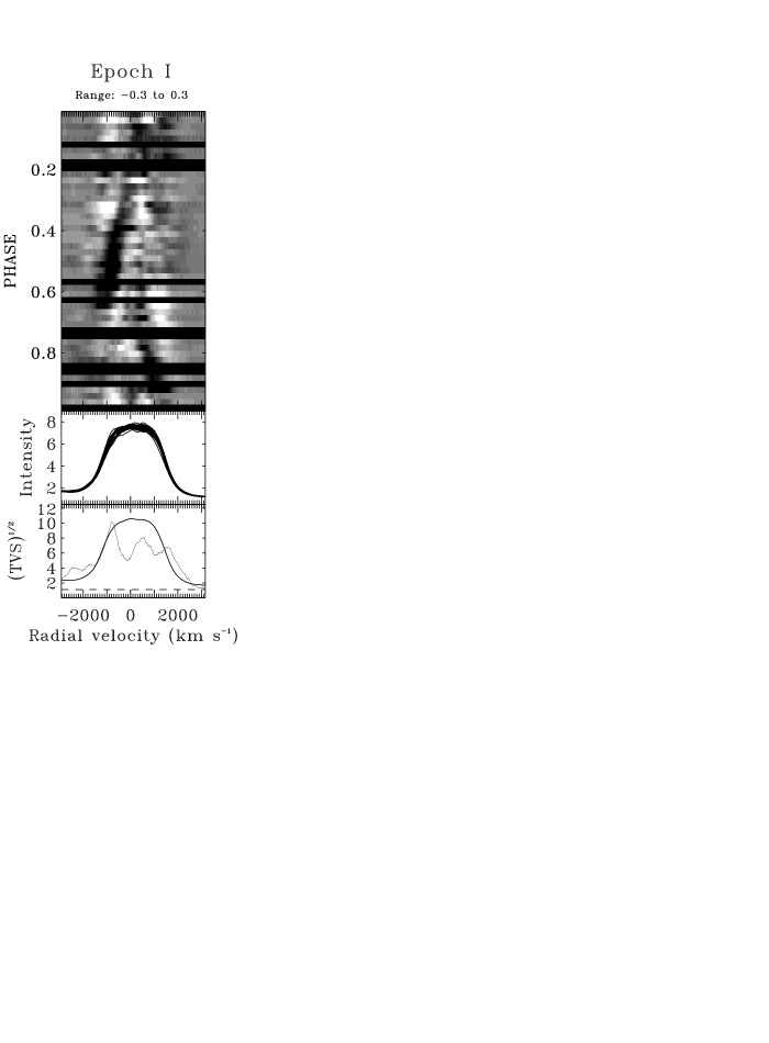
Figure 4: Gray-scale plots of the time series of the residuals of He II $\lambda$4686 for each epoch, as a function of phase. The residuals are the binned (to 0.02 phase resolution) He II $\lambda$4686 line profiles minus their corresponding unweighted means for each epoch. Excess emission components appear brighter in these plots. The middle portion of each panel shows a superposition of the rectified profiles. The values of the temporal variance spectrum (TVS; Fullerton, Gies, & Bolton 1996), along with the horizontal dashed line indicating the 99.0 % confidence level for significant variability, are displayed in the lower portion of each panel. The mean profile (in arbitrary units) of the epoch is overplotted. The gray-scales plots are displayed in the radial velocity frame (the radial velocities are referred to the line laboratory rest wavelength).

Figure 5: Photometry of WR 134 in 1992. Filled triangles: APT; open circles: SPM (Mexico) 1-channel photometry; filled circles: SPM 2-channel photometry; open triangles: Maidanak Observatory; open stars: $HIPPARCOS$. The bottom panel is an enlargement of the insert in the central panel. The sizes of the symbols correspond to 2-$\sigma$ error bars. In order to guide the eye in the bottom frame, a sinusoid with a period of 2.27 days (ephemeris of McCandliss et al. 1994) has been overplotted.

Figure 6: Photometry of WR 134 in 1992, folded with the $\cal P$ = 2.27 day period. Only the data plotted in the middle panel of Figure 5 have been used. The symbols are coded as in Figure 5.

Figure 7: Photometry of WR 134 in 1995. Filled triangles: APT; filled circles: SPM (Mexico); open triangles: Crimean Observational Station. The sizes of the symbols correspond to 2-$\sigma$ error bars.

Figure 8: Auto-correlation matrices of He II $\lambda$4686 for each epoch. Thick and thin contours indicate a negative or positive correlation in the pattern of variability presented by the same line profile at different radial velocities, respectively. The lowest contour is drawn for a significant correlation at the 99.9 % confidence level.

Figure 9: Correlation matrices of He II $\lambda$5412 with He II $\lambda$4542, He II $\lambda$4686, He II $\lambda$4859, and C IV $\lambda$5806 for epoch III. Thick and thin contours indicate a negative or positive correlation in the pattern of variability presented by two line profiles at different radial velocities (referred to the line laboratory rest wavelength), respectively. The lowest contour is drawn for a significant correlation at the 99.9 % confidence level.

Figure 10: Contours of constant ionization parameter $\log\xi$ (in ergs cm s^-1). The accreting, strongly ionizing compact companion is located at (0, 17). The WR star is placed at the origin of this plot.

Figure 11: Upper and middle panels: predicted X-ray luminosities after allowance for wind absorption in the 0.2-2.4 and 0.2-4.0 keV bands as a function of the orbital phase $\phi$, and for different values of the ionization parameter $\xi$: $\log\xi$ = 2.1 ergs cm s^-1 (solid line), $\log\xi$ = 1.8 ergs cm s^-1 (short-dashed line), and $\log\xi$ = 0 ergs cm s^-1 (long-dashed line). The shaded aeras show the range of the ROSAT and Einstein count rates for WR 134, namely 0.46 $\pm$ 0.22 and 4.6 $\pm$ 1.6 $\times$ 10³² ergs s^-1 in the 0.2-2.4 and 0.2-4.0 keV bands, respectively (Pollock, Haberl, & Corcoran 1995; Pollock 1987). The luminosities have been scaled to a distance of 2.1 kpc (van der Hucht et al. 1988). Note that the calculations do not consider the X-ray emission intrinsic to the WR wind (generally ascribed to radiative instabilities), nor the scattering of the neutron star emission in the WR wind which may cause extra emission at X-ray eclipse. Lower panel: column density of the absorbing wind material in units of 10²³ cm^-2, as a function of $\phi$.

Figure 12: Upper panel: solid line — the observed TVS; dotted line — the modeled TVS within the maximum-emission approach. Lower panel: solid line — mean epoch I profile of He II $\lambda$4686; dotted line — the SEI model fit within the maximum-emission approach; dashed line — the SEI model fit applying the minimum-emission approach. Note that the model is unable to fit the bluemost and redmost parts of the line profile because of partial blending and electron scattering effect, respectively. The projected velocity, w, is normalized to $v_{\infty}$ = 1900 km s^-1.

Figure 13: Sketch of the geometry adopted for the photoionization cavity. The azimuthal extension of the cavity, $\Theta$, is in the direction perpendicular to the plane of the figure.

Figure 14: The observed (solid line) and modeled (dotted line) phase-dependent variations of He II $\lambda$4686. All epoch I spectra are binned to 0.1 phase resolution; the bin mid-phase is shown in each panel.

Figure 15: Variations of the P Cygni absorption troughs of He I $\lambda$4471 and N V $\lambda$4604 with phase. All epoch I observations are binned to 0.2 phase resolution: dashed-dotted line: $\phi$ = 0.15-0.35; long-dashed line: $\phi$ = 0.35-0.55; short-dashed line: $\phi$ = 0.55-0.75; dotted line: $\phi$ = 0.75-0.95; solid line: $\phi$ = 0.95-1.15. Note that the intensity scale is different for the two panels.

Figure 16: The Stokes parameters $Q$ and $U$ of WR 134 in 1985-1986 (Robert et al. 1989) plotted in phase according to the ephemeris of McCandliss et al. (1994). Left and right panels: data (with 2-$\sigma$ error bars) for the intervals HJD 2,446,362-2,446,371 (1985) and HJD 2,446,704-2,446,735 (1986), respectively.