Evolution of supernova remnants in the interstellar medium with a large-scale density gradient

Abstract

The large-scale gradient of the interstellar medium (ISM) density distribution essentially affects the evolution of Supernova remnants (SNRs). In a non-uniform ISM, the shape of SNR becomes essentially non-spherical, and distributions of gas parameters inside the remnant become strongly anisotropic. The well-known self-similar Sedov solutions may not be applied to modelling such non-spherical objects. Therefore we propose a new approximate analytical method for full hydrodynamical description of 3D point-like explosions in non-uniform media with arbitrary density distribution.

On the basis of this method, we investigate the general properties of evolution of 2D non-spherical adiabatic SNRs in ISM with large-scale density gradient.

It is shown that the real shape of adiabatic SNR becomes more non-spherical with age, but the visible shape remains close to spherical even for strong real asymmetry (ratio of maximal to minimal shock radii) and surface brightness contrast. It is shown also that the values of the parameters of X-ray radiation from the entire SNR (luminosity, spectral index) are close to those in the Sedov case with the same initial data. However, the surface distribution of the X-ray emission parameters is very sensitive to the initial density distribution around the SN progenitor. Therefore, the X-ray maps give important information about physical conditions inside and outside of the non-spherical SNR.

1 Introduction

The investigation of Supernova remnants (SNRs) gives important information on the physics of Supernova (SN) explosions, on the properties of the surrounding interstellar medium (ISM) and on shock wave physics. The majority of galactic SNRs are in the adiabatic stage of evolution (Lozinskaya [1992]). If the density of the ISM is uniform, their hydrodynamics are well described by the self-similar Sedov solution (Sedov [1959], Shklovskiy [1962]). The typical values of plasma temperatures in SNRs are $T\simeq 10^{6}$ to $10^{8}\ {\rm K}$ and, therefore, SNRs radiate mainly in the X-rays. The spectral characteristics of the equilibrium X-ray emission for a plasma typical SNR abundances was calculated by Shapiro & Moore ([1976]), Raymond & Smith ([1977]), Shull ([1981]) and Gaets & Salpeter ([1983]).

But the real situation is more complicated. In many SNRs, the plasma is in nonequilibrium ionization (NEI). Often there is no thermal equilibrium between the electrons and the ions. The physical conditions in the inner parts of SNR may be modified by electron thermal conductivity (Itoh [1977], Cox & Anderson [1982], Hamilton et al. [1983], Jerius & Teske [1988], Borkowski et al. [1994], Bocchino et al. [1997]). There are also other effects which affect the plasma emission in SNR, but their influence is small: resonant scattering, diffusion etc. (Raymond & Brickhouse [1995] and references there). The Sedov solution may also be modified by the presence of small-scale cloudlets in the ISM (Bychkov & Pikelner [1975], McKee & Cowie [1975], Sgro [1975], White & Long [1991]).

Practically the all above-mentioned investigations assumed spherical symmetry of SNRs, as the result of their evolution in uniform ISM. However, the observations show predominantly nonspherical shapes (Seward [1990], Whiteoak & Green [1996]). For example Kesteven & Caswell ([1987]) and Bisnovatyi-Kogan et al. ([1990]) define a separate class of barrel-like SNRs. We have carried out the analysis of visual anisotropy for SNRs from the catalogues of Seward ([1990]) and Whiteoak & Green ([1996]) (Fig. 1). This figure shows that typical values of the visual anisotropy is usually $d_{\rm max}/d_{\rm min}=1$ to $2$.

Many SNRs with nearly spherical visual shapes have an anisotropic distribution of surface brightness (e.g. Kepler SNR, Cygnus Loop, RCW86 etc.).

Therefore, truly spherical SNRs are considerably rarer than believed.

Non-spherical SNRs (NSNRs) may be created by an anisotropic SN explosion (e.g. Bisnovatyi-Kogan [1970]). Non-spherical shapes of SNRs in the free expansion stage (Fig. 1) should be mainly produced in this way. Another important reason for the non-sphericity of adiabatic SNRs can be a non-uniform density distribution of the ISM or the large-scale magnetic field. In such cases, self-similar solutions cannot be used, while direct numerical calculations of the problem are difficult because of the complications of 3D hydrodynamical modelling SNR evolution multiplies by the complications of nonequilibrium describing of gas element evolution. Therefore, at present only a few simplified models have been built (Tenorio-Tagle et al. [1985], Bodenheimer et al. [1984], Claas & Smith [1989], Bocchino et al. [1997]).

Real possibility to perform an investigation of the evolution of non-spherical SNRs bases on approximate methods for hydrodynamics. The thin-layer (Kompaneets [1960]) approximation for the calculation of SNR shape is widely used (Lozinskaja [1992], Bisnovatyi-Kogan & Silich [1995] and references there). But this approximation has low accuracy for the adiabatic stage in a nonuniform medium and does not allow to calculate the behaviour of the gas inside the SNR (Hnatyk [1987], Hnatyk & Petruk [1996]). Hnatyk ([1987]) has shown that for our probleme it is more promising to develop approximate methods under a sector approximation (Laumbach & Probstein [1969]), which allows to calculate both the SNR shape and the gas characteristics. In the work of Hnatyk & Petruk ([1996]) a new approximate analytical method for the complete hydrodynamical description of a point explosion in a medium with an arbitrary regular but smooth density distribution was proposed . It combines the advantages of the two above-mentioned methods and, therefore allows to calculate the hydrodynamical aspects of non-sherical SNR evolution with high enough accuracy in a short computing time.

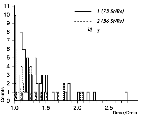
Figure 1: Distribution of ratios of maximal to minimal visual diameters of SNRs from 1 - radio observations (Whiteoak & Green [1996]) and from 2 - an X-ray catalogue (Seward [1990]). The young SNRs, which are expecting to be in the free expansion stage, are separated - 3 (Lozinskaya [1992], Seward [1990], Greiner et al. [1994], Aslanjan [1996], Stankevich [1996]).

We use this method here, but we limit ourselves to the case of equilibrium emissivity. Non-equilibrium effects will be considered in a further paper.

2 Hydrodynamical modelling

As proposed by Hnatyk & Petruk ([1996]) the hydrodynamical description includes two steps: the calculation of shock front dynamics (shape of SNR) and the calculation of the state of the plasma inside the SNR.

2.1 Calculation of shock front motion

Klimishin & Hnatyk ([1981]), Hnatyk ([1987]) have shown that the motion of a strong one-dimensional adiabatic shock wave in a medium with an arbitrary distribution of density is described with high accuracy by the approximate formula:

$${dR\over dt}=D(R)={\rm const}\cdot(\rho^{\rm o}(R)\cdot R^{N+1})^{-k}$$ (1)

where

$$k=\left\{\matrix{1/2,&m(R)\leq N+1&\cr 1/5,&m(R)>N+1&\cr}\right.\ ,$$ (2)

$R$ is the distance from the explosion, $\rho^{o}(R)$ is the initial density distribution of the surrounding medium; $m(R)=-d\ln(\rho^{o}(R))/d\ln R$; $N=0,1,2$ for a plane, cylindrical and spherical shock, respectively.

Formulae (1)-(2) generalize two basic features of shock motion in non-uniform media:

- a deceleration in a medium with increasing $(m(R)<0)$, constant $(m(R)=0)$ or slowly decreasing density $(0<m(R)\leq N+1)$; then the parameter $k$ is close to $k=1/2$;

- an acceleration if the density is decreasing fastly enough as $m(R)>N+1$; then the parameter $k$ is close to $k=1/5$.

Since in all realistic cases $m(0)=0$, i.e. the initial stage of the motion of the shock from a point explosion is always described by the self-similar Sedov solution for a uniform medium, for the deceleration stage of shock motion from eq. (1)-(2) we have:

$$\begin{array}[]{l}D(R)\approx D_{\rm D}(R)=\\ \qquad\quad={\displaystyle{2\over 3+N}\cdot\biggl{(}{E_{o}\over\alpha_{\rm A}(N,\gamma)\cdot\rho^{\rm o}(R)}\biggr{)}^{1/2}\cdot R^{-(N+1)/2}},\end{array}$$ (3)

where $\alpha_{\rm A}(N,\gamma)$ is the self-similar constant for a uniform medium ($\alpha_{\rm A}(0,\ 5/3)=0.6029$, $\alpha_{\rm A}(2,\ 5/3)=0.4936$), $E_{o}$ is the energy of explosion.

If the density distribution is such that a region of acceleration with $m(R)>N+1$ exists and begins at some distance $R_{1}$ where $m(R_{1})=N+1$, then an approximate formula for shock velocity is:

$$D_{\rm A}(R,R_{1})\approx D_{\rm D}(R_{1})\cdot\biggl{(}{\rho^{\rm o}(R_{1})\cdot R_{1}^{N+1}\over\rho^{\rm o}(R)\cdot R^{N+1}}\biggr{)}^{1/5}$$ (4)

Here, $D_{\rm D}(R_{1})$ is determined from (3).

If the density distribution is such that there is a transition from a region of acceleration with $m(R)>N+1$ into a region of deceleration where $m(R)\leq N+1$, then another feature appears. At the beginning, the shock deceleration will be analogous to the motion of an external (forward) shock as described by Nadyezhyn ([1985]) and Chevalier ([1982]). The external shock decelerates with $k\approx 1/5$ and, when its velocity equals velocity $D_{\rm D}(R)$ from (3) the further deceleration is described by $k\approx 1/2$.

Therefore, a general formula for the shock velocity which takes into account the three cases is (Hnatyk [1987]):

$$\begin{array}[]{l}D(R)=\\ \\ \left\{\matrix{D_{\rm D}(R),&0\leq R\leq R_{1}&\cr min[D_{\rm A}(R;R_{2n-1});D_{\rm D}(R)],&R_{2n-1}<R<R_{2n+1}&\cr}\right.\!\!\!\!\!\!\!\!\!\!\!\!\end{array}$$ (5)

where $n=1,2,3...$; $R_{n}$ are zeros of the function $m(R)-(N+1)$ (the points of changing of regimes of shock motion) in increasing order of $R$ in the interval $(0,\infty)$.

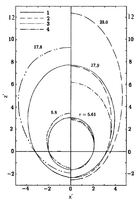
Figure 2: Profiles of a shock front in a non-uniform exponential medium Eq. (11) as a function of dimentionless time $\tau$ (see text). The coordinates are non-dimensional as defined in the text. Line 1 is the result of the numerical 2D calculation; line 2 is the approximate law (5); line 3 is the result of numerical calculation in the sector approximation; line 4 is the result of the thin layer approximation.

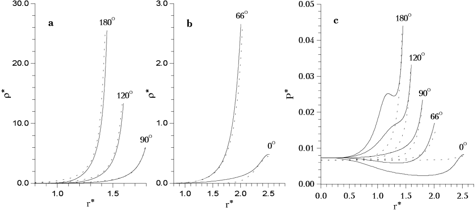
Figure 3: Distributions of density (a, b) and pressure (c) inside an SNR expanding in a flat exponential medium Eq. (11) for different directions from the place of explosion at the dimensionless time $\tau=4.268.$ The solid lines correspond to the present method, the dashed lines are the result of the direct 2D numerical calculations of Kestenboim et al. ([1974]). Here $\gamma=1.4.$

It must be emphasized that the majority of models interesting for astrophysics are described more simply by formulae (3)-(4).

The equation of the trajectory of the shock motion is

$$t=\int\limits_{0}^{R}{dR\over D(R)}.$$ (6)

When the density distribution departs from spherical symmetry, the calculation should be carried out by sectors. The 3D region is divided into the necessary quantity of sectors and Eq. (6) is integrated for each of them. Such an approach allows also to consider an anisotropic energy release $E(\Omega)$ replacing $E_{\rm o}$ by $2\pi NE(\Omega)$ for $N=1,2$.

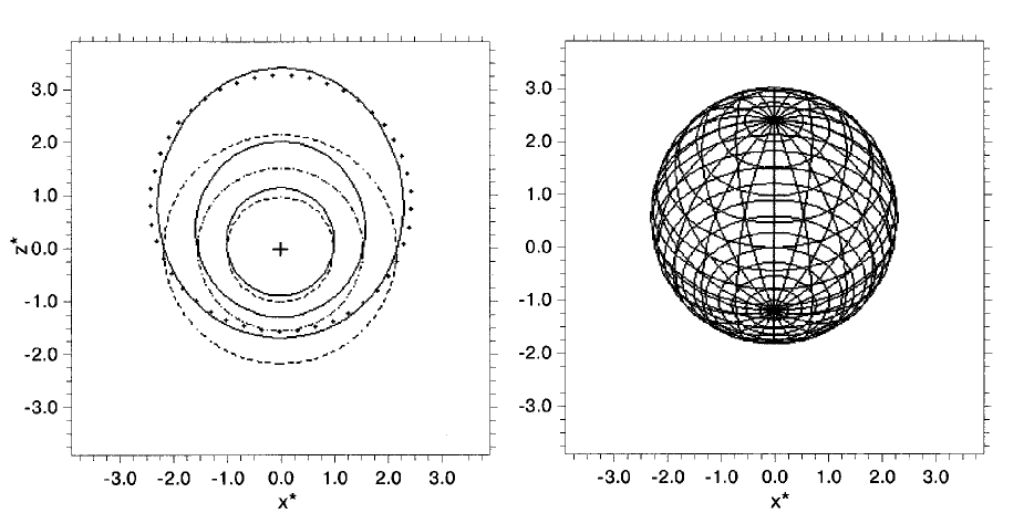
Figure 4: a) Profiles of shock front expanding in a exponential medium Eq. (11) (solid lines) and in a uniform medium (dashed lines) for dimensionless times $\tau=1,\ 3,\ 7$. The dotted line is the profile fitting by a sphere for $\tau=7$. b) The 3D shape of the same SNR for $\tau=7$. The angle between the symmetry axis of the SNR and the plane of sky is $45^{\rm o}$.

2.2 Calculation of the plasma characteristics inside SNR

The second step concerns the determination of gas parameters inside the SNR. It uses on the shock motion law by sector discribed in the previous step. We will use the Lagrangian coordinates $(a,t)$ ($a$ is the initial coordinate of the gas element at $t=0$) and take as the unknown function the position (Eulerian coordinates) of the gas element $r(a,t)$ ($0\leq r(a,t)\leq R$) at time $t$. The function $r(a,t)$ is expanded into series about the shock front and about the center of explosion. Then these two decompositions are combined. The coefficients of decomposition near the shock front is determined by the motion law in each sector and near the center of explosion assuming a zero pressure gradient (see Appendix A.3). It is important that the value of pressure in the central region be taken equal in all sectors contrary to previous propositions (Laumbach & Probstein [1969], Hnatyk [1987], Hnatyk [1988]). The value of pressure around the point of explosion is determined from the condition that the ratio $\eta$ of pressure in the center of explosion $P(0,t)$ to the average value of energy density inside SNR $E_{\rm o}/V_{\rm tot}(t)$ does not change with time and is equal to the self-similar value for a uniform medium:

$$\eta\equiv P(0,t)V_{\rm tot}(t)/E_{\rm o}~{}=~{}\eta_{\rm A}.$$ (7)

In this way, we approximatively take into account a redistribution of energy between the sectors in the cases of an anisotropic explosion and/or a non-uniform medium.

The calculation of $r(a,t)$ is presented in Appendixes A.1-A.3.

The other parameters (pressure $P(a,t)$, density $\rho(a,t)$, velocity $u(a,t)$) are exactly derived from $r(a,t)$ in case of adiabatic motion of gas behind the shock front (Hnatyk [1987]):
– the density is obtained from the continuity equation

$$\rho(a,t)=\rho^{\rm o}(a)\Bigl{(}{a\over r(a,t)}\Bigr{)}^{N}\left({\partial r(a,t)\over\partial a}\right)^{-1};$$ (8)

– the pressure is derived from the equation of adiabaticity $P=K\rho^{\gamma}$ or

$${P(a,t)\over P(R,t)}=\biggl{(}{\rho^{\rm o}(a)\over\rho^{\rm o}(R)}\biggr{)}^{1-\gamma}\biggl{(}{D(a)\over D(R)}\biggr{)}^{2}\biggl{(}{\rho(a,t)\over\rho(R,t)}\biggr{)}^{\gamma};$$ (9)

– velocity directly from approximation $r=r(a,t)$

$$u(a,t)={\partial r(a,t)\over\partial t}.$$ (10)

2.3 Testing the method

The proposed method exactly describes the shock trajectory in self-similar (Sedov) cases with $m(R)={\rm const}\leq N+1,$ including in particular the uniform ($m=0$) medium. The space distributions of the gas parameters: pressure $P(r,t),$ density $\rho(r,t),$ temperature $T(r,t)$ and velocity $u(r,t)$ inside the SNR are accurate within 3% in the $m=0$ case (Hnatyk & Petruk [1996]).

The result of the calculation for a point explosion in medium with an exponential density distribution

$$\rho^{\rm o}(z)=\rho^{\rm o}(0)\cdot\exp\Bigl{(}-{z\over H}\Bigr{)},\quad z=r\cos\theta,$$ (11)

where $r$ is the distance from the center of explosion, $\theta$ is the angle between the considered direction and the direction opposite to the density gradient, and $H$ is the scale height, are presented in fig. 2-3. The simulations are carried out for dimensionless parameters $\tau=t/t_{\rm m},$ $r^{*}=r/R_{\rm m},$ $\rho^{*}=\rho/\rho_{\rm m},$ $P^{*}=P/P_{\rm m},$ with $t_{\rm m}=\alpha_{\rm A}(2,\gamma)^{1/2}E_{\rm o}^{-1/2}\rho_{\rm o}^{1/2}(0)R_{\rm m}^{5/2},$ $R_{\rm m}=H,$ $\rho_{\rm m}=\rho^{\rm o}(0),$ and $P_{\rm m}=\alpha_{\rm A}(2,\gamma)^{-1}E_{\rm o}R_{\rm m}^{-3}.$ They allow to obtain the solution for any value of the initial parameters $E_{\rm o},$ $\rho^{\rm o}(0),$ and $H.$

Fig. 2 presents the results of a direct 2D numerical calculation together with results of different approximate approaches (Kestenboim et al. [1974]). As we see, for the largest time $\tau=17.9,$ the proposed method is accurate within 7%, i.e., of the same order of accuracy as the numerical method. Even a numerical calculation by sector (1D numerical calculation in each sector) yields a considerably lower accuracy, only about 20%.

Another important quantity useful to check the accuracy the shock acceleration in exponential atmosphere is the breakout time $\tau_{\rm br},$ when shock velocity $D(\theta\!=\!0^{\rm o})\to\infty.$ The combination of the 2D numerical solutions for $\tau\leq 17.9$ with the self-similar solution for $\tau>17.9$ for $\gamma=1.4$ yields $\tau_{\rm br}=29.6$ (Kestenboim et al. [1974]) while approximation (5) gives $\tau_{\rm br}=30.8.$

The accuracy of the density and pressure calculations in the proposed method is illustrated by Fig. 3.

Additional results of testing of the method for more complex density distributions, such as a density discontinuity are presented by Hnatyk ([1987]). All these results reveal that the proposed method has high enough accuracy in all cases in the sector aproximation. It fails however in the case of shock interaction with a small dense cloud.

3 SNR shapes in non-uniform media

We now consider the role of the surrounding ISM on the evolution and the X-ray emission of adiabatic SNR on the examples of media with flat exponential and spherically-symmetrical power-law density distributions.

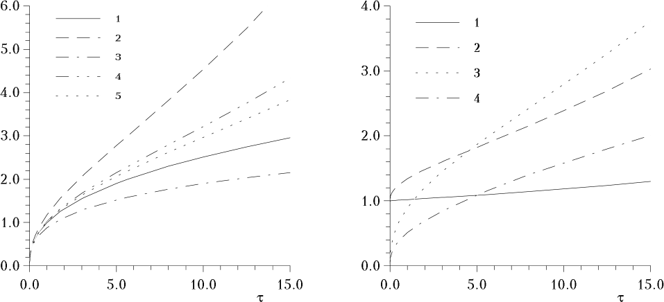
Figure 5: Evolution of the shape and characteristics of a shock wave for a point explosion in a flat exponential medium Eq. (11). a: 1 – radius of shock front $R^{*}_{\pi/2}$ in direction $\theta=90^{\rm o}$ (this equals $R_{\rm s}$ for the case a uniform medium); 2 – $R^{*}_{0}$; 3 – $R^{*}_{\pi}$; 4 – $(R^{*}_{0}+R^{*}_{\pi})/2$; 5 – average visual radius of NSNR in exponential medium. b: 1 – ratio of maximal to minimal diameters of visual shape of shock wave front; 2 – ratio $R_{0}/R_{\pi}$; 3 – $\log(\rho_{\pi}/\rho_{0})$; 4 – $\log(T_{0}/T_{\pi}).$

3.1 Shapes of SNRs in a flat exponential medium

The exponential law distribution is frequently encountered in nature, especially in galactic disks. We consider the evolution of the shape of the shock front from a point explosion in a medium with exponential density distribution Eq. (11). The morphological evolution of such SNR are presented in Fig. 4. We can see from this figure the remarkable insensitivity of the visible form of the SNR to the ISM density gradient.

The apparent center of the non-spherical SNR does not coincide with real progenitor position. This may be important for localizing a possible compact stellar remnant (pulsar or black hole).

The evolution of some shock characteristics is presented in Fig. 5. The main result is that the average visible morphological characteristics of the non-spherical SNRs are usually close to those for Sedov SNRs with the same initial parameters.

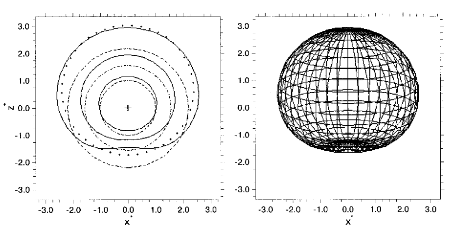
Figure 6: a and b The same as in Fig. 4 for a power law density distribution Eq. (13) for $r_{0}^{*}=1.75$ and $\tau=7.$ The angle between the symmetry axis of NSNR and the plane of the sky in the right figure equals $15^{\rm o}$.

3.2 Shapes of SNRs in a power-law medium

Another widely-used density distribution is the power-law one, created by stellar winds, previous SN explosions etc.:

$$\rho^{\rm o}(\tilde{r})=\rho_{\rm o}(\tilde{r}/R_{\rm m})^{\omega}.$$ (12)

We consider the evolution of the shock from a point explosion in a medium with a spherically-symmetrical power-law density distribution when the explosion point is displaced by a distance $r_{\rm o}$ from the center of symmetry $\tilde{r}=0$ (wind source etc.). Therefore the density distribution as a function of the distance $r$ from the explosion point $r_{\rm o}$ is:

$$\rho^{\rm o}(r,\theta)=\rho^{\rm o}(0){\left({\sqrt{r_{\rm o}^{2}+r^{2}-2rr_{\rm o}\cos\theta}\over r_{\rm o}}\right)}^{w}.$$ (13)

Here $\rho^{\rm o}(0)$ is the initial density in the point of explosion. Hereafter, we take $w=-2$ and $r_{\rm o}=1.75R_{\rm m}$.

The shape evolution of the SNR in this density distribution is shown in Fig. 6. It is worthy to note that visible shapes of such SNRs may be elongated transverse to the density gradient.

As one can see from Fig. 6, b like to the previous case (Fig. 4, b), the projection of the SNR on the plane of the sky can cause a spherization of the visible SNR shape. So, even a visible spherical shape of SNR does not guarantee the uniformity of ISM and isotropy of explosion.

3.3 Discussion

From the above results, it follows that:

1. The non-uniformity of the surrounding medium causes asphericity of SNRs. The visible shapes may be elongated not only along (Fig. 4) but also transverse to (Fig. 6) the density gradient, depending on the type of density distribution.

2. SNR may have an apparent shape close to spherical even in cases of essential anisotropy of the real form and essential gradient of density distribution along the surface.

3. The observed anisotropy of the shape is smaller than the real anisotropy as result of projection. The visible shape remains, generally, close to spherical.

4. The non-uniformity of the surrounding medium results in differences of shock characteristics along the SNR surface. If the initial density $\rho$ varies along the shock surface, the maximal contrasts are expected in the X-ray surface brightness ($\propto\rho^{2}$), they are smaller for the temperature distribution ($\propto\rho$) and minimal in shock and postshock gas velocities ($\propto\rho^{-1/5}$) (Figs. 4–6).

Therefore to determine the real conditions inside and around SNR, it is necessary to use additional information about SNR. We consider further the X-ray observations as an effective tool for SNR diagnostics.

4 Integrated characteristics of the X-ray radiation from non-spherical SNRs

SNRs are powerful sources of X-ray radiation, therefore X-ray observations of SNR give unique information about physical conditions inside the remnants. We calculate here the X-ray luminosities in the energy ranges $\varepsilon=h\nu>0.1\ {\rm keV}$ ($L_{\rm x}^{>0.1}$) and $\varepsilon>4.5\ {\rm keV}$ ($L_{\rm x}^{>4.5}$) as well as the spectral index $\alpha$ at $\varepsilon=5\ {\rm keV}.$

Table 1: Luminosity in ranges $\varepsilon>0.1\ {\rm keV}$ and $\varepsilon>4.5\ {\rm keV}$ (in parenthesis) of SNR expanding in an exponential medium Eq. (11) with $H=10\ {\rm pc}$ (upper lines) in comparison with Sedov SNR (lower lines). The SN explosion energy is $E_{\rm 51}=1$.

$\log(t_{\rm yrs})$	$\tau(n_{\rm H}^{\rm o})^{1/2}$	$\log(n_{\rm H}^{\rm o})$
		-1	-0.5	0	0.5	1
2.5	0.056	-	34.97 (34.66)	35.53 (35.28)	36.12 (35.88)	36.74 (36.42)
		-	34.96 (34.64)	35.52 (35.27)	36.11 (35.87)	36.73 (36.42)
3.0	0.176	34.65 (34.39)	35.26 (34.93)	35.92 (35.42)	36.62 (35.83)	37.35 (36.12)
		34.61 (34.37)	35.23 (34.92)	35.89 (35.41)	36.60 (35.83)	37.34 (36.13)
3.5	0.555	35.25 (34.31)	35.95 (34.61)	36.68 (34.79)	37.43 (34.83)	38.19 (34.80)
		35.10 (34.33)	35.84 (34.63)	36.60 (34.79)	37.38 (34.82)	38.16 (34.78)
3.75	0.987	35.72 (33.94)	36.41 (34.09)	37.13 (34.10)	37.86 (34.06)	38.57 (34.11)
		35.47 (33.98)	36.24 (34.07)	37.02 (34.05)	37.79 (34.03)	38.54 (34.10)
4.0	1.755	36.23 (33.40)	36.89 (33.41)	37.56 (33.37)	38.23 (33.43)	-
		35.88 (33.32)	36.66 (33.28)	37.42 (33.31)	38.15 (33.40)	-
4.25	3.121	36.74 (32.86)	37.30 (32.78)	37.88 (32.79)	-	-
		36.29 (32.53)	37.04 (32.60)	37.74 (32.72)	-	-
4.5	5.555	37.04 (32.54)	37.53 (32.40)	-	-	-
		36.65 (31.90)	37.33 (32.04)	-	-	-

4.1 Plasma X-ray emissivity under ionization equilibrium condition

We assume the cosmic abundance (Allen [1973]). The X-ray continuum energy emissivity per unit energy interval is (in ${\rm erg\ cm^{-3}\ s^{-1}\ keV^{-1}}$)

$$\begin{array}[]{l}P_{\rm c}(T,\varepsilon)=\\ \\ {\displaystyle\qquad=1.652\cdot 10^{-23}n_{\rm e}^{2}G_{\rm c}(T,\varepsilon)T_{6}^{-1/2}exp\left({-11.59\varepsilon\over T_{6}}\right),}\end{array}$$ (14)

where $\varepsilon>0.1$ is the photon energy in keV, $T_{6}$ is the plasma temperature in $10^{6}\ {\rm K}$, $n_{\rm e}$ is the electron number density. The approximation for total Gaunt factor $G_{\rm c}$ as the sum of Gaunt factors for free-free $G_{\rm ff},$ free-bound $G_{\rm fb}$ and two-photon $G_{\rm 2\gamma}$ processes was taken from Mewe et al. ([1986]):

$$G_{\rm c}(T,\varepsilon)=27.83(T_{6}+0.65)^{-1.33}+0.35{\varepsilon}^{-0.34}T_{6}^{0.422}.$$ (15)

This approximation represents the continuum losses to an accuracy of $10-20\%$ for $T\geq 3\cdot 10^{6}\ {\rm K}$ and of $30-50\%$ for $T=(0.2-3)\cdot 10^{6}\ {\rm K}$.

For calculation of continuum and line emission of plasma in the different energy ranges, we have approximated the Raymond & Smith ([1977]) data for plasma emissivity $\Lambda$ (in ${\rm erg\ cm^{-3}\ s^{-1}}$)
for $\varepsilon=0.1-2.4\ {\rm keV}$ as follows:

$$\Lambda^{0.1-2.4}(T)=10^{-21.80}T_{6}^{-0.63}\exp\left({-1.40\over T_{6}}\right),$$ (16)

(accurate to $5-30\%$ for $\log T=5.3-8$);
for $\varepsilon>4.5\ {\rm keV}$ as follows:

$$\Lambda^{>4.5}(T)=10^{-22.42}\exp\left({-39.50\over T_{6}^{0.77}}\right),$$ (17)

(accurate to $1-8\%$ for $\log T=6.7-8$);
for $\varepsilon>0.1\ {\rm keV}$ as follows:

$$\Lambda^{>0.1}(T)=\Lambda^{0.1-2.4}(T)+10^{-24.4}T_{6}^{0.8},$$ (18)

(accurate to $7-35\%$ for $\log T=5.5-8$).

The total flux $F_{\varepsilon}$ at photon energy $\varepsilon$ and luminosity $L_{\rm x}$ of the entire SNR can be calculated by integrating over the remnant volume $V$

$$F_{\varepsilon}=\int\limits_{V}P_{\rm c}(T,\varepsilon)dV,$$ (19)

$$L_{\rm x}=\int\limits_{V}\Lambda(T)n_{\rm e}n_{\rm H}dV.$$ (20)

The spectral index $\alpha$ is

$$\alpha=-{\partial\ln F_{\varepsilon}\over\partial\ln\varepsilon}.$$ (21)

4.2 Evolution of the total X-ray emission from aspherical SNRs

It is well-known that the Sedov ([1959]) solution for SNR characteristics in a uniform medium is determined by three parameters, e.g., the energy of the explosion $E_{\rm o}=10^{51}E_{51}\ {\rm erg},$ the initial number density $n_{\rm H}^{\rm o}$ and time $t$. The shape of the integrated spectrum (in particular the spectral index $\alpha$) depends only on one parameter (the shock temperature $T_{\rm s}$) in case of collision ionization equilibrium (CIE) and on two ($T_{\rm s}$ and $\eta=E_{\rm o}\left(n_{\rm H}^{\rm o}\right)^{2}$) in case of NEI (for fixed abundance) (Hamilton et al. [1983]). In order to estimate the total luminosity of a Sedov SNR in the NEI case, we need a third parameter, i.e. the explosion energy $E_{\rm o}$ (Hamilton et al. [1983]). In the Sedov CIE case the luminosity depends only on two parameters $T_{\rm s}$ and $\zeta=E_{\rm 51}n_{\rm H}^{\rm o}.$

If the SN explodes in a non-uniform medium, we have an additional fourth parameter which characterises the non-uniform density distribution. In our cases, it is the scale height $H$ for exponential density distribution or $r_{\rm o}$ for power-law density distribution.

Table 2: Spectral index $\alpha(5\ keV)$ of NSNR in exponential medium Eq. (11) with $H=10\ pc$ (upper lines) in comparison with Sedov SNR (lower lines). The SN explosion energy is $E_{\rm 51}=1$.

$\log(t_{\rm yrs})$	$\tau(n_{\rm H}^{\rm o})^{1/2}$	$\log(n_{\rm H}^{\rm o})$
		-1	-0.5	0	0.5	1
2.5	0.056	-	0.49	0.58	0.71	0.92
		-	0.49	0.57	0.70	0.91
3.0	0.176	0.75	0.95	1.26	1.74	2.47
		0.70	0.91	1.23	1.72	2.45
3.5	0.555	1.95	2.57	3.46	4.52	5.05
		1.72	2.45	3.49	4.67	5.06
3.75	0.987	3.06	3.81	4.70	4.89	4.24
		2.93	4.10	5.04	4.78	4.22
4.0	1.755	3.80	4.56	4.73	4.07	-
		4.67	5.06	4.45	4.05	-
4.25	3.121	4.02	4.55	4.01	-	-
		4.78	4.21	3.94	-	-
4.5	5.555	3.60	3.82	-	-	-
		4.05	3.85	-	-	-

Table 3: The same as in Table 1 for $E_{\rm 51}=0.1$ and range $\varepsilon>0.1\ {\rm keV}$.

$\log(t_{\rm yrs})$	$\tau(n_{\rm H}^{\rm o})^{1/2}$	$\log(n_{\rm H}^{\rm o})$
		-1	-0.5	0	0.5	1
2.5	0.018	-	34.12	34.74	35.40	36.10
		-	34.11	34.73	35.39	36.10
3.0	0.056	33.92	34.62	35.35	36.11	36.89
		33.89	34.60	35.34	36.11	36.88
3.5	0.176	34.68	35.43	36.19	36.94	37.66
		34.60	35.38	36.16	36.92	37.65
4.0	0.555	35.56	36.23	36.86	37.43	37.90
		35.42	36.15	36.83	37.43	37.90

Table 4: The same as in Table 2 for $E_{\rm 51}=0.1$.

$\log(t_{\rm yrs})$	$\tau(n_{\rm H}^{\rm o})^{1/2}$	$\log(n_{\rm H}^{\rm o})$
		-1	-0.5	0	0.5	1
2.5	0.018	-	0.71	0.92	1.23	1.72
		-	0.70	0.91	1.23	1.72
3.0	0.056	1.26	1.74	2.47	3.49	4.66
		1.23	1.72	2.45	3.49	4.67
3.5	0.176	3.46	4.52	5.05	4.48	4.05
		3.49	4.67	5.06	4.45	4.05
4.0	0.555	4.73	4.07	3.87	3.76	3.68
		4.45	4.05	3.85	3.74	3.66

Table 5: The ratios of SNR characteristics (the volume $V$, swept-up mass $M$ and characteristic temperatures $T_{\rm ch}$) in non-uniform medium (with exponential (E) Eq. (11) and power law (PL) Eq. (13) density distribution) to uniform ones.

$\tau$	$V/V_{{\rm s}}$			$M/M_{{\rm s}}$			$T_{\rm ch}/T_{s}$
	E	PL		E	PL		E	PL
0.1	1.00	1.02		1.00	1.00		1.00	1.00
0.5	1.03	1.06		1.00	0.99		1.00	1.01
1.0	1.05	1.10		1.01	0.98		0.99	1.02
3.0	1.14	1.24		1.01	0.95		0.99	1.06
5.0	1.23	1.37		1.02	0.92		0.98	1.09
10.0	1.51	1.64		1.04	0.86		0.96	1.16
20.0	2.53	2.13		1.07	0.75		0.94	1.33

It is naturally to expect, that in cases of NSNR considered, the total X-ray luminosity $L_{\rm x}$ as well as spectral index $\alpha$ will strongly depend on non-uniformity characteristics, such as scale height $H$ etc. Therefore, we calculate here extensive grid of models for evolution of X-ray radiation from NSNRs which evolve in non-uniform ISM and compare it with the Sedov case. Our grid covers the range of paramers which correspond to the adiabatic stage of SNR evolution, i.e. for SNR radii between $R_{\rm i}=\left(3M_{\rm ej}/4\pi\rho^{\rm o}(0)\right)^{1/3}\simeq 2.5(n_{\rm H}^{\rm o})^{-1/3}\ {\rm pc}$ when the swept up mass of ISM becomes equal to the mass of ejecta $M_{\rm ej}\simeq 1M_{\sun},$ and $R_{\rm f}$ when the effective temperature $T_{\rm ef}$ corresponds to the maximum value of plasma emissivity function $T_{\rm ef}\simeq 1.3T_{\rm s}=5.2\cdot 10^{5}\ {\rm K}$ (Lozinskaya [1992]). In a non-uniform medium, the value of $R_{\rm f}$ depends on the concrete density distribution in a selected direction (sector). So, if the density distribution in a sector is exponential $n_{\rm H}^{\rm o}(r)=n_{\rm H}^{\rm o}(0)\cdot\exp(\pm r/H),$ we may estimate $R_{\rm f}$ from the relation $R_{\rm f}\cdot\exp(\pm R_{\rm f}/3H)=25(E_{\rm 51}/n_{\rm H}^{\rm o}(0))^{1/3}\ {\rm pc}.$ For a uniform medium $H=\infty,$ we obtain $R_{\rm max}\simeq 25E_{\rm 51}^{0.3}(n_{\rm H}^{\rm o}(0))^{-0.3}\ {\rm pc},$ which is close to results of other authors (Lozinskaya [1992]). In our calculation, the maximal time was estimated from adiabaticity violation in the $\theta=\pi/2$ sector. For parameters of ISM considered here, maximal radii of SNRs do not exceed a few scale heights. Therefore, obtained results are not affected by shock acceleration, which is important only at considerably greater distances.

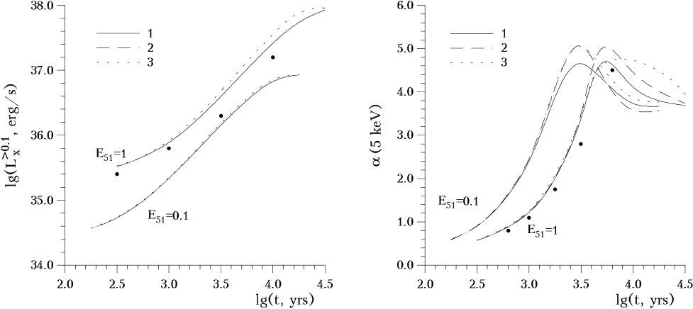
Figure 7: Evolution of luminosity $L_{\rm x}$ in range $>0.1\ {\rm keV}$ and of spectral index $\alpha(5\ {\rm keV})$ of SNRs in a uniform medium (line 1), in an exponential medium Eq. (11) with $H=80\ {\rm pc}$ (line 2) and $H=10\ {\rm pc}$ (line 3). In all cases $n_{\rm H}^{\rm o}(0)=1\ {\rm cm^{-3}}$. Results of numerical calculations of Hamilton et al. ([1983]) for a uniform medium and $E_{51}=1$ with Meyer abundance are also shown by dots. Hereafter $\gamma=5/3$.

We show in Fig. 7 the evolution of X-ray luminosity for range $\varepsilon>0.1\ {\rm keV}$ and spectral index $\alpha$ at $5\ {\rm keV}$ for SNR in an exponential medium. It is easy to see that both X-ray characteristics of NSNR evolve analogously to the Sedov case and similarity increases with decreasing surrounding medium density gradient (with increasing $H$) and decreasing explosion energy. The results presented in Fig. 7 of calculations of the Sedov case for $E_{\rm 51}=1$ (Hamilton et al. [1983]) reveal some differences between X-ray luminosities at low temperatures. They may be caused, in part, by atomic data and chemical composition differences (our model uses the Allen abundance, whereas in the paper of Hamilton et al. ([1983]) have been used the Meyer abundance). Our results for Sedov case coinside with of Leahy & Aschenbach ([1996]) and Kassim et al. ([1993]) results for model with Allen abundance within 25%.

Table 6: Evolution of SNR luminosity $L_{\rm x}$ and spectral index $\alpha(5\ {\rm keV})$ in uniform (S) and exponential (E) Eq. (11) media.

				$\log\zeta=\log(n_{\rm H}^{\rm o}\cdot E_{\rm 51})$
$\log(T_{\rm ch})$	model	H	$E_{\rm 51}$		-1				0				1
				$\tau$	$L_{\rm x}^{>0.1}$	$\alpha_{5}$		$\tau$	$L_{\rm x}^{>0.1}$	$\alpha_{5}$		$\tau$	$L_{\rm x}^{>0.1}$	$\alpha_{5}$
8.0	S				34.68	0.81			35.68	0.81			36.68	0.81
	E	80	1	0.004	34.68	0.82		0.001	35.68	0.82		8e-5	36.68	0.81
	E	10	0.1	0.015	34.68	0.82		0.002	35.68	0.82		3e-4	36.68	0.82
	E	10	1	0.696	34.73	0.88		0.102	35.69	0.83		0.015	36.68	0.82
7.2	S				35.49	3.02			36.49	3.02			37.49	3.02
	E	80	1	0.018	35.50	3.03		0.003	36.50	3.03		4e-4	37.49	3.02
	E	10	0.1	0.070	35.51	3.03		0.010	36.50	3.03		0.001	37.50	3.03
	E	10	1	3.232	35.75	3.13		0.474	36.56	3.05		0.070	37.51	3.03
6.4	S				36.56	4.18			37.56	4.18			38.56	4.18
	E	80	1	0.083	36.57	4.19		0.012	37.56	4.18		0.002	38.56	4.18
	E	10	0.1	0.323	36.59	4.20		0.047	37.57	4.18		0.007	38.56	4.18
	E	10	1	15.00	36.98	3.73		2.202	37.70	4.38		0.323	38.59	4.20

We have calculated a grid of NSNR models (Tables 1-4) which confirms that this analogy in evolution is an intrinsic property of NSNR X-ray radiation. In fact, it may be seen from Tables 1-4 that for a wide range of number density at the point of explosion $n_{\rm H}^{\rm o}(0)=0.1-10\ {\rm cm^{-3}},$ the X-ray luminosity of adiabatic NSNR evolving in a medium with strong enough density gradient ($H=10\ {\rm pc}$) in different energy ranges are not far from the X-ray luminosity of SNR in a uniform density medium with the same initial model parameters. The differences increase with age of the SNR and with decreasing $n_{\rm H}^{\rm o}(0)$. But even for old NSNR (e.g., $t=3\cdot 10^{4}\ {\rm years}$) in a low density medium ($n_{\rm H}^{\rm o}(0)=0.1\ {\rm cm^{-3}}$), the maximal difference is about $60\%$ (for $\tau=17.5$). The differences in spectral index of adiabatic NSNR do not exceed $10\%$. Table 1 shows that luminosity in range $\varepsilon>4.5\ {\rm keV}$ is close to the Sedov case also. These last two facts reveal the similarity of total spectra of Sedov SNR and non-spherical ones.

We suppose that the behevior of integral X-ray characteristics of NSNR in other cases of smooth continuous density distribution of surrounding medium will be similar considered above, since X-ray emission mainly depends on the emission measure $EM\simeq n_{\rm e}^{2}V\simeq M^{2}V^{-1},$ but both masses of swepted up gas $M$ and volume of NSNR $V$ remain close to those of Sedov SNR (Table 5). Moreover, the last fact allow us to introduce a characteristic shock temperature for NSNR $T_{\rm ch}$, comparable to $T_{\rm s}$ in the Sedov case:

$$T_{\rm ch}^{*}={32\pi\over 75}{{\gamma-1}\over{(\gamma+1)^{2}}}(M^{*})^{-1},$$ (22)

where $T^{*}=T/T_{\rm m},$ $M^{*}=M/M_{\rm m}$ with $T_{\rm m}=\alpha_{\rm A}(2,\gamma)^{-1}A_{\rm gas}^{-1}E_{\rm o}\rho_{\rm o}^{-1}(0)R_{\rm m}^{-3}$ and $M_{\rm m}=\rho_{\rm o}(0)R_{\rm m}^{3}.$ The temperature $T_{ef}$ determined from the observed spectrum will be connected with $T_{\rm ch}$ as in the Sedov case $T_{ef}\approx 1.3T_{\rm ch}$ (Itoh [1977]). This characteristic temperature may be used to estimate the parameters of the whole remnant, such as mass, volume, etc.

The results of calculations show that integral X-ray characteristics weakly depend on the surrounding medium density gradient (e.g., $H$). Therefore, as in the Sedov case, a spectral index of equilibrium emission from NSNR depends approximately only on one parameter $T_{\rm ch}$ and luminosity depends approximately only on two parameters: $T_{\rm ch}$ and $\zeta=E_{\rm 51}n_{\rm H}^{\rm o}(0)$. As confirmation of this, we show that maximal deviation from this rule for NSNR in exponential density distribution reaches few percent for spectral index and a few tens of percent for luminosity (Table 6).

4.3 Discussion

From Fig. 7 and Tables 1-6 follows a remarkable fact of proximity of total fluxes and spectrum shapes of SNRs in uniform and non-uniform media even in case of considerable anisotropy of adiabatic NSNR. The reason of this phenomenon is mutual compensation of emission deficit from low density regions of NSNR and enhanced emission from high density regions. This explains the strange circumstance that integral X-ray characteristics of the majority of SNRs with evident asymetry in shape and/or surface brightness distribution are described with sufficient accuracy by the Sedov model of SN explosion in a uniform medium. For more correct modelling of physical conditions inside and outside the SNR, it is necessary to analyze the characteristics of X-ray emission distributed over the SNR surface.

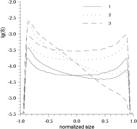
Figure 8: Distribution of $\varepsilon\!>\!0.1\ {\rm keV}$ surface brightness $S^{>0.1}$ along the NSNR symmetry axis in uniform and exponential Eq. (11) media for time moments $t=1000$ yrs (line 1), 5000 yrs (line 2), 40000 yrs (line 3). The model parameters are $E_{\rm 51}=1,$ $n_{\rm H}^{\rm o}(0)=1\ {\rm cm^{-3}},$ $H=10\ {\rm pc}.$

7.5 cm

Figure 9: Distribution of surface brightness $S^{>0.1}$ of the Sedov SNR in uniform medium in the range $\varepsilon>0.1\ {\rm keV}$. The model parameters are $E_{\rm 51}=1,\ n_{\rm H}^{\rm o}(0)=0.2\ {\rm cm^{-3}},\ t=1000\ {\rm yrs}$. The SNR characteristics are $\log(L_{\rm x}^{>0.1},\ {\rm erg/s})=34.98,$ $M=9.4\ {\rm M_{\odot}},$ $T_{\rm s}=9.9\cdot 10^{7}\ {\rm K}$. The lines of constant brightness are indicated by values of logarithm of flux $\log(S)$. The center of explosion hereafter is at the origin of the coordinates.

20.6 cm

Figure 10: The same as in Fig. 9 for exponential medium Eq. (11) with $H=10\ {\rm pc}$. The NSNR parameters at this time are $\log(L_{\rm x}^{>0.1},\ {\rm erg/s})=35.02,\ M=9.4\ {\rm M_{\odot}},\ T_{\rm ch}=9.9\cdot 10^{7}\ {\rm K}$. The NSNR inclination angle to the plane of the sky equals $0^{\rm o}$ (upper case), $45^{\rm o}$ (center case) and $90^{\rm o}$ (lower case).

20.60 cm

Figure 11: The same as in Fig. 10 for time $t=3300\ {\rm yrs}$ ($\log(L_{\rm x}^{>0.1})=35.70,\ M=40.0\ {\rm M_{\odot}},\ T_{\rm ch}=2.3\cdot 10^{7}\ {\rm K}$) and $t=25500\ {\rm yrs}$ ($\log(L_{\rm x}^{>0.1})=37.28,\ M=476\ {\rm M_{\odot}},\ T_{\rm s}=2.0\cdot 10^{6}\ {\rm K}$).

5 Surface - distributed characteristics of NSNR X-ray emission

5.1 Surface brightness in range $\varepsilon>0.1\ {\rm keV}$

We analyse here the surface brightness distribution $S(x,z)$ (in ${\rm erg\ s^{-1}\ cm^{-2}\ ster^{-1}}$)

$$S(x,z)={1\over 4\pi}\int\limits_{y_{1}}^{y_{2}}\Lambda(T)n_{\rm e}n_{\rm H}dy$$ (23)

and surface distribution of spectral index

$$\alpha(x,z)=-{\partial\ln\over\partial\ln\varepsilon}\int\limits_{y_{1}}^{y_{2}}P_{\rm c}(T,\varepsilon)dy,$$ (24)

where the integrals are taken along the line of sight inside the remnant.

5.1.1 NSNRs in a medium with flat exponential density distribution

Figs. 8–11 demonstrate an evolution of surface brightness of NSNR in media with exponential density distribution (11). At the beginning of SNR evolution, the surface brightness map is very like the Sedov one (Fig. 9), but with age the differences become more considerable when the majority of emission arises from more dense regions. The brightness contrast $S_{\rm max}/S_{\rm min}$ may increase with time up to $\sim 10^{5}$ ($S_{\rm max}$ and $S_{\rm min}$ are the values of both the biggest and the smallest maxima in distribution of surface brightness).

In order to interpret an observation, it is necessary to take into account that projection effects also essentially affect the visible morphology of NSNR. Three cases of projection are shown. We can see that projection decreases real anisotropy and contrasts. For example, under condition of full disclosure of NSNR at the age $t=3300\ {\rm years}$ (Fig. 11) $S_{\rm max}/S_{\rm min}=425$ but for inclination angle $45^{\rm o}$ this ratio is $S_{\rm max}/S_{\rm min}=75$.

It is interesting also to compare Fig. 9 and a bottom case of Fig. 10 (when a visible shape of NSNR is spherical as result of projection). One can see that even spherically symmetric Sedov-like observational distribution of surface brightness does not guarantee an isotropic distribution of parameters inside SNR i.e., uniformity of ISM density and isotropy of explosion.

20.60 cm

Figure 12: Distribution of surface brightness $S^{>0.1}$ of NSNR in medium with power-law density distribution Eq. (13) in range $\varepsilon>0.1\ {\rm keV}$. Model parameters are: $E_{\rm 51}=1,$ $n_{\rm H}^{\rm o}(0)=0.2\ {\rm cm^{-3}},$ $t=17800\ {\rm yrs},$ $r_{\rm o}=-17.5\ {\rm pc}$. The NSNR inclination angle to the plane of the sky equals $0^{\rm o}$ (upper case), $45^{\rm o}$ (center case), and $90^{\rm o}$ (lower case).

7.5 cm

Figure 13: The same as in Fig. 10 for range $\varepsilon>4.5\ {\rm keV}$ and time $t=3300\ {\rm yrs}$ ($\log(L_{\rm x}^{>4.5})=34.48$) and $t=25500\ {\rm yrs}$ ($\log(L_{\rm x}^{>4.5})=32.58$).

5.1.2 NSNRs in a medium with power-law density distribution

Fig. 12 shows three projections of NSNR in power-law density distribution (13) with $E_{\rm 51}=1,$ $n_{\rm H}^{\rm o}(0)=0.2\ {\rm cm^{-3}},$ $t=1000\ {\rm yrs}$. Corresponding NSNR characteristics are $\log(L_{\rm x}^{>0.1})=37.03,$ $M=268\ {\rm M_{\odot}},$ $T_{\rm ch}=3.5\cdot 10^{6}\ {\rm K}$. It may be compared with values calculated for NSNRs which evolve in media with different density distribution, to show that different ISM density distributions give similar integral (surface-integrated) X-ray characteristics. For the same model parameters in case of SNR in uniform density, we obtain $\log(L_{\rm x}^{>0.1})=36.75,$ $M=299\ {\rm M_{\odot}},$ $T_{\rm s}=3.1\cdot 10^{6}\ {\rm K}$ and for exponential NSNR: $\log(L_{\rm x}^{>0.1})=37.08,$ $M=308\ {\rm M_{\odot}},$ $T_{\rm ch}=3.0\cdot 10^{6}\ {\rm K}.$

As result of projection, the maximum of surface brightness does not lie close to the edges of NSNR as in shell-like SNRs, but creates a compact region inside the visible projection. Therefore, the projection effect in case of the NSNR elongated predominantly along the line of sight is one possible sources of apparent filled-centre SNRs, especially when the search for a pulsar has no result.

5.2 Surface brightness in range $\varepsilon>4.5\ {\rm keV}$

Different photon energy ranges reveal different sensitivity to the non-uniformity of ISM. Fig. 13 shows the results of calculation of surface brightness of NSNR in an exponential density distribution (11) in range $\varepsilon>4.5\ {\rm keV}$. We may see that surface brightness contrast in this range is essentially smaller then in the wider range $\varepsilon>0.1\ {\rm keV},$ where line emission dominates. So, for $t=3300\ {\rm years}$ (Fig. 11) the maximal surface brightness contrast is $S_{\rm max}/S_{\rm min}=425$ for $\varepsilon>0.1\ {\rm keV}$ and is only $S_{\rm max}/S_{\rm min}=7$ for $\varepsilon>4.5\ {\rm keV}$. A contrast of surface brightness in range $>0.1\ {\rm keV}$ is mainly caused by the contrast of the surrounding medium density distribution ($S\propto\rho^{2}$), but in range $>4.5\ {\rm keV},$ it weakly depends on density contrast ($S\propto\rho^{1/2}$) (Hnatyk & Petruk [1996]).

5.3 Surface distribution of spectral index

Plasma in different regions of NSNR is under different conditions which influence emission. Therefore, spectra from different NSNR regions must be different. The spectral index distribution for NSNR in an exponential medium is shown in Fig. 14. The contrast of values of spectral index increases with time but even for old adiabatic NSNR does not exceed a few times. Meantimes, the projection effects decrease both the index contrast and anisotropy of its distribution.

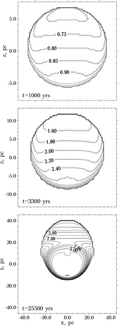
Figure 14: Surface distribution of spectral index $\alpha$ at 5 keV for NSNR in exponential medium Eq. (11) with $H=10\ {\rm pc},$ $E_{\rm 51}=1,$ $n_{\rm H}^{\rm o}(0)=0.2\ {\rm cm^{-3}}$ for time $t=1000\ {\rm yrs}$ (spectral index from total SNR $\alpha^{tot}(5\ {\rm keV})=0.86$), $t=3300\ {\rm yrs}$ ($\alpha^{tot}(5\ {\rm keV})=2.39$) and $t=25500\ {\rm yrs}$ ($\alpha^{tot}(5\ {\rm keV})=3.95$).

5.4 Discussion

We will summarize the results presented in this section.

1. The distribution of surface brightness of NSNR differs essentially from a spherical one.

2. The contrast of surface brightness increases with the age of the SNR and may reach a few ten of thousands.

3. Projection effects hide real contrasts of surface characteristics of NSNR’s emission. Observational morphology of NSNR depends essentially on its orientation to the line of sight.

4. A harder X-ray range (e.g., $\varepsilon>4.5\ {\rm keV}$) is less sensitive to the influence of surrounding medium non-uniformity than a range which includes soft emission. This fact may be used for testing ISM non-uniformity.

5. The surface distribution of spectral index $\alpha$ may also be an effective test for NSNR diagnostics.

6 Conclusions

Large-scale non-uniformity of ISM density distribution in the SN neighborhood essentially affect the evolution of SNR. The shape of SNR becomes essentially non-spherical and distributions of parameters inside the remnant, as viewed from the center of explosion, are strongly anisotropic. We have proposed a new approximate analytical method for full hydrodynamical description of 3D point-like explosions in non-uniform media with arbitrary density distribution i.e., for cases, when well-known self-similar Sedov solutions are inacceptable. On the basis of it, we carry out the simulation of evolution of 2D non-spherical SNRs with special attention to their X-ray radiation. Since our aim in this paper was to investigate the role of density gradients in NSNR evolution, we restricted ourself with the ionization equilibrium case in the calculation of X-ray radiation. The role of electron conductivity, nonequilibrium and nonequipartition effects will be investigated elsewhere.

At first, we have investigated the shape of NSNR and brought out a remarkable fact of sphericity of visible shape of NSNR, even if the real deviation from sphericity is large. When $R_{\rm max}/R_{\rm min}<2,$ the observed shape will differ from spherical by less than $5\%$. Visual shape becomes noticeably non-spherical (more than 5% of visual assymetry) only for surface density contrast of order 100. Projection effects on the sky plane decrease the real shape anisotropy.

Therefore, we have calculated the equilibrium X-ray emission characteristics of NSNR. Again, the total (surface-integrated) parameters of X-ray radiation (luminosity, spectral index) are close to those in Sedov case with the same initial data. This is why many SNRs with apparently 2D anisotropic distribution of X-ray surface brightness are well described by the Sedov model.

Contrary to previous cases of weak dependence of shape and integral X-ray emission characteristics on density gradient, the distribution of X-ray emission characteristics along the surface of NSNR are very sensitive to an initial density distribution arround SN. Moreover, contrast of X-ray surface brightness $S$ caused by density inhomogenity is most prominent, i.e., higher than density or temperature contrasts along the NSNR surface. For case of NSNR in Fig. 11 ($t=3300\ {\rm yrs}$), surface brightness contrast is $S_{\rm max}^{>0.1}/S_{\rm min}^{>0.1}=425,$ but contrast of shock density equals 10 and of shock temperature equals 4 only.

Therefore, the surface brightness maps give the most promising information concerning the physical conditions inside and outside NSNR. It is important to note that typical contrasts of surface brightness caused by density inhomogenity (up to $\sim 10^{5}$) are considerably higher than those caused by nonequilibrium effects. Therefore, the role of density gradient is dominant in interpretation of NSNR observations.

Appendix A Appendix

A.1 Lagrangian form of hydrodynamical equations and shock conditions

We use the set of hydrodynamical equations for the case of one- dimensional adiabatic motion of nonviscous perfect gas in Lagrangian form (Klimishin [1984])

$$\rho_{t}+{\rho^{2}\over\rho^{o}}\Bigl{(}{r\over a}\Bigr{)}^{N}u_{a}+{{Nu\rho}\over r}=0,$$ (25)

$$u_{t}+{1\over\rho^{o}}\Bigl{(}{r\over a}\Bigr{)}^{N}P_{a}=0,$$ (26)

$$P_{t}-c^{2}\rho_{t}=0,$$ (27)

$$r_{t}-u=0.$$ (28)

Here gas pressure $P(a,t)$, its density $\rho(a,t)$, velocity $u(a,t)$ and Eulerian co-ordinate $r(a,t)$ are functions of Lagrangian co-ordinate, i.e., initial gas particle position $a$ and time $t$, $c=\sqrt{\gamma P/\rho}$ is the adiabatic sound velocity, $\gamma$ is the adiabatic index. Subscripts indicate partial derivatives with respect to corresponding variables, $\rho^{o}=\rho^{o}(a)$ is the initial density distribution.

The continuity equation (A-4) may be written in the following form

$$\rho^{o}\cdot a^{N}\cdot da=\rho\cdot r^{N}\cdot dr$$ (29)

or

$$r_{a}={\rho^{o}\over\rho}\Bigl{(}{a\over r}\Bigr{)}^{N}$$ (30)

At front of a strong shock with trajectory $R=R(t),$ the following conditions are satisfied

$$u^{\rm s}=\omega\dot{R}$$ (31)

$$\rho^{\rm s}=(\rho^{o})^{\rm s}/(1-\omega)$$ (32)

$$P^{\rm s}=\omega(\rho^{o})^{\rm s}\dot{R}^{2}$$ (33)

$$r^{\rm s}=R$$ (34)

where $\dot{R}=dR/dt$ is the shock velocity, superscript ”s” corresponds to values of parameters at the shock front $a=R,\ \omega=2/(\gamma+1)$.

A.2 Derivatives of functions of parameter distribution at the shock front

Equations ( -1) - ( -5) and shock conditions ( -6) - ( -9) allow to find the values of arbitrary order partial derivatives of hydrodynamical functions at the shock front using the law of shock motion $R=R(t)$ (Gaffet [1978]).

To find first derivatives of functions $\rho,\ P$ and $u$ at front, we use equations ( -1) - ( -3), written for $a=R$, and add three equations, resulting from differentiation of boundary conditions ( -6) - ( -8) along the shock trajectory by operator $D/Dt=(\partial/\partial t)+\dot{R}(\partial/\partial a)$. Solving the obtained set of six equations for six unknown partial derivatives at the shock front, we obtain expressions for $u^{\rm s}_{a},\ u^{\rm s}_{t},\ P^{\rm s}_{a},\ P^{\rm s}_{t},\ \rho^{\rm s}_{a},\ \rho^{\rm s}_{t}$ (Hnatyk & Petruk [1996]).

From equation ( -5), we have now

$$\begin{array}[]{l}r^{\rm s}_{a}=1-\omega,\\ \\ r^{\rm s}_{t}=u^{\rm s},\\ \\ Rr^{\rm s}_{aa}=\omega(1-\omega)\bigl{[}3B+N(2-\omega)-m\bigr{]}\end{array}$$ (35)

where $B=R\ddot{R}/\dot{R}^{2},\qquad m\equiv m(R)=-(dln\rho/dlna)^{\rm s}$.

To find second derivatives of hydrodynamical functions at the shock front we differentiate equations ( -1) - ( -3) separately with respect to $a$ and $t,$ at the shock front (a=R), what gives us six equations for nine unknown derivatives. Additional three equations are given by differentiation of shock conditions ( -6) - ( -8) by the operator

$${D^{2}\over Dt^{2}}={\partial^{2}\over\partial t^{2}}+2\dot{R}{\partial^{2}\over\partial a\partial t}+\dot{R}^{2}{\partial^{2}\over\partial a^{2}}+\ddot{R}{\partial\over\partial a}.$$ (36)

Solving the system of nine equations with nine unknowns, we obtain expressions for $u^{\rm s}_{at},\ u^{\rm s}_{aa},\ \rho^{\rm s}_{aa}$ (Hnatyk & Petruk [1996]). From ( -5) we obtain

$$\begin{array}[]{l}R^{2}r^{\rm s}_{aaa}=\omega(1-\omega)\Bigl{[}3(7-5\omega)B^{2}+\\ \qquad\quad+\bigl{[}(-5\omega^{2}+4\omega+8)N+(4\omega-11)m\bigr{]}B+\\ \qquad\quad+\omega(2\omega^{2}-7\omega+6)N^{2}+(\omega^{2}+\omega-4)Nm-\\ \qquad\quad-\omega(2-\omega)N-(\omega-2)m^{2}+(2\omega-1)m+\\ \qquad\quad+(2\omega-1)m^{\prime}+(6\omega-4)Q\Bigr{]}\end{array}$$ (37)

where $Q=R^{2}R^{(3)}/\dot{R}^{3},\ \ \ m^{\prime}=-dm/dlnR=-R\cdot dm/dR$.

The time derivative $(r^{\rm s}_{a})_{t}=0$, and for other ones we have

$${R\over\dot{R}}\cdot(Rr^{\rm s}_{aa})_{t}=\omega(1-\omega)\bigl{[}3(B+Q-2B^{2})+m^{\prime}\bigr{]}$$ (38)

$$\begin{array}[]{l}{\displaystyle{R\over\dot{R}}\cdot(R^{2}r^{\rm s}_{aaa})_{t}=\omega(1-\omega)\Bigl{[}3(7-5\omega)\cdot 2B(B+Q-2B^{2})+}\\ \quad+\bigl{[}(-5\omega^{2}+4\omega+8)N+(4\omega-11)m\bigr{]}\cdot\\ \qquad\qquad\qquad\qquad\cdot(B+Q-2B^{2})-\\ \quad-\bigl{[}(4\omega-11)B+(\omega^{2}+\omega-4)N+6(1-\omega)m\bigr{]}m^{\prime}-\\ \quad-(2\omega-1)\bigl{[}(2m+1)m^{\prime}+m^{\prime\prime}\bigr{]}+\\ \quad+2(3\omega-2)\bigl{[}2Q+L-3BQ\bigr{]}\Bigr{]}\end{array}\!\!\!\!\!\!\!\!\!\!\!\!\!\!\!\!\!\!\!\!\!\!\!\!\!\!\!\!\!\!\!\!\!\!\!$$ (39)

where

$$L={R^{3}R^{(4)}\over\dot{R}^{4}}={R\over\dot{R}}\dot{Q}-2Q+3BQ$$ (40)

Derivatives from B and Q with respect to time are

$$\dot{B}={\dot{R}\over R}[B+Q-2B^{2}],\ \ \ \dot{Q}={\dot{R}\over R}[2Q+L-3BQ].$$ (41)

In the self-similar case $[B+Q-2B^{2}]=0$, ${[2Q+L-3BQ]=0}$.

According to the approximate formula for shock velocity (1) in the common (non-similar) case

$$B=k(m)[m-(N+1)],$$ (42)

$$Q=2k^{2}(m)[m-(N+1)]^{2}-k(m)[m^{\prime}+m-(N+1)],$$ (43)

$$L=(4B-1)(B+Q-2B^{2})+(3B-2)Q+k(m)m^{\prime\prime},$$ (44)

In the work of Hnatyk & Petruk [1996], the rest derivatives $u^{\rm s}_{tt},\ \rho^{\rm s}_{at},\ \rho^{\rm s}_{tt},\ P^{\rm s}_{aa},\ P^{\rm s}_{at},\ P^{\rm s}_{tt}$ are presented.

A.3 Approximation of the connection between Lagrangian and Eulerian co-ordinates

The algorithm considered above allows to calculate partial derivatives of arbitrary order. We consider the case when an expansion of density, pressure and velocity into series are restricted by second order at shock front and first in the central region. Namely, if at time $t$ the shock position is $R(t)$, we approximate a connection between Eulerian co-ordinate $r(a,t)$ and the Lagrangian one $a$ in the following way

$${r(a,t)\over R(t)}={\Bigl{(}{a\over R}\Bigr{)}}^{x}\cdot(1+\alpha\cdot\xi+\beta\cdot\xi^{2}+\gamma\cdot\xi^{3}+\delta\cdot\xi^{4}),$$ (45)

where $\xi=(R-a)/R$, $x=(\gamma-1)/\gamma$, and for each sector parameters $\alpha,\beta,\gamma,\delta$ are choosen from the condition that partial derivatives at shock front $r^{s}_{a},\ r^{\rm s}_{aa},\ r^{\rm s}_{aaa}$ and in center of explosion $r^{0}_{a}$ correspond to their exact values:

$$\begin{array}[]{l}{\displaystyle\alpha=-r^{\rm s}_{a}+x,}\\ \\ {\displaystyle\beta={1\over 2}\cdot\bigl{(}Rr^{\rm s}_{aa}-2x\cdot r^{\rm s}_{a}+x(x+1)\bigr{)},}\\ \\ \gamma={\displaystyle{1\over 6}\cdot}{\displaystyle\bigl{(}-R^{2}r^{\rm s}_{aaa}+3x\cdot Rr^{\rm s}_{aa}-}\\ \\ \quad\qquad-3x(1+x)\cdot r^{\rm s}_{a}+x(x+1)(x+2)\bigr{)},\\ \\ {\displaystyle\delta=C-(1+\alpha+\beta+\gamma).}\\ \end{array}\!\!\!\!\!\!\!\!\!\!\!\!\!\!\!\!\!\!\!\!\!\!\!\!\!\!\!\!$$ (46)

In case of a uniform medium from the Sedov self-similar solution, it follows that in the central region at $r\approx 0$ the $r(a)$ dependence is $r/R=C\cdot(a/R)^{x}$ and the factor $C$ is connected with central pressure in the following way:

$$\begin{array}[]{l}{\displaystyle C=C_{\rm A}=\biggl{(}{(3+N)^{2}\over 8}(\gamma+1)\Bigl{(}{\gamma+1\over\gamma}\Bigr{)}^{\gamma}\cdot}\\ \\ {\displaystyle\qquad\qquad\qquad\cdot R^{N+1}P(0,t){\alpha_{\rm A}(N,\gamma)\over E_{o}}\biggr{)}^{-1/(\gamma(N+1))},}\end{array}$$ (47)

thus for $\gamma=5/3$ in case $N=0$ (plane shock) $C_{\rm A}=1.1670$, and in case $N=2$ (spherical shock) $C_{\rm A}=1.0833$.

In the more general case of anisotropic explosion with direction-dependent energy release, $E=E(\Omega)$ and shock trajectory $R=R(\Omega,t),$ from (7) one obtains generalized condition for factor $C$:

$$\begin{array}[]{l}C(\Omega,t)=\\ \\ {\displaystyle=C_{\rm A}\cdot\biggl{(}{R(\Omega,t)^{N+1}\over V_{tot}(t)}\cdot{1\over N+1}\cdot{E_{o}\over E(\Omega)}\biggr{)}^{-1/(\gamma(N+1))},}\end{array}$$ (48)

where $E_{o}=\int E(\Omega)\,d\Omega.$

References

- [1973] Allen, C. 1973, Astrophysical Quantities, 3rd Ed., London, 1973
- [1996] Aslanjan, A. 1996, Pisma AZh, 22, 254
- [1970] Bisnovatyi-Kogan, G. 1970, AZh, 47, 813
- [1990] Bisnovatyi-Kogan, G., Lozinskaja, T., Silich, S. 1990, Astrophys. Space Sci., 166, 277
- [1995] Bisnovatyi-Kogan, G., Silich, S. 1995, Rev. Mod. Phys., 67, 611
- [1997] Bocchino, F., Maggio, A. and Sciortino, S. 1997, ApJ, 481, 872
- [1984] Bodenheimer, P., Yorke, H.W., Tenorio-Tagle, G. 1984, A&A, 138, 215
- [1994] Borkovski, K., Sarazin, C., Blondin, J. 1994, ApJ, 429, 710
- [1975] Bychkov, K., Pikelner, S. 1975, Pisma AZh, 1, 29
- [1982] Chevalier, R. 1982, ApJ, 258, 790
- [1989] Claas, J., et. al. 1989, ApJ, 337, 399
- [1982] Cox, D., Anderson, P. 1982, ApJ, 253, 268
- [1983] Gaetz, T., Salpeter, E. 1983, ApJS, 52, 155
- [1978] Gaffet, B. 1978, ApJ, 225, 442
- [1994] Greiner, J., Egger, R., Aschenbach, B. 1994, A&A, 286, L35
- [1983] Hamilton, A.J., Sarazin, C., Chevalier, R. 1983, ApJS, 51, 115
- [1987] Hnatyk, B. 1987, Astrofisika, 26, 113
- [1988] Hnatyk, B. 1988, Pisma AZh, 14, 725 [Sov. Astron. Lett., 14, 309 (1988)]
- [1996] Hnatyk, B., Petruk, O. 1996, Kinematics and Physics of Celestial Bodies, 12, 35
- [1977] Itoh, H. 1977, Pub. Astr. Soc. Japan, 29, 813
- [1988] Jerius, D., Teske, R.G. 1988, ApJS, 66, 99
- [1993] Kessim, N., Hertz, P., Weiler, K. 1993, ApJ, 419, 733
- [1974] Kestenboim, Kh., Roslyakov, G., Chudov, L. 1974, Point Explosion. Methods of Calculations. Tables, Nauka, Moskow
- [1987] Kesteven, M., Caswell, J. 1987, A&A, 183, 118
- [1984] Klimishin, I. 1984, Shock Waves in Stellar Envelopes, Nauka, Moscow
- [1981] Klimishin, I., Hnatyk, B. 1981, Astrofisika, 17, 547
- [1960] Kompaneets, A. 1960, Dokl.Akad.Nauk SSSR, 130, 1001 [Sov. Phys. Dokl., 5, 46 (1960)]
- [1990] Koo, B.-C., McKee, C. 1990, ApJ, 354, 513
- [1969] Laumbach, D., Probstein, R.F. 1969, Fluid Mech., 35, 53
- [1996] Leahy, D., Aschenbach, B. 1996, A&A, 315, 260
- [1992] Lozinskaya, T. 1992, Supernovae and Stellar Winds in the Interstellar Medium, AIP, New York
- [1975] McKee, C., Cowie, L. 1975, ApJ, 195, 715
- [1986] Mewe, R., Lemen, J.R., van den Oord, G.H.J. 1986, A&AS, 65, 511
- [1985] Nadyezhyn, D. 1985, Astrophys. Space Sci., 112, 225
- [1995] Raymond, J., Brickhouse, N. 1995, Atomic Processes in Astrophysics, Harvard-Smithsonian Center for Astrophysics, Preprint Series, No. 4132
- [1977] Raymond, J., Smith, B. 1977, ApJS, 35, 419
- [1959] Sedov, L. 1959, Similarity and Dimensional Methods in Mechanics, Academic, New York
- [1990] Seward, F. 1990, ApJS, 73, 781
- [1975] Sgro, A. 1975, ApJ, 197, 621
- [1976] Shapiro, P., Moore R., 1976, ApJ, 207, 460
- [1962] Shklovskiy, I. 1962, AZh, 39, 209
- [1981] Shull, J. 1981, ApJS, 46, 27
- [1996] Stankevich, K. 1996, Pisma AZh, 22, 28
- [1985] Tenorio-Tagle, G., Rozyczka, M., Yorke, H.W. 1985, A&A, 148, 52
- [1991] White, R., Long, K. 1991, ApJ, 373, 543
- [1996] Whiteoak, J.B., Green, A. 1996, A&AS, 118, 329