The Distribution of High Redshift Galaxy Colors: Line of Sight Variations in Neutral Hydrogen Absorption

We model, via Monte Carlo simulations, the distribution of observed $U-B$, $B-V$, $V-I$ galaxy colors in the range $1.75<z<5$ caused by variations in the line-of-sight opacity due to neutral hydrogen (HI). We also include HI internal to the source galaxies. Even without internal HI absorption, comparison of the distribution of simulated colors to the analytic approximations of Madau (1995) and Madau et al. (1996) reveals systematically different mean colors and scatter. Differences arise in part because we use more realistic distributions of column densities and Doppler parameters. However, there are also mathematical problems of applying mean and standard deviation opacities, and such application yields unphysical results. These problems are corrected using our Monte Carlo approach. Including HI absorption internal to the galaxies generaly diminishes the scatter in the observed colors at a given redshift, but for redshifts of interest this diminution only occurs in the colors using the bluest band-pass. Internal column densities $<10^{17}$ cm² do not effect the observed colors, while column densities $>10^{18}$ cm² yield a limiting distribution of high redshift galaxy colors. As one application of our analysis, we consider the sample completeness as a function of redshift for a single spectral energy distribution (SED) given the multi-color selection boundaries for the Hubble Deep Field proposed by Madau et al. (1996). We argue that the only correct procedure for estimating the $z>3$ galaxy luminosity function from color-selected samples is to measure the (observed) distribution of redshifts and intrinsic SED types, and then consider the variation in color for each SED and redshift. A similar argument applies to the estimation of the luminosity function of color-selected, high redshift QSOs.

1 Introduction

It has been roughly a quarter of a century since the ultraviolet opacity of the Universe caused by neutral hydrogen first was used to constrain the number of high redshift objects (Partridge 1974, Davis & Wilkinson 1974, Koo & Kron 1980). These and other early searches, summarized by Koo (1986), were at red observed wavelengths, and aimed at probing redshifts generally in excess of five. With the advent of deep $U$ band imaging over relatively large areas (e.g. Koo 1981), over the last decade a broad-band technique has been considered at shorter observed wavelengths for constraining the galaxy population above somewhat lower redshifts (of order 3, Majewski 1988, Guhathakurta et al. 1990). Specifically, objects were sought which had excessive diminution of their $U$ band flux relative to redder bands. This has been referred to as the $U$-band “drop-out” technique, although the “drop-out” technique can be applied to redder bands, depending on the redshift range of interest.

However, it has been only recently that Steidel and collaborators have brought this technique to fruition: with the advent of large-format blue-sensitive CCDs and large (10m) ground-based telescopes, it has been possible for this group to select $U$-band drop-outs at the unprecendented depths of $R=25$, and to spectroscopically confirm their redshifts at $z>2.7$ (e.g. Steidel et al. 1996, Lowenthal et al. 1997). This has raised the real possibility that the comoving properties of the galaxy population can be studied at extremely early times in great detail (Steidel et al. 1998, Dickinson 1998).

The current method of selecting high redshift galaxies is a rather simple one which relies on defining regions in one or more two-color diagrams corresponding to the expected range of high redshift galaxy colors (e.g. Steidel et al. 1993, 1995). Following along lines similar to what was done over twenty years ago (e.g. Meier 1976), these regions are defined by simulating the expected colors of high redshift galaxies based on evolutionary spectral synthesis models (currently, for example, Bruzual & Charlot 1993) and the mean line of sight (LOS) opacity due to neutral hydrogen (Madau, 1995). Madau et al. (1996) have refined this technique for the specific broad passbands used with Wide Field Planetary Camera (WFPC2) to observe the Hubble Deep Field (HDF), and for a variety of galaxy spectral energy distributions (SEDs). For QSOs, Giallongo & Trevese (1990) have performed a similarly thorough analysis in the context in of ground-based photographic photometry.

Fortuitously, and somewhat by design, the regions of color space searched for high redshift galaxies largely avoid the regions of color space inhabited by Galactic stars and galaxies at lower redshifts. Consequently, the current technique has been very efficient (i.e. reliable) for finding high redshift galaxies. As such, the selection method is sufficient, e.g. for studying large scale structure at high redshift (Steidel et al. 1998). The details of the selection procedure are critical, though, for understanding the true comoving number and distribution of galaxy types at these high redshifts. Comparably little attention has been paid, for example, to the completeness of the current samples. Indeed, Lowenthal et al. (1997) found a number of high redshift galaxies selected nearby, but not within, the nominal region of high-redshift color space within the HDF. On an empirical basis alone, this indicates that the current selection methods may be somewhat incomplete.

There are several other reasons to expect that the precise selection function for high redshift galaxies is complicated and not yet well defined. While variations in SEDs play a critical role in determining the color-based selection criteria for selecting high redshift galaxies, the intervening opacity is as important. To meet the “drop-out” criterion in a two-color diagram, ideally the bluest band (alone) samples below 1216 Å in the galaxy’s rest-frame. In this situation, variations in galaxy age, metallicity and dust (reddening) will cause the largest changes in the redder color due to changes in the slope of the ultraviolet continuum. While in principle the selection criterion can be tailored for a specific intrinsic spectral type, the effects of obscuration by dust in intervening systems must also be considered (e.g. Heisler and Ostriker 1988; Fall and Pei 1993 – in the context of QSOs). The bluer color, however, will be dominated by the effect of the LOS opacity due to neutral hydrogen. What is worrisome here is that the dominant contribution to the continuum opacity is from a small number of absorbers at the largest column densities in a given LOS (Madau et al. 1996). This raises the likely possibility that small number statistics will cause large variations in the observed colors of high redshift galaxies of the same intrinsic spectral type.

While Madau (1995) and Madau et al. (1996) have considered the effects of LOS variations on the observed high redshift galaxy colors, they have not done so within the context of a Monte Carlo simulation including a realistic distribution of absorbers at all column densities. As we shall demonstrate, there are a number of reasons why Monte Carlo simulations are necessary for predicting the correct distribution of observed galaxy colors. Moreover, there are substantial uncertainties in the known distribution of column densities and Doppler $b$ parameters of intervening absorbers. Recent results from the Keck telescope (Kim et al. 1997) provide new estimates for absorber properties that are an improvement over what has been adopted in previous work. The spirit of the current analysis is to look in detail at variations in the expected colors of high redshift galaxies due to a range of (and variations in) LOS absorption.

For clarity and simplicity, we have adopted a single, representative galaxy SED to illustrate the results of our simulations; we avoid considering the quantitative effects of a range of SEDs on the observed color distribution, as has Madau et al. (1996). However our methodology can be be carried over in a general way to a realistic ensemble of SEDs for any source type (e.g. galaxies or QSOs), as we will discuss at the end of the paper. In the next section we describe our Monte Carlo method and the range of adopted absorber parameters, and compare it to that of Madau’s (1995). We compare the results of these two methods in §3 in terms of mean and scatter in colors due to variations in line-of-sight attenuation. Section 4 illustrates the full range of colors for a single SED over a range in redshift. Section 5 contains an application of our method to estimating the selection completeness of high redshift galaxies. In §6 we consider the effects of internal neutral hydrogen absorption. The results of this work, presented in the HDF filter system, are independent of cosmological parameters (e.g. q₀ or H₀), and are summarized in §7.

2 Simulations of Intervening HI Absorption and High Redshift Galaxy Colors

To model the colors of high redshift galaxies, we begin with an input spectrum, shift it appropriately for redshift, and then attenuate it to account for intervening neutral hydrogen. Our method of applying the attenuation is to perform Monte Carlo simulations of many lines of sight to produce an ensemble of attenuated spectra, for which colors are calculated independently. Each line-of-sight attenuation represents a random sample of discrete absorbers selected from distributions constrained by observations of quasar absorption line systems. In the following subsections we describe a computationally efficient realization of our method and contrast it to the existing one used by Madua (1995). The specific model input parameters are also described.

With a red-shifted, attenuated spectrum in hand, we compute colors by convolving the spectrum with the Wide Field Planetary Camera 2 filter responses F300W, F450W, F606W, and F814W (averaged over the four detectors). We refer to these hereafter as the $U_{300}$, $B_{450}$, $V_{606}$, and $I_{814}$ bands. The response curves include the filter transmission as well as estimates of the total system throughput (Rudloff & Baggett 1995); the known red leak in the F300W filter is included. They are illustrated in Figure 1, along with a representative galaxy spectrum at $z=3$ (attenuated and unattenuated), which is described below in §2.2 and §2.3.2. Colors are calculated using zeropoints from the AB system; in this system an A0V star has colors of $(U_{300}-B_{450})=1.42$, $(B_{450}-V_{606})=-0.20$, and $(V_{606}-I_{814})=-0.31$.

2.1 The Mean Line-of-Sight Method

The only method previously used for calculating the mean colors of high redshift galaxies has been to convolve the mean attenuation curves presented, e.g., by Madau (1995) with a chosen SED and calculate the colors of the resulting mean spectrum. A mean attenuation curve is generated by integrating over the probability distribution of absorbers over all lines of sight. The model parameters include redshift, and the distribution functions of column density as a function of redshift and Doppler $b$ parameter, although in Madau’s formulation the $b$ parameter was held constant at 35 km s^-1. The mean attenuation curve can be computed from (Madau 1995):

$$\left<e^{-\tau}\right>=\int e^{-\tau}p(\tau)d\tau=\exp\left[\int_{0}^{z_{em}}\int\frac{\partial^{2}N}{\partial N_{HI}\partial z}\left(1-e^{-\tau_{c}}\right)dN_{HI}dz\right],$$ (1)

where $p(\tau)$ is the probability distribution of total optical depths, $z_{em}$ is the emission source redshift, and $N_{HI}$ is the column density of neutral Hydrogen. The specific input parameters used by Madau are described below. Similarly, the method proposed to estimate the range of colors due to line-of-sight variations is to use the line-of-sight variance in attenuation in a similar fashion as $\left<e^{-\tau}\right>$:

$$\sigma^{2}\left(e^{-\tau}\right)=\int\left(e^{-\tau}-\left<e^{-\tau}\right>\right)^{2}p(\tau)d\tau=\exp\left[-\int_{0}^{z_{em}}\int\frac{\partial^{2}N}{\partial N_{HI}\partial z}\left(1-e^{-2\tau_{c}}\right)dN_{HI}dz\right]-e^{-2\tau_{eff}},$$ (2)

where $\tau_{c}$ is the optical depth of an individual cloud, and $\tau_{eff}=-\ln\left(\left<e^{-\tau}\right>\right)$ is the mean effective optical depth. In other words, $\sigma$ is the expected scatter around $\left<e^{-\tau}\right>$ due to variations in the number of absorbers along the line of sight. In Madau’s formulation $\sigma^{2}(e^{-\tau})$ is calculated for a given wavelength interval, $\Delta\lambda$. Colors produced with these mean line-of-sight formulae we refer to as generated from the “MLOS” method.

While this method is computationally simple to apply, unfortunately there are several problems with this procedure. First, because colors are logarithms of flux ratios, the colors of the mean attenuated (galaxy) SED are not the same as the mean of individual attenuated galaxy colors. That is, the mean of the color distribution for a given SED cannot be calculated using the mean attenuation curve given by equation (1). It is important to realize that the so-called “mean” colors calculated using equation (1) will be statistically offset from the actual means of the color distribution. We quantify this effect in the next section. A similar argument concerns the application of equation (2) for deriving the range (standard deviation) of colors.

However, for estimating the range of colors due line-of-sight variations, there is a more fundamental problem. For broad-band colors, the relevant variation in attenuation is, to first order, that within the band-pass, and not in some arbitrary $\Delta\lambda$. (To second order the distribution of variations in attenuation within the band-pass is important for determining ’color-terms,’ i.e. the fact that the broad-band filter response curves are not square nor is the unattenuated spectrum flat in $f_{\lambda}$.) Indeed, a cursory examination of Madau’s (1995) Figure 3 reveals that the mean $+1\sigma$ values of $e^{-\tau}$ reach unphysical values of $>1$. At the $-2\sigma$ level, this figure also implies that $e^{-\tau}<0$ at some wavelengths. Part of the problem stems from the fact that these curves were derived assuming Gaussian statistics. At any given wavelength, the number of discrete absorbers making significant contribution to the attenuation is small; Poisson statistics are appropriate. More importantly, the variation in the attenuation in the MLOS method is calculated within a $\Delta\lambda$ smaller or comparable to the typical line-width of the absorber. That is, because the absorbers form a discrete distribution in redshift on any single line of sight, variations in attenuation over small ranges in wavelength can be very large. Averaged over large $\Delta\lambda$, e.g. a broad-bandpass, the variations should be less, as noted by Madau et al. (1996). However, the correct formulation for the variation in broad bands has not been done. Finally, as noted above, it is not valid mathematically to use a single, one–sigma attenuation curve calculated by the MLOS method to calculate the standard deviation of the observed colors.

2.2 Monte Carlo numerical method

The only correct way to calculate the mean colors of high redshift galaxies is to calculate the mean of the distribution of attenuated colors. To do this, we create a population of discrete, neutral hydrogen absorbers and place them along random lines of sight. These absorbers attenuate the intrinsic (galaxy) SED via Lyman series lines and the Lyman limit break. Our Monte Carlo (hereafter, MC) approach simulates an ensemble of attenuated galaxy spectra for a given redshift and input spectrum. These attenuated spectra are different by virtue of the details of each line-of-sight opacity. Specifically, for each simulation, we draw randomly from distributions in column density (N_HI), $b$ parameter, and absorber redshift ($z_{a}$), thus yielding a unique line of sight. We consider several distribution functions to determine the effects of different IGM models on observed galaxy colors.

We have developed two methods for applying the attenuation to a spectrum. We refer to these as the ’high resolution’ (HIGHRES) and ’low resolution’ (LOWRES) methods. As one might guess, the LOWRES method is computationally much faster, while in principle the HIGHRES method should be more accurate. These models differ in how the Lyman-series (i.e. forest) attenuation is applied. Lyman limit absorption is calculated identically for both methods, using the equation

$$f=f_{0}\exp{\left(-N_{HI}\left(6.3~{}\hbox{x}~{}10^{-18}\right)\left(\frac{\lambda_{obs}}{911.75\left(1+z\right)}\right)^{3}\right)},$$ (3)

where $f$ and $f_{0}$ are the attenuated and unattenuated flux per unit wavelength, respectively, $N_{HI}$ is the neutral hydrogen column density (cm²) and $\lambda_{obs}$ is the observed wavelength.

The HIGHRES method for adding absorption lines to the intrinsic SED requires an extremely high resolution spectrum (about 0.01 Å spacing). The spectrum is then attenuated for each line using the standard equation: $f=f_{0}e^{-\tau}.$ The HIGHRES procedure adds lines modeled with a Voigt profile which gives

$$\tau(\lambda)={{\pi^{1/2}e^{2}}\over{m_{e}c^{2}}}{{N_{HI}f_{osc}\lambda_{0}}\over{\Delta\lambda_{D}}}u(x,y),$$ (4)

where $f_{osc}$ is the oscillator strength of the transition, $\lambda_{0}$ is its rest wavelength, and $\lambda_{D}$ is the Doppler wavelength shift for a gas of temperature $T$ given by

$$\Delta\lambda_{D}={\lambda\over c}\left({{2kT}\over{m_{H}}}\right)^{1/2}.$$ (5)

The Voigt function $u(x,y)$ is the real part of the function

$$w(z)=e^{-z^{2}}{\rm erfc}\left(-iz\right)=u(x,y)+iv(x,y),$$ (6)

where here $x$ is defined as the wavelength difference from line center in units of the Doppler shift, $x=\Delta\lambda/\Delta\lambda_{D}$. The width of the transition $y$ is also defined in units of the Doppler shift as

$$y={{\lambda_{0}^{2}\ \Gamma}\over{4\pi c}}{{1}\over{\Delta\lambda_{D}}}$$ (7)

where $\Gamma$ is the damping constant.

The LOWRES method requires a much lower resolution spectrum ($\sim$4 Å spacing). The spectrum is attenuated for each line using a triangular approximation to the line shape via the following, simple numerical steps: (1) Locate the pixel nearest to the actual central wavelength of the line. (2) Based on the column density and $b$ parameter of the cloud, identify the appropriate equivalent width in a look-up table pre-calculated based on the curve of growth. (3) Calculate the area underneath that region of the spectrum that would need to be eliminated to account for the equivalent width of the line. (4) Divide the area in step (3) by two and reduce the flux of the pixels to the left and right by the necessary amount, limited by $f_{\lambda}=0.$ (5) If the required area is not fully subtracted in step (4), continue reducing the flux of the left and right pixels by the same procedure.

In order to test the accuracy of LOWRES, we produced identical lines of sight to an identically redshifted galaxy spectrum and calculated the colors using both HIGHRES and LOWRES. A representative example for a galaxy at $z=3$ is shown in Figure 2, over a small range of observed wavelength. (For clarity, the input spectrum is flat in $f_{\lambda}$. Figure 1 contains the LOWRES spectrum over a broaded wavelength range for a more realistic input spectrum desribed below in §2.3.2.) This comparison showed that LOWRES colors are accurate to better than $\sim$0.5%, and yet LOWRES requires 2.5% as much memory and substantially less computational time. As a consequence, all further Monte Carlo simulations use LOWRES.

We performed several other tests of our numerical method. For example, we determined that clouds with column densities below $5\times 10^{13}$ cm² do not noticeably affect the colors (i.e. below 1%), for a variety of input column density distributions. Consequently, we limited the application of attenuation to clouds with $>5\times 10^{13}$ cm² for our primary model (MC-Kim, described below). However, for all other models we include clouds with neutral hydrogen column densities as low as $2\times 10^{12}$ cm^-2 to more directly compare with Madau’s models. The attenuation curves described by Madau (1995) include 17 Lyman series lines. Here we have used 25 Lyman series lines; we note this difference amounts to an insignificant $\sim$0.5% change in the resulting colors in all cases we considered.

2.3 Model input ingredients

2.3.1 $N_{HI}$ and $b$

We consider a set of three possible distributions in column density and $b$ parameter as a function of redshift, realized either via the mean line-of-sight method (MLOS) or Monte Carlo method (MC). In total, six separate sets of models are considered, enumerated below. The first four are based on versions of the column density distributions used by Madau (1995) and Madau et al. 1996, that draw on the observational constraints of Murdoch et al. (1986), Tytler (1987) and Sargent et al. (1989). These represented the best observational constraints at the time of Madau’s original paper. More recent observations of Lu et al. (1996) and Kim et al. (1997) indicate that substantial revisions in the previously adopted distributions are in order. In particular, these more recent Keck telescope observations with the HIRES spectrograph (Vogt et al. 1994) show that the $b$ parameters are smaller and that the column density and $b$ parameters distributions vary with redshift. In the ensuing sections, we consider the effect on the observed colors by varying these input distributions. The six specific cases are as follows:

• “MLOS-EW:” Madau’s mean attenuation curve method with Lyman forest clouds selected from an equivalent width distribution from Murdoch et al. (1986), and Lyman limit clouds selected from a column density distribution from Tytler (1987) and Sargent et al. (1989). For each Lyman forest cloud 17 Lyman series lines were computed with $b$ parameters constant at 35 km/s. The discrete absorber distribution, as a function of equivalent width, $W$ and redshift, $z$, is given by:

  $$\frac{\partial^{2}N}{\partial W\partial z}=\left\{\begin{array}[]{l}\frac{3.4}{W_{*}}\ \left({\frac{W}{W_{*}}}\right)^{-\beta}\left(1+z\right)^{\gamma}\qquad\left(W<0.2~{}\hbox{\AA}\right)\\ \frac{12.2}{W_{*}}\ e^{-W/W_{*}}\left(1+z\right)^{\gamma}\qquad\left(W>0.2~{}\hbox{\AA}\right)\end{array}\right.,$$ (8)

  where $W_{*}=0.3$ Å, $\beta=1.5$, and $\gamma=2.46$. This distribution was used to add the Lyman series lines to the spectrum. However, in this “MLOS-EW” procedure, following Madau (1995) and Madau et al. (1996), the Lyman limit breaks corresponding to these clouds were added in by choosing $N_{H}$ from the distribution:

  $$\frac{\partial^{2}N}{\partial N_{HI}\partial z}=\left\{\begin{array}[]{l}2.4~{}\hbox{x}~{}10^{7}\ N_{HI}^{-1.5}\left(1+z\right)^{2.46}\qquad\left(2~{}\hbox{x}~{}10^{12}<N_{HI}<1.59~{}\hbox{x}~{}10^{17}~{}\hbox{cm}^{2}\right)\\ 1.9~{}\hbox{x}~{}10^{8}\ N_{HI}^{-1.5}\left(1+z\right)^{0.68}\qquad\left(1.59~{}\hbox{x}~{}10^{17}<N_{HI}<1~{}\hbox{x}~{}10^{20}~{}\hbox{cm}^{2}\right)\end{array}\right.$$ (9)

  These equivalent width and column density distributions are not entirely self–consistent, but are approximately so based on a curve of growth analysis. They were used for calculational convenience in this method.

• “MLOS-NH:” Madau’s mean attenuation curve method with Lyman forest and Lyman limit clouds selected from column density distributions above (equation 8). For each Lyman forest cloud 17 Lyman series lines were computed with a $b$ parameter constant at 35 km/s. Unlike “MLOS-EW”, this model uses the same self–consistent distribution function to add the Lyman series and Lyman limit effects. The curve of growth was used to derive the equivalent width from the column densities chosen from this distribution.

• “MC-NH:” Monte Carlo method with Lyman forest and Lyman limit clouds selected from the same distributions as MLOS-NH. For each Lyman forest cloud 17 Lyman series lines were computed with a $b$ parameter constant at 35 km/s. This is therefore the same model as MLOS-NH (same distributions) except that it is applied via the Monte Carlo method instead of the mean line-of-sight method.

• “MC-NHb:” Monte Carlo method with Lyman forest and Lyman limit clouds selected from equation 8. For each Lyman forest cloud 25 Lyman series lines were computed with $b$ parameters selected from a distribution independent of $N_{H}$ and $z$. The $b$ parameter distribution is given by a Gaussian probability distribution centered around 23 km s^-1, of width 8 km s^-1, which is truncated below 15 km s^-1, as observed in the range $3.4<z<4.0$ by Lu et al. (1996). These lines are considerably narrower than those used in the previous three distributions, and a comparison of this model to “MC-NH” should allow us to determine the magnitude of the effect of changing the $b$ distribution on the colors.

• “MC-Kim:” Monte Carlo method with Lyman forest and Lyman limit clouds selected from redshift dependent column density distributions estimated from Kim et al. (1997). For each Lyman forest cloud 25 Lyman series lines were computed with $b$ parameters selected from a distribution (also from Kim et al. ) dependent on $z$ but not on $N_{HI}$. The discrete absorber distribution, as a function of column density and redshift is given as:

  $$\frac{\partial^{2}N}{\partial N_{HI}\partial z}=\left\{\begin{array}[]{l}3.14~{}\hbox{x}~{}10^{7}N_{HI}^{-1.46}\left(1+z\right)^{1.29}\qquad\left(1~{}\hbox{x}~{}10^{12}<N_{HI}<1~{}\hbox{x}~{}10^{14}~{}\hbox{cm}^{2}\right)\\ 1.7~{}\hbox{x}~{}10^{6}N_{HI}^{-1.46}\left(1+z\right)^{3.1}\qquad\left(1~{}\hbox{x}~{}10^{14}<N_{HI}<1.59~{}\hbox{x}~{}10^{17}~{}\hbox{cm}^{2}\right)\\ 1.9~{}\hbox{x}~{}10^{8}N_{HI}^{-1.5}\left(1+z\right)^{0.68}\qquad\left(1.59~{}\hbox{x}~{}10^{17}<N_{HI}<1~{}\hbox{x}~{}10^{20}~{}\hbox{cm}^{2}\right)\end{array}\right.,$$ (10)

  which is a rough approximation to the data points given in Fig. 1 of Kim et al. (1997). The Lyman limit system regime is still best–described by the same observed distribution as above since the HIRES/Keck sample is not large enough to consider this population. Similarly the $b$ parameter distribution is given, again very approximately from Kim et al. (1997) by a Gaussian probability distribution centered around $-3.85~{}z_{gal}+38.9$ km s^-1, of width $-3.85~{}z_{gal}+20.9$ km s^-1, which is truncated below $-6.73~{}z_{gal}+39.5$ km s^-1. This reflects a general trend for the lines to become broader with decreasing $z$. Kim et al. (1997) see a slight tendency for this evolution to be more pronounced in higher column density systems. Since our goal is to give the range of colors possible due to uncertainties in the observed distribution functions of the Ly$\alpha$ forest clouds, and for simplicity, we opt to adopt this $b$ parameter distribution which is independent of $N_{HI}$. These model distributions can be refined when larger high resolution data-sets become available.

• “MLOS-Kim:” Madau’s mean attenuation curve method with Lyman forest and Lyman limit clouds selected from the same column density and $b$ parameter distributions as MC-Kim above.

To summarize our models: MLOS-EW and MLOS-NH contrast two different versions of distributions discussed by Madau (1995). MLOS-NH and MC-NH are identical in terms of input distributions, and vary only by method. MLOS-Kim and MC-Kim also vary only by method, but for a different set of input distributions than MLOS-NH and MC-NH. A comparison of MC-NH and MC-NHb highlight the effects of adopting a realistic $b$ parameter distribution. Finally, MC-NHb and MC-Kim contrast the best possible input distributions prior to and after the most recent HIRES/Keck observations of Kim et al. (1997).

2.3.2 Spectra

We adopt two different spectra in the ensuing analysis: (a) a flat $f_{\lambda}$ spectrum and (b) a model galaxy spectral energy distribution (SED) generated assuming a constant star formation rate (CSFR), 0.1 Gyr age, Salpeter initial mass function in the mass range $0.1<M/M_{\odot}<125$, and solar metallicity (Bruzual & Charlot, 1993). To the second spectrum we have added internal reddening of $E(B-V)=0.2$ using the effective dust attenuation curve for starburst galaxies from Calzetti (1997). The choice of SED and reddening are roughly representative of the expected and observed properties of galaxies found at high redshifts (e.g. Madau et al. 1996, Steidel et al. 1996, Lowenthal et al. 1997, Pettini et al. 1997). The SED described above just so happens to be fully contained within the $2<z<3.5$ selection box defined by Madau et al. (1996). We refer to this SED as the “CSFR” spectrum.

The flat spectrum is used primarily to illustrate the distribution of attenuation as a function of wavelength, and also to contrast with the more realisted SED to demonstrate the importance of color terms. We use only a single realistic SED in our color distribution analysis. While the results of our analysis will indeed be SED-dependent (i.e. there exist ’color terms’), recall that the thrust here is to pick a single SED representative of the high-redshift galaxy population, and study in detail the effects of varying the neutral hydrogen absorption.

3 Comparison To Madau’s Analytic Approximation

3.1 Mean Line of Sight

As a final test of our Monte Carlo method, we show in Figure 3 that we are able to reproduce the analytic estimates from Madau (1995, Figure 3) of the mean transmission function at $z=3$ using the identical absorber parameters. The agreement is remarkably good. The opacity (i.e. 1 - transmission) between 1216-912 Å in the galaxy rest-frame (here $3648<\lambda(\AA)<4864$) comes from Lyman-series absorption of intervening neutral hydrogen clouds. Each ’step’ in the transmission function represents the addition of a new line in the series. The transmission function slopes upwards between steps towards decreasing wavelength because this corresponds to shifting to lower redshifts where absorbers are rarer at a given column density. For any individual line of sight, we note, these steps are more difficult to discern because of the discrete nature of the absorption. Below 3648 Å the opacity is dominated by the Lyman limit from the same systems, in particular from the systems at highest column density. For the average line of sight the transmission never recovers at shorter wavelengths (within the range of these simulations). However, for an individual line of sight, the transmission can sometimes recover, again because of the discrete nature of the absorption. Such effects have been observed in real lines of sight (e.g. Reimers et al. 1992).

Figure 3 also illustrates the effect of changing the column density and $b$ parameter distributions on the mean LOS transmission. Below the Lyman-break in the galaxy rest-frame (3650 Å in this example at $z\sim 3$), the differences in the resulting mean monochromatic transmission are small, typically 10% or less. However, at shorter wavelengths, such as those sampled by $U_{300}$, the variations are considerably larger. The largest variations are between the MLOS-EW and MC-Kim models, which amount to $\sim 0.8$ mag at 3000 Å at this redshift. There is very little difference between the MC-Madau-NH and MC-Madau-NHb models. This is as expected since the only difference between these two models are are the $b$ parameters; below the Lyman break the $b$ parameters are unimportant. The opposite is true in the other regime: differences in the MLOS transmission in the Lyman series region of the spectrum ($3700\AA\ <\lambda<4864\AA$) are most pronounced between MC-NH (or MLOS-NH) and MC-NHb which differ only in their $b$ parameter distributions. This points to the importance of including a realistic $b$ parameter distribution in the models. Here the MC-NHb and MC-Kim model transmission curves are quite similar even though their column density distributions are substantially different. The MC-NHb and MC-Kim models also have different $b$ parameter distributions. From this we may surmise that the precise formulation of the $b$ parameter distribution is not a critical ingredient of the models as long as some attempt is made to provide a reasonably accurate representation, such as we have done in both the MC-NHb and MC-Kim models. Specifically, a constant $b$ parameter of 35 km s^-1 will yield incorrect transmissions at the 10% level.

More relevant for the color selection of high redshift galaxies is to compare the differences in the attenuated magnitudes within broad bands. This is illustrated in Figure 4 for $U_{300}$ and $B_{450}$ bands over a range in redshift from $1.75<z<5$. In the top panels the MLOS-NH and MC-NH models are considered for the two input spectra. Recall that both models use the same $N_{HI}$ and $b$ parameter distributions. The largest differences in this set of curves is between those using different input spectra. This illustrates the considerable effect of “colors terms” on the magnitude increments. The color terms are present in both bands, but are particularly large ($>2$ mag for $z>3.2$) in the $U_{300}$ band due to the red leak of the F300W filter. In the redder bands, $V_{606}$ and $I_{814}$, color terms are negligible over the range of redshifts considered. However, the color terms in the $B_{450}$ band are also quite considerable, reaching $\sim 1$ mag at $z\sim 4.4$. Even though the transmission functions are independent of the intrinsic spectrum, the attenuation in broad-band magnitudes are not. Hence mean transmission function cannot simply be convolved with filter response curves to generate universal magnitude increments for all galaxy spectra. For example, the magnitude increments in Figure 4 of Madau (1995) or Figure 1 of Madau et al. (1996) are only valid for the specific spectrum used in the calculation (in those examples the effective input spectrum was flat in $f_{\lambda}$).

There are smaller differences present in the top panel of Figure 4 between the MLOS-NH and MC-NH models – for a given input spectrum. These differences represent the effect of taking logarithms at incorrect or correct stages of calculating magnitude increments, i.e. using the mean cosmic transmission (MLOS) or Monte Carlo simulation (MC) methods, respectively. In the MLOS method, the magnitude increment is the log of the mean transmission, whereas the mathematically correct calculation is to take the mean of the log of the transmission of the individual lines of sight. In general, the two are not mathematically equivalent. The effect is appreciable in certain redshift ranges, particularly for the $U_{300}$ band near $z=3.5$, where differences approach 1 mag. The effect is compounded when calculating colors.

The bottom panels illustrate the combined effects of different methods and extreme $N_{HI}$ and $b$ parameter distributions. Solid and dashed curves are similar to the top panels, except here representing the MC-Kim and MLOS-Kim models. The MLOS-Kim model is only included here for the flat input spectrum. Dotted curves are estimates of magnitude increments using the mean transmission curve from the Madau-EW distributions. Note the similarity between the MLOS-EW and MC-Kim increments for the flat input spectrum, relative to MC-Kim and MLOS-Kim increments. Fortuitously, the differences in $N_{HI}$ and $b$ parameter distributions between the MLOS-EW and MC-Kim models cancel the effect of using the wrong calculation method for the $U_{300}$ band for a flat $f_{\lambda}$ spectrum. However, significant differences remain in the $U_{300}$ band for the CSFR spectrum and for both spectra in $B_{450}$ band.

3.2 Line of Sight Variations

As discussed in §2.1, the MLOS method is problematic not only for estimating the mean colors of high redshift object, but also for estimating the dispersion in these colors (for a given redshift and input spectrum). In Figure 5, we reproduce the mean transmission function at $z=3$ for the MLOS-NH model via our Monte Carlo method (MC-NH). This is done simply by averaging, wavelength by wavelength, the transmission functions for 4000 individual lines of sight. We can then also directly calculate the standard deviation about the mean transmission function (i.e. mean $\pm\sigma$), also illustrated in Figure 5. Calculating standard deviations in this way results in unphysical values for the transmission function, i.e. above 1 and below 0. Even truncating at these limits, these curves substantially over-estimate the rms scatter, as discussed in §2.

The Monte Carlo method permits us to calculate reliably the true dispersion in line-of-sight attenuation as a function of band-pass and redshift. In Figure 6 the dispersion in magnitude increments is plotted for the $U_{300}$ and $B_{450}$ bands as a function of redshift for the CSFR spectrum and the MLOS-NH and MC-NH models. (As before, the results do depend on the input spectrum due to color terms; the CSFR spectrum is most representative for real galaxies.) The mean magnitude increments are for the MC-NH model (top panels, Figure 4), i.e. they correctly are the mean of the magnitude increments over an ensemble of lines-of-sight. The dispersion is shown for the MC-NH model (about this mean), and for the MLOS-NH model. The MLOS-NH dispersion is based on the standard deviation about the mean of the transmission curve. The MC-NH dispersion curves represent the $67^{th}$ percentiles above and below the mean, as calculated from the distribution of magnitude increments. In the $U_{300}$ band, the dispersion estimated via the MC-NH model is typically much less than the $\pm 1\sigma$ dispersion in magnitude increments calculated from MLOS-NH, becoming comparable only at $z>3.5$ where the filter red-leak begins to dominate the detected flux. For the $B_{450}$ band the MC-NH dispersion is typically much less than a tenth of the MLOS-NH dispersion. Over the redshift range of interest, i.e. $2<z<3.5$, the $B_{450}$ dispersion is more highly overestimated by MLOS-NH compared to MC-NH than is the $U_{300}$ band dispersion.

3.3 The apparent colors of a constant star-forming galaxy at $z=3$

We can now fold together the above results to show the magnitude of the systematic errors inherent in the MLOS-type calculations for the estimation of the distribution of high redshift galaxy colors. In Figures 7a and 7b, the two-color diagrams used for selecting high-redshift galaxies in the Hubble Deep Field (Madau et al. 1996) are depicted for a single galaxy spectral type at $z=3$ and $z=4.5$, respectively. The galaxy spectral type corresponds to the CSFR spectrum. The redshifts were chosen to place Ly-$\alpha$ and the Lyman break at comprable wavelengths with respect to the red sides of the $U_{300}$ and $B_{450}$ filters at $z=3$ and the $B_{450}$ and $V_{606}$ filters at $z=4.5$. The best estimate for the mean and distribution of colors is represented by the open-star and small dots, respectively, derived using the MC-Kim model for 1000 lines of sight. Were one to use the MLOS-NH model (filled circles), the mean color would be off by $\sim 0.1$ mag. As we will see in the next section, this systematic error increases substantially with redshift. These differences are a confluence of different $N_{HI}$ and $b$ parameter distributions, and the mathematically incorrect procedure of taking logs of means.

Even more spectacular is the difference in the predicted distribution of colors between the MC-Kim and MLOS-NH models in three fundamental characteristics. Compared to the MC-Kim predictions, the MLOS-NH method (i) substantially over-predicts the range of colors, particularly the redder color ($(B_{450}-I_{814})$ in Figure 7a and $(V_{606}-I_{814})$ in Figure 7b); (ii) yields marginal distributions of colors which are skewed, i.e. the implied 1$\sigma$ range is larger towards the red than the blue about the mean for all colors; (iii) predicts color distributions which are substantially misaligned in color space. This last difference is especially important because unlike the MC-Kim model, the MLOS-NH model yields apparent color distributions at a single redshift that tend to lie along the redshift trajectory in color space. Similar differences occur between all MC-type and MLOS-type models. These differences have significant ramifications for the selection efficiency of high redshift galaxies, as discussed in §5.

As with the mean, the differences in scatter between MC-Kim and MLOS-NH models are a confluence of different $N_{HI}$ and $b$ parameter distributions and the mathematically incorrect procedure of taking logs of means (MLOS methods). With the scatter, however, there are two additional effects. First, the amplitude of the scatter and the detailed distribution of colors is overestimated with the MLOS method because dispersion in the line-of-sight attenuation was incorrectly estimated at high spectral resolution (§2.2). Second, the mis-alignment of the scatter in colors is due to the fact that in the MLOS methods there is a high degree of covariance between the magnitude increments in different bands. This is due to the transmission function shape being self-similar from one line of sight to the next. In the MC method, the transmission function has a different shape for each line of sight because the intervening absorption is modeled as discrete, random process.

The only other effect to consider is color terms. This substantial effect is illustrated in Figures 7a and 7b by considering what would happen were we to take the unattenuated colors of a galaxy with the CSFR spectrum (marked ’x’) and apply magnitude increments based on the MLOS-NH model using a flat input spectrum. The resulting ’attenuated’ colors are illustrated by the arrows in these figures. The error in the mean color now becomes quite substantial: $>1$ mag in the bluer color ($(U_{300}-B_{450})$ or $(B_{450}-V_{606})$), and about twice that of the previous error associated with MLOS-NH using the right spectrum for the redder color ($(B_{450}-I_{814})$ or $(V_{606}-I_{814})$). Such large differences clearly will affect the selection process of high redshift galaxies, particularly near the selection boundaries in color space.

4 The Distribution of Galaxy Colors From $1.75<z<4.5$

We now explore the effects on the color distribution of galaxies as a function of redshift when the attenuation models are varied. We consider variations due both to method (MLOS vs MC) and to different parameter distributions. These effects are summarized in Figures 8a and 8b. For discussion purposes, we focus on differences that pertain to redshifts within or near the boundary of the selection boxes defined by Madau et al. (1996) to locate high redshift galaxies. These redshifts are germane to the discussion of selection functions in the next section. Also note that the wide range of colors at a given redshift are due to line-of-sight variations and intervening-absorber model differences; recall we are considering here only a single input spectrum, i.e the CSFR galaxy spectrum.

Our best estimates for the mean and range of colors (illustrated in these figures by the grey points) correspond to the MC-Kim model. At higher redshifts ($z>3.25$), the distribution in Figure 8a develops a truncated upper limit in $(U_{300}-B_{450})$. This corresponds to the redshift where the scatter in the magnitude increments for the CSFR galaxy spectrum starts precipitously decreasing (Figure 6). What is happening is that by this redshift the attenuation at $\lambda<4000$ Å (observed) has become so large that the flux in $U_{300}$ band is dominated by the red leak where there is little intervening absorption. Hence the scatter in observed $(U_{300}-B_{450})$ color is dominated by the scatter in the $B_{450}$ magnitude increment. Similarly, because there is little attenuation at these redshifts in the $I_{814}$ band, the scatter in the $B_{450}$ magnitude increment also dominates the scatter in the observed $(B_{450}-I_{814})$ color. Hence at the highest redshifts in Figure 8a, the color distribution tends towards a line of slope -1 in the $(U_{300}-B_{450})$ vs $(B_{450}-I_{814})$ two-color diagram, as expected. This behavior is not observed in Figure 8b for two reasons. First, at the highest redshift plotted (4.75), the Lyman limit has not moved completely through the $B_{450}$ bandpass. Second, the $B_{450}$ does not have an appreciable red leak. By $z=5$, galaxies along the most attenuated lines of sight will start completely dropping out of the $B_{450}$ band and the $(B_{450}-V_{606})$ color will become undefined.

The MC-NHb model, which represents the best $N_{HI}$ and $b$ parameter distributions available prior to recent Keck observations, yields mean colors which differ only slightly from the MC-Kim model means for $z\leq 3$. Indeed, we have checked that the two-color distributions in these figures have similar scatter (shape and amplitude) over the range $1.75<z<3.75$ for $(U_{300}-B_{450})$ vs $(B_{450}-I_{814})$ and over the range $2.75<z<4.75$ for $(B_{450}-V_{606})$ vs $(V_{606}-I_{814})$. Consequently we display MC-Kim simulation points and just the mean of the MC-NHb distributions.

Figures 7 and 8 reveal MC-NHb compares more favorably with MC-Kim at $z=3$ than does MLOS-NH. This reflects both the improved method (Monte Carlo), plus the addition of a realistic $b$ parameter distribution. (Recall that MLOS-NH assumes a constant $b$ parameter of 35 km s^-1. Additional discussion of the relative importance of the $b$ parameter in estimating attenuation due to intervening clouds can be found in Giallongo & Trevese 1990.) However, at higher redshifts the MC-NHb model mean colors become systematically redder with respect to MC-Kim model colors. This is most noticeable in the Figures 8a and 8b for the redder color because of the scale. At $z=4.5$, for example, the mean $(V_{606}-I_{814})$ color for the MC-NHb model are shifted redwards to the mean value for the MC-Kim at $4.625$. A similar comparison of figures 7 and 8 also reveals that the MLOS-EW fares worse (with respect to MC-Kim) than MLOS-NH. By $z=4$, the MLOS-EW colors are comparable to the MC-Kim colors (in the mean) at $z=4.125$, and by $z=4.5$, the jump has increased to 0.25 in $z$.

Note that while it is our expectation that the MC-Kim model is likely to be the best estimate of the true distribution of line-of-sight attenuation, it is not necessarily correct. The two models MC-NHb and MC-Kim can be considered illustrative of the possible systematic errors in estimating high redshift galaxy colors due to our imperfect knowledge of intervening absorption. Likewise, difference between the MC-Kim and MLOS-EW models can be considered the worst-case scenario were one to use the wrong method and absorber properties.

In summary, the predicted mean colors are very similar between models for $z<2.5$, where intervening absorption is small ($<0.2$ mag for the most sensitive color, $(U_{300}-B_{450})$). In an intermediate range $2.5<z<3.5$, the mean colors compare reasonably well for MC-NHb and MC-Kim, but in the worse-case comparison, MC-Kim vs MLOW-EW, mean color differences are becoming substantial ($>0.5$ mag for the most sensitive color, $(U_{300}-B_{450})$). In the highest range, $z>3.5$, the mean color differences continue to grow, exceeding 1 mag in $(B_{450}-V_{606})$ by $z=4.5$, and exceeding 0.5 mag in the reddest color, $(V_{606}-I_{814})$, by $z=4.75$. The distributions in color for all redshifts are highly skewed for the MLOS-EW method relative to both MC-Kim and MC-NHb (which are themselves comparable). The sense of the skewed color distribution places the scatter roughly along the redshift trajectory in color space, particularly in $(U_{300}-B_{450})$ vs $(B_{450}-I_{814})$. This results has direct bearing on the selection of high redshift galaxies.

5 Application to Selection Completeness

To date, the selection of high redshift galaxy candidates in two-color diagrams has been based on fixed, discrete boundaries in color. Indeed, a similar situation prevails for the multi-color selection of QSOs. For this reason, line-of-sight variations frequently will lead to incompleteness in the true selected fraction of sources within some finite range of redshift. Incompleteness increases for redshifts and spectra where the mean color (over all lines-of-sight) is close to a selection boundary. However, this will occur at different redshifts for different intrinsic (unattenuated) SEDs. For this reason, we simplify the analysis to the consideration of the single CSFR spectrum as a function of redshift.

The incompleteness will also be larger, at a given redshift, when the mean color approaches a selection boundary perpendicular to the direction in which the line-of-sight variations in color are greatest. Recall from the results of the previous sections that the variations tend to be substantially larger in the bluer color of a two-color diagram. Hence the boundaries in blue colors, i.e. where the redder color is not held constant, is where the most substantial incompleteness (and consequently, contamination) might be expected. (This corresponds to the lower boundaries in $(U_{300}-B_{450})$ in Figure 8a and $(B_{450}-V_{606})$ in Figures 8b.) Ameliorating this effect is the fact that colors tend to be near such boundaries only at relatively low redshifts where the variations are smaller – at least for the specific choice of SED shown in Figures 8a and 8b. However, given the very wide possible range of intrinsic SEDs, e.g. Madau et al. (1996, see their Figures 3 and 5), there may be sources which approach the blue-color boundaries at higher redshifts where the variations are larger.

The specific selection function for the CSFR spectrum and the selection boundaries in Figures 8a and 8b are shown in Figures 9a and 9b, respectively. These figures illustrate the effects of line-of-sight variations in color as well as differences between models for the intervening absorption. Were there no line-of-sight variations, the selected function would be a perfect square-wave function of redshift, with the precise cut-on and cut-off redshifts depending on the specific models. Since our best model, MC-Kim, yields mean colors that tend to be bluer than the other models, the cut-on and cut-off redshifts are generally the highest. Intercomparing the Monte-Carlo models only, the difference in redshift can be as large as $\Delta z\sim 0.2$. The differences are more extreme when comparing MC-Kim to MLOS-EW, but this is due not only to differences in the mean colors but also to differences in the variance (scatter) in the colors at a given redshift.

Line-of-sight variations in colors effect the selection function equivalently to passing a smoothing filter over the square-wave function that would be determined in the absence of scatter. The effect for the MC-type models is seen within about $\Delta z\sim 0.15$ of cut-on and cut-off redshifts, and is most extreme at the cut-on redshift for the $(B_{450}-V_{606})$ vs $(V_{606}-I_{814})$ selection. However, this pales compared to the effect of the scatter in the MLOS-EW model, which affects the selection function over $\Delta z\sim 0.5$, which is equivalent to the half width of the selection function in redshift. Conveniently, this model for the intervening absorption is incorrect.

While the effects of line-of-sight variations in color do not radically transform the selection for the MC-type models from a square-wave, it is important to note that this result is for a single SED. In comparison, the more complex selection functions in Madau et al. ’s (1996) Figures 4 and 6 are due to variations in SEDs; in their analysis no intrinsic scatter was assumed. To assess the relative importance of line-of-sight variations vs intrinsic differences in colors requires some a priori knowledge of the range and distribution of SED types at high redshift. At this time this information is not available. The selection functions in Figure 9a and 9b here represent our current best estimate for the specific CSFR spectrum. The method can be applied to any spectrum on an individual basis.

A related point of note is that for any of our MC-type models, there is a gap in redshift of $\Delta z\sim 0.25$ where neither two-color selection boundary detects our example SED (CSFR spectrum) above the 20% level. For the MC-Kim model this range is $3.4<z<3.65$. Similar gaps undoubtedly exist for different SED types, shifted appropriately in redshift due to differences in intrinsic color. In the selection function plots of Madau et al. (1996), no such gap is apparent. This is illusory; again, this is because these selection functions represent an average over many SED types.

Indeed, for all of these reasons it is not possible to generalize the specific results in this section to a global analysis of the selection function for high redshift objects. The only correct approach is to consider the selection function for individual SEDs. The implication is that space densities must be calculated as a function of spectral type, but this is astrophysically of interest anyway.

6 The Effects of Internal Absorption

So far we have only considered the effects of attenuation due to intervening neutral hydrogen, and we have ignored the possibly considerable effects of neutral hydrogen within (or immediately surrounding) the high redshift galaxy or QSO. Depending on the column density of this internal neutral hydrogen, it may well dominate the attenuation since the Lyman break in the source rest-frame will attenuate the largest range in observed (redshifted) wavelength. Variations in the line-widths of optically-thick local gas could also produce variations in the observed attenuation.

Considering only high redshift galaxies for the moment, what is the expected column density of internal neutral hydrogen as observed for a particular line of sight? As observed for the Milky Way from the vantage point of our solar system, the internal neutral hydrogen column density is not uniform. The lowest column density observed is the “Lockman Window” (Lockman et al. 1986), where $N_{HI}\sim 4.5\times 10^{19}$ cm². However, the solar system is in a particularly neutral hydrogen-rich location within the galaxy. Stars higher above the plane of the disk or at larger or smaller Galacto-centric radii (even at the same height above the disk) undoubtedly have sight lines at substantially lower column densities.

What we would really like to know is what is the effective attenuation of high redshift galaxies to out-going UV ionizing photons. Unfortunately, the effective attenuation of even the Milky Way is unknown, and hence it is difficult to reliably speculate about the effective attenuation for any other galaxies, let alone those at high redshift. Direct upper limits exist for only four nearby galaxies (Leitherer et al. 1995), based on HUT observations. Deharveng et al. (1997) estimate that the mean effective attenuation to Lyman continuum photons in nearby galaxies should be $<1$%, but this value is uncertain. Nonetheless, we do know there are substantial variations in $N_{HI}$ along different sight lines out of the Milky Way, and we also know from quasar pairs that absorption line systems have non-uniform $N_{HI}$. It is therefore not unreasonable to expect that whatever effective attenuation is present in high redshift galaxies, it may vary widely for a single galaxy depending on the line of sight (from the galaxy’s perspective). This is consistent with results from studies of how ionizing flux escapes from star forming regions in galaxies (e.g. Dove & Shull 1994, Patel & Wilson 1995a,b, and Ferguson et al. 1996). Consequently it is likely that the effective attenuation varies substantially from one galaxy to another. Since the lines of sight at the lowest column density will dominate the UV flux, it is conceivable that the effective attenuation may appear to be quite low.

In Figures 10a and 10b we repeat the experiment of calculating the color distribution of the CSFR spectrum over a wide range in redshift between $1.75<z<5$ using the MC-Kim model for intervening absorption. To this model we have added (spatially uniform) internal column densities of $10^{17},10^{18}$, and $10^{19}$ cm². The MC-Kim model with no internal $N_{HI}$ absorption is included for reference. The first thing to note is that for an internal column density of $10^{17}$ cm² the range and mean of the colors are only moderately different from the case where there is no internal absorption. Below $10^{17}$ cm², there is little effect on the mean or distribution of colors. The largest change in the color distribution is between $10^{17}$ and $10^{18}$ cm². However, above $10^{18}$ cm² there is virtually no change in the observed distribution of colors. In summary, the critical value for the internal $N_{HI}$, in terms of affecting the observed colors, is $\sim 10^{17.5}$ cm². Any column density substantially in excess of $10^{17.5}$ cm² yield a color distribution well approximated by the intervening absorption model (here MC-Kim) plus $10^{18}$ cm² of internal absorption; any column density substantially less than $10^{17.5}$ cm² yields a color distribution well approximated by the intervening absorption model alone.

The sense of the change in the mean and distribution of colors as a function of increasing internal $N_{HI}$ is two-fold. First, the mean color for the bluer color becomes redder, e.g. $(U_{300}-B_{450})$ in Figure 10a. Second, the range of colors for the bluer color becomes smaller. The (decreased) range in color is roughly constant with redshift, unlike the range in color where there is no internal $N_{HI}$. The near-constant range in the internally attenuated colors is due to a canceling of two competing effects: with increasing redshift, more of the bluest bandpass gets blocked out by Lyman break from the internal neutral hydrogen, while the flux dispersion in the remaining part of the bandpass increases (the color range with no internal absorption increases). The two effects cancel to first order until the Lyman break from the internal $N_{HI}$ sweeps through the bluest bandpass ($z\sim 3.4$ for $U_{300}$ and $z\sim 4.9$ for $B_{4500}$).

Note, however, that while the mean and distribution of bluer colors changes with increasing internal $N_{HI}$, the redder colors in Figures 10a and 10b do not. This is because in the redder bands for the redshifts displayed, the absorption produced by the internal neutral hydrogen’s discrete Lyman series lines does not compete with the forest of Lyman series lines integrated along the sight-line, i.e. at different redshifts or different observed wavelengths.

The fact that the redder colors do not change has important implications for the selection function. The selection functions derived in the previous section (Figures 9a and 9b) are virtually unchanged for our particular choice of SED (the CSFR spectrum). This is because internal absorption does not appreciably affect the scatter in the bluer color at low redshift where the selection boundary is perpendicular to this color. At the high redshift limit of the selection function, what is relevant is the scatter in the redder color, but this is largely unchanged by the internal absorption. However, had we chosen an intrinsically bluer SED such that the mean colors were closer to the blue-color selection boundary at higher redshifts, internal absorption would have substantial effects on the selection function. Because of the reduced range (scatter) in the bluer color, the selection function would persist as close to a square-wave function for a larger range of intrinsic galaxy colors. While this may seem advantageous, it begs the question of what the internal absorption really is. Indeed, for intrinsically very blue SEDs whose mean colors approach the blue-color boundary at higher redshifts, it is not possible the accurately determine the selection function without detailed knowledge of the internal absorption.

7 Summary

We have shown that the attenuated colors of high redshift galaxies and QSOs depends sensitively on method used to calculate this attenuation. In order of importance, the mean and scatter in the colors is sensitive to:

• The mathematical procedure, i.e. Monte Carlo (MC) vs mean line-of-sight (MLOS). The Monte Carlo (MC) method is the only correct way to estimate attenuated colors of high redshift objects; the mean line of sight method (MLOS) results in substantial systematic errors in both the mean and scatter of these colors.

• The adopted distribution of intervening cloud column densities and $b$ parameters. Our best estimate for the intervening cloud column densities and $b$ parameters is represented by the MC-Kim model, and yields significantly different colors than the best previous estimates (e.g. those parameters used in the MC-NHb model).

• The amount of internal absorption due to neutral hydrogen. We find that column densities less than $10^{17}$ cm² are unimportant, while column densities above $10^{18}$ cm² all result in a similar reddening of the bluer colors and reduction in their range at a given redshift.

We have ignored, in this analysis, the variations in attenuation due to dust. Instead, we have focused on the distribution of colors for a single SED corresponding to constant star forming galaxy of 0.1 Gyr age with fixed internal reddening of $E(B-V)=0.2$. This spectrum should be representative of high redshift galaxies, but a much wider range of spectral types are observed at high redshift (Pettini et al. 1997). Even within this simplified context the systematic differences between models parameters and methods produce substantial differences in the selection function as derived from fixed regions in two-color diagrams presented by Madau et al. (1996). Variations in attenuation due to dust will further complicate the situation, and need also to be modeled in a Monte Carlo fashion.

While internal neutral hydrogen absorption acts to diminish the scatter in the bluer colors, it has little effect on the selection function in most cases. If, however, the intrinsic color of an object (i.e. its unattenuated color) results in a mean attenuated colors near the blue boundary of a two-color selection regions, internal absorption will result in a sharper selection function. That is, either the source will more uniformly selected or rejected as a high redshift candidate. For SEDs satisfying this criterion, the difficulty in defining their selection function is due primarily to our lack of knowledge of the effective attenuation from internal neutral hydrogen in high redshift galaxies.

Because color-terms are important in the estimate of the attenuated colors, it is not possible to generalize the results for any single SED. Even ignoring color terms, the selection function will be different for each SED. As a result, a global selection function determined for a distriution of model SEDs will only be correct in so far as this distribution and the model SEDs reflect reality. This distribution is a priori unknown. Hence the only correct way to estimate the selection function for an ensemble of high redshift objects, we conclude, is to do so for individual spectral types.

The response curves for the $U_{300}$ (solid), $B_{450}$ (dashed), $V_{606}$ (solid), and $I_{814}$ (dashed) bands, superimposed on a normalized galaxy spectrum at a redshift of 3. The unattenuated galaxy spectrum, described in the text, is represented by the solid, bold line, while the attenuated galaxy spectrum for a single line of sight (LOWRES Monte Carlo model) is in grey. Note the red leak of the $U_{300}$ filter pealing at $\sim$7150 Å.

A portion of a simulated galaxy spectrum ($f_{\lambda}\ vs\ \lambda$), as observed at $z=3$, for a single (representative) line of sight, attenuated by intervening absorption as described by the MC-Kim model via the HIGHRES method (top panel) and the LOWRES method (middle panel). The two models are compared in the bottom panel over a 30 Å region. See text for description of methods.

The mean cosmic transmission functions (i.e. the average line-of-sight, top panel) at $z=3$, in order from bottom to top: MLOS-EW (short dashed line), MLOS-NH (heavy solid line), MC-NH (light dotted line), MC-NHb (light solid line), MC-Kim (heavy dotted line). The analytic transmission functions appear smooth while the Monte Carlo simulations (over 4000 lines of sight) show small statistical variations. Note the MLOS-NH and MC-NH are essentially identical on average. This is expected, and demonstrates the accuracy of our Monte Carlo method. Also notice the difference between the various models due to differences in adopted $N_{HI}$ and Doppler $b$ parameter distributions. The most extreme cases are MLOS-EW (Madau 1995, Madau et al. 1997) and MC-Kim (our best model). The average transmission functions at $z=3$ is displayed in the bottom panel, scaled to units of monochromatic magnitudes.

Mean attenuation, in magnitudes (’magnitude increments’) for F300W ($\Delta U_{300}$, left panels) and F450W ($\Delta B_{450}$, right panels) passbands, derived in a variety of ways. In all panels, magnitude increments are calculated for the flat and CSFR spectra described in §2.3.2. In the top panels, dashed curves correspond to estimating magnitude increments from the mean cosmic transmission curve (MLOS-NH, Madau 1995, Madau et al. 1997), while the solid curves represent the correct method of averaging the magnitude increments of the Monte Carlo simulations (MC-NH). Both use the same $N_{HI}$ and Doppler $b$ parameter distributions. Note the large differences between methods (for the same spectrum) and spectra (for the same method), illustrating the effects of procedural differences and color terms in calculating magnitude increments. The bottom panels illustrate the combined effects of different methods and extreme $N_{HI}$ and Doppler $b$ parameter distributions. Solid and dashed curves are similar to the top panels, except here representing the MC-Kim and MLOS-Kim models, respectively. Dotted curves are estimates of magnitude increments using the mean transmission curve from the MLOS-EW distributions. Note significant differences in the $U_{300}$ band for the CSFR spectrum and for both spectra in $B_{450}$ band.

The mean cosmic transmission function at $z=3$ (middle curve) together with the $\pm 1\sigma$ rms scatter caused by statistical fluctuations in the number of absorbers along the path as calculated using the formalism of Madau (1995) (top and bottom curves). These curves are calculated from the usual moments (mean and standard deviation) of an ensemble of transmission curves representing many individual lines of sight using the MC-NH model. Note how the $\pm 1\sigma$ rms scatter exceeds the physical limits of 0 and 1 for transmission (indicated by dashed lines).

Mean and dispersion of attenuation, in magnitudes (’magnitude increments’) for F300W ($\Delta U_{300}$, top panel) and F450W ($\Delta B_{450}$, bottom panel) passbands. Mean attenuation for the MC-NH model is shown as a solid line. Dispersions are calculated in two ways: (1) $\pm$ 67th-percentile attenuation about the mean attenuation for the MC-NH model (dotted curve), (2) attenuation calculated from the $\pm 1\sigma$ deviation about the mean transmission function, i.e. the MLOS-NH method (dashed curve). Method (1) is correct.

(a) The distribution of colors in $(U_{300}-B_{450})$ vs. $(B_{450}-I_{814})$ for a single galaxy spectrum (CSFR) as observed at $z=3$ for (1) 1000 lines of sight (small dots) assuming the MC-Kim model; (2) the mean color of these 1000 lines of sight (our best estimate, star ); (3) the mean and $\pm$1 sigma attenuated colors based on mean and $\pm 1\sigma$ transmission functions using the MLOS-NH model (filled circles connected with dashed lines); (4) the unattenuated color (x); (5) the mean attenuated color based on the unattenuated color and magnitude increments from Figure 4 calculated from the mean transmission function and a flat spectrum for the MLOS-NH model (open circle). Arrows, representing attenuation vectors, connect point (4) with (2), (3) and (5). In addition to the large offsets between various estimates of mean colors at $z=3$ for this single SED, note the large difference in scatter in galaxy colors between (1) and (3).

(b) The distribution colors in $(B_{450}-V_{606})$ vs. $(V_{606}-I_{814})$ for a single galaxy spectrum (CSFR) as observed at $z=4.5$. Models and symbols are identical to Figure 7a, except the star (mean color of the MC-Kim simulations) is shaded grey here for visibility.

(a) The distribution colors in $(U_{300}-B_{450})$ vs. $(B_{450}-I_{814})$ for a single galaxy spectrum (CSFR) observed along random lines of sight at discrete redshifts between $1.75<z<4.5$ at intervals of 0.125 in $z$: (1) MC-Kim model for 4000 lines of sight (grey points); (2) the mean colors for the MC-NHb model (open stars); (3) the mean colors for the MLOS-EW model (open or filled squares), with their $\pm 1\sigma$ dispersions (thick, solid lines). The redshift track for the unattenuated colors is shown as a think, solid line. Redshifts are marked at $z=2$ and 2.5 (centered on the MC-Kim distributions in $(U_{300}-B_{450})$), and $z=3$ and 3.5 (centered on $(B_{450}-I_{814})$. At these redshifts the MLOS-EW points are filled squares, and the unattenuated colors are open triangles. The selection criterion of Madau et al. (1996) is represented by heavy, solid lines. Galaxies with colors up and to the left of the solid lines would be selected as high redshift galaxies by Madau et al. (1996).

(b) The distribution colors in $(B_{450}-V_{606})$ vs. $(V_{606}-I_{814})$ for a single galaxy spectrum (CSFR) observed along random lines of sight at discrete redshifts between $1.75<z<4.5$ at intervals of 0.125 in $z$. Models and symbols are identical to Figure 8a. Galaxies with colors inside the solid lines would be selected as high redshift galaxies by Madau et al. (1996).

(a) Selection functions for different attenuation models but for a single SED: the CSFR spectrum. The selection functions are defined by the selection boundary in the $(U_{300}-B_{450})$ vs. $(B_{450}-I_{814})$ two-color diagram of Figure 8a, adopted from Madau et al. (1996), Figure 3. The specific models are labeled.

(b) Selection functions, as in Figure 9a, except defined by the boundary in the $(B_{450}-V_{606})$ vs. $(V_{606}-I_{814})$ two-color diagram of Figure 8b, adopted from Madau et al. (1996), Figure 5.

(a) The distribution colors in $(U_{300}-B_{450})$ vs. $(B_{450}-I_{814})$ for a single galaxy spectrum (CSFR) observed along random lines of sight at discrete redshifts between $1.75<z<4.5$ at intervals of 0.125 in $z$. Redshifts of 2, 2.5, 3, and 3.5 are labelled. The MC-Kim model is considered only, but for three column densities of internal neutral hydrogen: none (large, light-grey dots), $10^{17}$ cm² (medium grey dots), and $10^{18}$ cm² (dark, small dots). The distribution for $10^{19}$ cm² of internal neutral hydrogen (not shown) is virtually identical to the $10^{18}$ cm² case.

(b) The distribution colors in $(B_{450}-V_{606})$ vs. $(V_{606}-I_{814})$; models and symbols are as in Figure 10a. Redshifts of 3.5, 4, 4.5 are labelled.

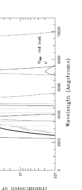
Figure 1:

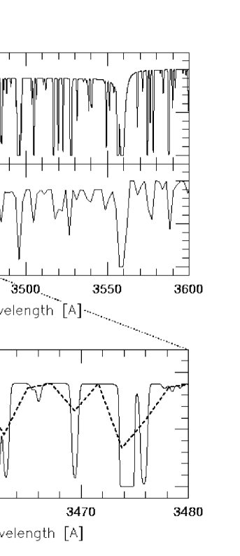
Figure 2:

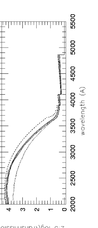
Figure 3:

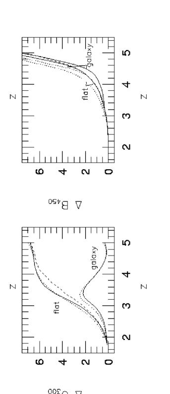
Figure 4:

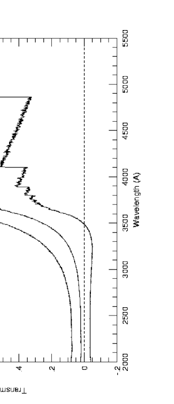
Figure 5:

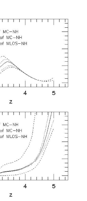
Figure 6:

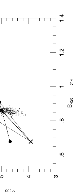
Figure 7: a

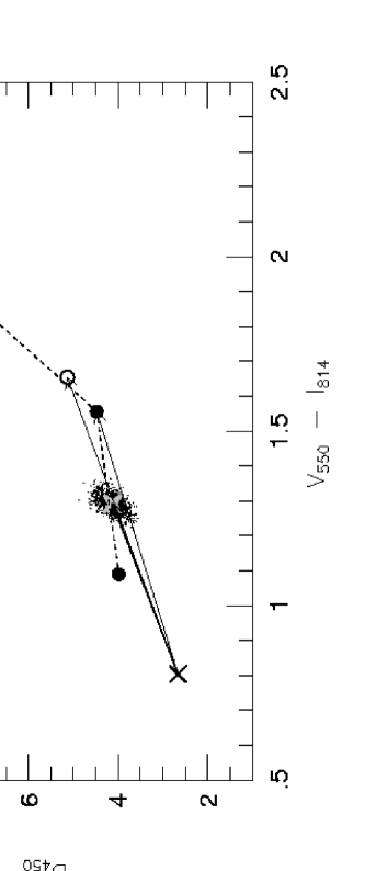
Figure 7: b

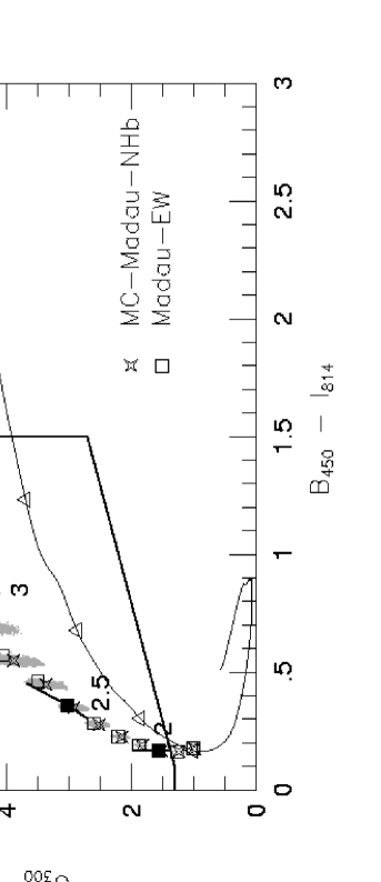
Figure 8: a

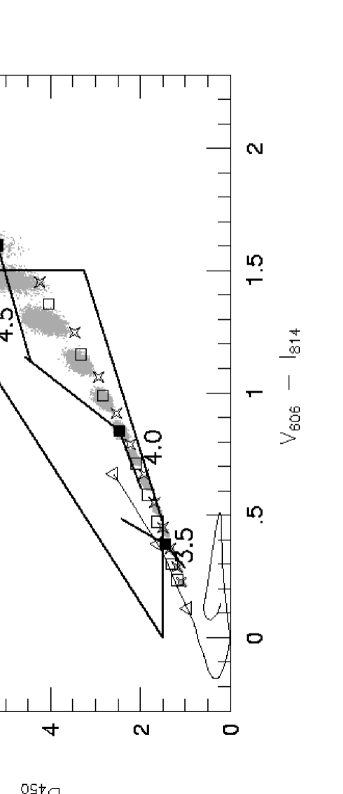
Figure 8: b

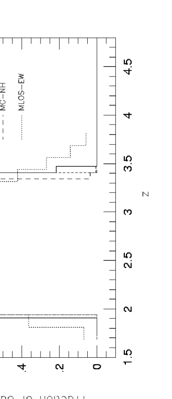
Figure 9: a

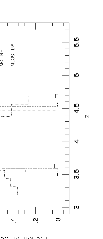
Figure 9: b

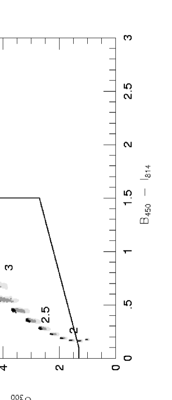
Figure 10: a

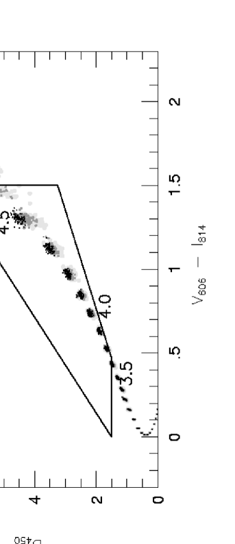
Figure 10: b

References

- (1)
- (2) Bruzual, A. G. & Charlot, S. 1993, ApJ, 405, 538
- (3)
- (4) Calzetti, D. 1997, in “The Ultraviolet Universe at Low and High Redshift”, ed. W. Waller, (Woodbury: AIP Press), astro-ph/9706121
- (5)
- (6) Davis, M., Wilkinson, D. T. 1974, ApJ, 192, 251
- (7)
- (8) Deharveng, J.-M., Faisse, S., Milliard, B., Le Brun, V. 1997, A&A, 325, 1259
- (9)
- (10) Dickinson, M. 1998, to appear in “The Hubble Deep Field,” eds. M. Livio, S.M. Fall, P. Madau, astro-ph/9802064
- (11)
- (12) Dove, J. B., Shull, J. M. 1994, ApJ, 423, 196
- (13)
- (14) Fall, S. M., Pei, Y. C. 1993, ApJ, 402, 479
- (15)
- (16) Ferguson, A. M. N., Wyse, R. F. G., Gallagher, J. S. 1996, AJ, 112, 2567
- (17)
- (18) Giallongo, E., Trevese, D. 1990, ApJ, 353, 24
- (19)
- (20) Guhathakurta, P., Tyson, J. A., Majewski, S. R. 1990, ApJ, 357, L9
- (21)
- (22) Heisler, J., Ostriker, J. P. 1988, ApJ, 332, 543
- (23)
- (24) Kim, T.-S., Hu, E. M., Cowie, L. L., Songaila, A. 1997, AJ, 114, 1
- (25)
- (26) Koo, D. C. 1981, Ph.D. thesis, Berkeley
- (27)
- (28) Koo, D. C. 1986, in “The Spectral Evolution of Galaxies,” eds. C. Chiosi and A. Renzini (Dordrecht, Reidel), 419
- (29)
- (30) Koo, D. C., Kron, R. G. 1980, PASP, 92, 537
- (31)
- (32) Leitherer C., Ferguson, H. C., Heckman, T. M., Lowenthal, J. D. 1995, ApJ, 454, L19
- (33)
- (34) Lockman, F. J., Jahoda, K., McCammon, D. 1986, ApJ, 302, 432
- (35)
- (36) Lowenthal, J. D. et al. 1997, ApJ, 481, 673
- (37)
- (38) Madau, P. 1995, ApJ, 441, 18
- (39)
- (40) Madau, P., Ferguson, H. C., Dickinson, M., Giavalisco, M., Steidel, C. C., Fruchter, A. 1996, MNRAS, 283, 1388
- (41)
- (42) Majewski, S. R. 1988, in “Towards Understanding Galaxies at Large Redshift,” eds. R. G. Kron and A. Renzini, (Dordrecht, Kluwer), 203
- (43)
- (44) Meier, D. L. 1976, ApJ, 207, 343
- (45)
- (46) Partridge, R. B. 1974, 192, 241
- (47)
- (48) Patel, K., Wilson C. D. 1995a, ApJ, 451, 607
- (49)
- (50) Patel, K., Wilson C. D. 1995b, ApJ, 453, 162
- (51)
- (52) Pettini, M. Steidel, C. C., Dickinson, M., Kellogg, M., Giavalisco, M., Adelberger, K. L. 1997, in “The Ultraviolet Universe at Low and High Redshift”, ed. W. Waller, (Woodbury: AIP Press), astro-ph/9707200
- (53)
- (54) Reimers, D. et al. 1992, Nature, 360, 561
- (55)
- (56) Rudloff, K., and Baggett, S. 1995, anonymous ftp archive
- (57)
- (58) Steidel, C. C. & Hamilton, D. 1993, AJ, 105, 2017
- (59)
- (60) Steidel, C. C., Pettini, M. & Hamilton, D. 1995, AJ, 110, 2519 (S95)
- (61)
- (62) Steidel, C. C., Giavalisco, M., Pettini, M., Dickinson, M., & Adelberger, K. L. 1996, ApJ, 462, L17 (S96)
- (63)
- (64) Steidel, C. C., Adelberger, K. L., Dickinson, M., Giavalisco, M., Pettini, M., Kellogg, M. 1998, ApJ, 293, 428
- (65)
- (66) Vogt, S. S. et al. , 1994, SPIE, 2198, 362
- (67)